Membangun Peta Bahaya Banjir Rob di Wilayah Pesisir (Studi Kasus: Surabaya, Jawa Timur, Indonesia).

(1)

ESTABLISHING HAZARD MAP

FOR TIDAL FLOOD IN COASTAL REGION

CASE STUDY: SURABAYA, EAST JAVA, INDONESIA

A B D U L W A H I D M U K L I S

GRADUATE SCHOOL

BOGOR AGRICULTURAL UNIVERSITY BOGOR

(2)

STATEMENT

I, Abdul Wahid Muklis states that thesis entitled:

ESTABLISHING HAZARD MAP FOR TIDAL FLOOD IN COASTAL REGION

CASE STUDY: SURABAYA, EAST JAVA, INDONESIA

is result of my own work under supervision of supervisory committee during the period April 2010 – June 2011 and it has not been published. The content of this thesis has been examined by the advising committee and an external examiner.

Bogor, July 2011

(3)

ABSTRACT

ABDUL WAHID MUKLIS. Establishing Hazard Map for Tidal Flood in Coastal Region (Case Study: Surabaya, East Java, Indonesia).

Under the direction of I NENGAH SURATI JAYA and IBNU SOFIAN.

This study examined the use of MRI-CGCM (Meteorological Research Institute- Coupled Atmosphere Ocean General Circulation Model) to predict sea level rise from 2010 to 2100. The DEM SRTM 30 m spatial resolution and sea level rise prediction were used to determine the level of inundation classes. In 2010 the prediction of sea level rise is about 2.1 m high and inundated about 1048 hectare of Surabaya area, causing total loss amounted to 370 billion rupiahs. The study also shows that the sea level at 2100 will rise around 2 m higher than occurred in 2010. The ground verification survey shows that there is a good prediction of sea level rise in 2010, where the predicted sea level rise is about 2.13 m while the actual rise is 2 m. The study concludes that the MRI-CGCM model was quite good to predict sea level rise having accuracy of 93.3%.

(4)

ABSTRAK

ABDUL WAHID MUKLIS. Membangun Peta Bahaya Banjir Rob di Wilayah Pesisir (Studi Kasus: Surabaya, Jawa Timur, Indonesia).

Dibawah bimbingan I NENGAH SURATI JAYA dan IBNU SOFIAN.

Penelitian ini mengkaji penggunaan MRI-CGCM (Meteorology Research Institute - Coupled Atmosphere Ocean General Circulation Model) untuk memprediksi kenaikan air laut dari tahun 2010 sampai dengan 2100. DEM SRTM dengan resolusi spasial 30 m dan hasil prediksi kenaikan air laut digunakan untuk menentukan kelas genangan. Pada tahun 2010, diprediksi kenaikan permukaan laut sekitar 2,1 m dan akan menggenangi areal seluas 1.048 hektar, dengan perkiraan total kerugian sebesar 370 miliar rupiah. Hasil penelitian menunjukkan bahwa permukaan laut pada 2100 diperkirakan akan meningkat sekitar 2 m lebih tinggi dari 2010. Hasil verifikasi di lapang menunjukkan bahwa diperoleh tingkat prediksi yang cukup baik untuk tahun 2010, dimana prediksi kenaikan permukaan air laut berdasarkan model adalah sekitar 2,13m, sementara kenaikan sesungguhnya adalah 2 m. Penelitian menyimpulkan bahwa model MRI-CGCM cukup baik untuk memprediksi kenaikan permukaan air laut, dengan tingkat akurasi sebesar 93,3%.

(5)

S U M M A R Y

ABDUL WAHID MUKLIS. Establishing Hazard Map for Tidal Flood in Coastal Region (Case Study: Surabaya, East Java, Indonesia).

Under the direction of I NENGAH SURATI JAYA and IBNU SOFIAN.

Several studies and observations have proven that the sea level is rising globally. Since 1990 sea level has been rising at 3.4 millimetres per year, twice as fast as on average over the 20th century. The researchers predicted the global sea levels will rise exceed to 200 cm in the 21st century (Vermeer, 2009; Grinsted et al., 2009; and Jevrejeva et al., 2010). Rising of sea level has an impact that includes: decimate the national territory, decreases coral reef populations, sinking islands, economic loss, etc. The sea level has not risen uniformly from region to region, as well as the impact of sea level rise is also diverse among coastal regions. The impact depends on each characteristic of the regional coastal which is influenced by interaction between lithology, geomorphology, wave climate condition, currents and storm frequencies.

As a part of East Java province, Surabaya city is located on coastal region, which located at 112°36’-112°21’ East and 7°12’-7°21’ South. The extent of Surabaya city area is 34,465 ha, consisting of 31 sub-districts with 163 villages. Historically, the lowland of Surabaya city came from the sediment formation of the sea area. Surabaya city has high potency in economic and infrastructure asset. Surabaya city has PDRB (Domestic Bruto Regional Product in million) is about 154 billion rupiahs and population is about 3 million (BPS, 2009). The tidal flood frequently occurs in Northern and Eastern part of Surabaya city, where located nearby the coastal.

This research was focused on the prediction of sea level rise in common and extreme condition on the basis of MRI-CGCM data model, as well as establishment vulnerability affected by tidal flood in coastal region of Surabaya city. The main objective of this research is to establish a hazard map on the basis of the prediction inundation area in 2010, 2030 and 2100, where the 2010 was threated as reference year. The loss estimation also developed for 2010, 2030 and 2100.

The applied methodology comprises four phases, namely; (1) Preparation and data acquisition: literatures review, primary data collection, and problem identification. (2) Pre-processing: development of vulnerable map as a reference to determine feasible area at the fieldwork phase. (3) Fieldwork: observation and measurement of inundation, and interviewed with local residents; (4) Processing and reporting: processing data, analysis data and reporting.

(6)

Loss estimation involves the calculation of the vulnerable area with the landuse cost damage. The estimation is only limited to the tangible damage or physical direct damage caused by tidal flood. Hypothetical prices of the landuse types were assigned based on previous of hazards flood report and on personal experience of the author in field survey. The predominant vulnerable landuse areas are residential, building and embankment. The embankment zone is divided into fish and salt pond.

The research results shows that the values of sea level projection on common condition in 2010, 2030 and 2100 are 2.13 m, 2.54 m and 4.13 m respectively; while the value of sea level projection on extreme condition in 2010, 2030 and 2100 are 2.93 m, 3.34 m and 4.93 m respectively. The estimated total loss are about 370 billion rupiahs, 2 trillion rupiahs and 3,6 trillion rupiahs for 2010, 2030 and 2100 respectively. On the basis of ground survey performed in 2010, the actual inundation in 2010 is ranging from 0.3 m to 0.35 m in area with elevation 1.7 m and about 0.6 m asl within area with elevation 1.4 m asl. The prediction derived from the model provides a good performance having 93% accuracy level.

(7)

1. It is prohibited to cite all of part of this thesis without referring to and mentioning the sources;

a. Citation only permitted for the sake of education, research, scientific writing, report writing, critical writing or reviewing scientific problem.

b. Citation does not inflict the name and honor of Bogor Agricultural University.

(8)

ESTABLISHING HAZARD MAP

FOR TIDAL FLOOD IN COASTAL REGION

CASE STUDY: SURABAYA, EAST JAVA, INDONESIA

A B D U L W A H I D M U K L I S

A thesis submitted for the degree Master of Science in Information Technology for Natural Resources Management Program Study

GRADUATE SCHOOL

BOGOR AGRICULTURAL UNIVERSITY BOGOR

(9)

Research Title : Establishing Hazard Map for Tidal Flood in Coastal Region Case Study: Surabaya, East Java, Indonesia

Name : Abdul Wahid Muklis Student ID : G 051060111

Study Program : Master of Science in Information Technology for Natural Resource Management

Approved by, Advisory Board

Prof. Dr. I Nengah Surati Jaya, M.Agr. Supervisor

Dr. Ibnu Sofian, M.Eng. Co-Supervisor

Endorsed by,

Program Coordinator

Dr. Ir. Hartrisari Hardjomidjojo, DEA

Dean of Graduate School

Dr. Ir. Dahrul Syah, M.Agr.Sc.

Date of Examination: Date of Graduation:

(10)

ACKNOWLEDGEMENTS

Alhamdulillahi Robbil ‘Alamiin, Praise be to ALLOH SWT Lord of the

Worlds, The Entirely Merciful, The Especially Merciful. Finally I could finish

my thesis.

Firstly, I would like to express my gratitude to my supervisors: Prof. I

Nengah Surati Jaya and Dr. Ibnu Sofian, for their assistance, encouragement

and patience, for guiding me in completing my thesis. My gratitude also goes

to Dr. Hartrisari, the Msc in IT for NRM program coordinator, Dr. Antonius

B.W. as the external examiner as well as thanks to all staff in MIT-Biotrop.

Sincerely thank is also extended to Mr. Leksono Wibowo, for the

survey guidance. Many thanks are also delivered to all my colleagues, friends

and all MIT students, there are too numerous to thank individually. Thank’s

guys.

To my lovely mom, dad, brother, cousin, auntie, uncle and all of my

family, thank you for always support, and being there for me, especially

during my difficult time.

"My Lord, enable me to be grateful for Your favor which You have

bestowed upon me and upon my parents and to work righteousness of which

You will approve and make righteous for me my offspring. Indeed, I have

repented to You, and indeed, I am of the Muslims." (QS 46:15)

(11)

CURRICULUM VITAE

The author was born on January 20th 1980 in Malang, East Java. In 1989 he and his family moved to Jakarta, and until now lived in Bekasi, West Java. In September 1999 he enrolled in the Plant Breeding study program, Agriculture Faculty of Brawijaya University, and graduated in June 2005 with the Final research title “Yield potential test and Resistance of yardlong bean (Vigna sesquipedalis) lines towards CABMV (Cowpea Aphid Borne Mosaic Virus).” The fund of his final research is obtained from Competence Grants Dikti (General Director of Indonesian College). In October 2006, the author registered in the graduate school at Master of Science in Information Technology for Natural Resources & Management program, Bogor Agricultural University (IPB). His M.sc. thesis entitled “Establishing Hazard Map for Tidal Flood in Coastal Region, Case Study: Surabaya, East Java, Indonesia.” He also worked freelance for projects, active in logo design competition, and also as internet marketer. The awards which has obtained are 1st rank world logo design contest of Mandy’s jewelry logo and 2nd rank of Raul Leal Incorporated, Alamako Incorporated International, 3rd rank Best Radar Detector logo in logomyway.com.

(12)

T A B L E O F C O N T E N T S

Abstract ……….. Summary ……… Acknowledgements ……… Table of content ……….. List of figures ………. List of tables ………...

Page

ii iv viii

x xii xiii

I. INTRODUCTION ... 1

1.1. Background ... 1

1.2. Objective of Research ... 2

1.3 Research Output ... 2

II. LITERATURE REVIEW ... 3

2.1 Sea Level Rise ... 3

2.2 Sea Level Projection According IPCC Model ... 7

2.3 MRI-CGCM in SRES A1B Model ... 10

2.4 Land Subsidence ... 11

2.5 El Niño and La Nina ... 12

2.6 Tidal Wave ... 15

2.6.1 Mean Sea Level by Moon and Sun Gravity ... 16

2.7 Addressing Tidal Flood Hazard ... 17

III. METHODOLOGY AND MATERIALS ... 19

3.1 Study Site ... 19

3.2 Data ... 20

3.3 Required Tools ... 21

3.4 General Method ... 22

3.4.1 Preparation and data acquisition ... 24

3.4.2 Pre-processing ... 24

3.4.3 Fieldwork ... 25

3.4.4 Processing and Reporting Phase ... 28

(13)

3.5.1 MRI data Model ... 31

3.5.2 Average High Wave Data ... 31

3.5.3 Maximum High Wave Data ... 31

3.5.4 Average between Maximum and Minimum Tides ... 31

3.5.5 Subsidence level estimation ... 32

3.5.6 High wave in El Nino and La Nina ... 32

IV. RESULT AND DISCUSSION ... 33

4.1 Sea Level Prediction ... 33

4.1.1 Sea Level Prediction for 2010 ... 33

4.1.2 Flood Prediction for 2010 ... 33

4.2 Loss Estimation ... 40

V. CONCLUSIONS AND RECOMMENDATION ... 42

5.1 Conclusions ... 42

5.2 Recommendations ... 42

REFERENCES ... 43

(14)

L I S T O F F I G U R E S

Page

Figure 2.1: Global of Mean Sea Level source from White (2009) ... 3

Figure 2.2: Causes of sea level rise from climate change ... 4

Source from Griggs (2001) ... 4

Figure 2.3: Global average sea level rise 1990 to 2100 by several of the SRES scenarios source from: IPCC (2001) ... 10

Figure 2.4: El Niño Condition source: NOAA (2010) ... 12

Figure 2.5: Normal Conditions source: NOAA (2010) ... 13

Figure 2.6: La Nina Condition source: NOAA (2010) ... 14

Figure 2.7: Niño3.4 Sea Surface Temperature Anomaly source: OOPC (2010) ... 14

Figure 2.8: a) Sea Level Related to Earth Gravitation, b) Gravity Anomalysource from: Fraczek (2003) ... 15

Figure 2.9: a) Forces Gravity Formation Evoke Spring Tide, b) Forces Gravity Formation Evoke Neap Tide ... 16

Figure 2.10: Tidal Level Patterns ... 17

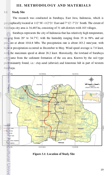
Figure 3.1: Location of Study Site ... 19

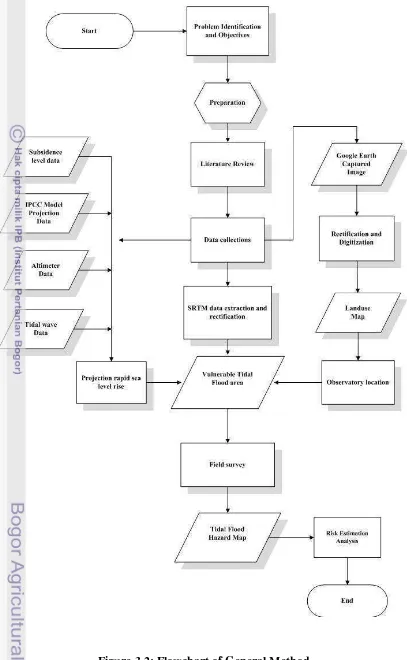
Figure 3.2: Flowchart of General Method ... 23

Figure 3.3: Efforts to Reduce Flood Impact ... 26

Figure 3.4: Surveyed Area of Tidal Flood Condition ... 27

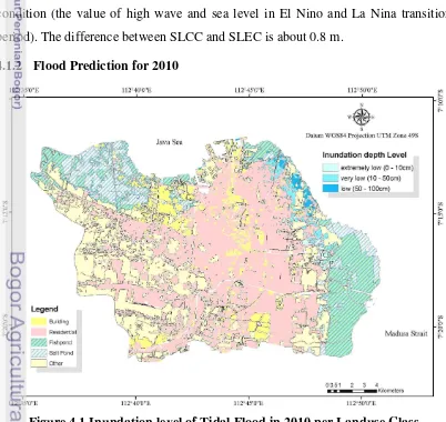
Figure 4.1 Inundation level of Tidal Flood in 2010 per Landuse Class ... 33

Figure 4.2 Graph of Tidal Flood in 2010 Area per Inundation Level ... 34

Figure 4.3 Field Survey in Pabean Cantikan sub-District ... 35

Figure 4.5 Graph of Tidal Flood in 2030 Area per Inundation Level ... 37

Figure 4.7: Graph of Tidal Flood in 2100 Area per Inundation Level ... 39

(15)

L I S T O F T A B L E

Page

Table 2.1: Sinking Island and Vulnerable Area Caused by Sea Level Rise ... 6

Table 2.2: The four of SRES scenario families ... 8

Table 2.3: Temperature and sea level rise for each SRES scenario family ... 9

Table 3.1: Vulnerability values for different landuse categories, in relation to four different water depth inundation level intervals ... 29

Table 4.1: Prediction total flood area 2010 in three inundation level ... 34

Table 4.4: Loss estimation of landuse type in relation to the inundation intervals ... 40

Table 4.5: Estimation loss of landuse type related with inundation level in 2010 .... 40

Table 4.6: Estimation loss of landuse type related with inundation level in 2030 .... 40

(16)

I . I N T R O D U C T I O N

1.1. Background

The global warming as a consequence of rapid growth of population and industrialization (anthropogenic forcing), has impact to the global climate and the environment. One of the impacts of global warming is sea level rise. Sea level rise related to the changes in global temperature which become warmer. There are some main processes influencing for sea level rise, namely: thermal expansion, ocean current variations, submarine topography, the melting of glaciers and ice caps, and the loss of ice from the Greenland and West Antarctic ice sheets (Douglas et al., 2000; IPCC, 2007; Kinver, 2008).

Since 1990 sea level has been rising at a rate of 3.4 millimetres per year, twice as fast as its average over the 20th century. Those conditions were linked the rate of sea level by global temperature rise. The temperature is getting warmer causing faster sea level rises. There is a correlation between global sea level and global temperatures. According to recent report by the Intergovernmental Panel on Climate Change (IPCC) estimates that in response to rising temperatures (1.0°-3.5°C) higher than 1990 levels in 2100), sea level will have risen by around 15-95 cm by the year 2100. Having correlated temperature history with sea-level history, Rahmstorf (2007) estimated future sea level position based on projections of future temperature.

The researchers predicted the global sea levels will rise exceed to 200 cm in the 21st century (Vermeer, 2009; Grinsted et al., 2009; and Jevrejeva et al., 2010). Rising of sea level has an impact including: decimating the national territory, decreasing coral reef populations, sinking islands, economic loss, etc.

(17)

One form of the sea level rise impact is tidal flood. Tidal flood may occur due to high tide wave overflowing coastal land. Today about 50% of the world's population lives in this critical interface between land and water, where 13 of the world's 20 largest cities are located at the coastal regions. Cohen et al (1997) estimated that in 1994 about 2.1 billion people (37% of the world's population) lived within 100 km of a coast. However increasing populations and development of the largest cities are placing significant stresses on the losses and other resources destruction, when the disaster caused by the rise of sea level appeared.

In Indonesia, tidal flood occurred almost on all of Northern region of the Java Islands (Pantura), such as Jakarta, Subang, Cirebon, Semarang, and Surabaya. Sofian (2008) reported that rapid sea level rise in Jakarta, Semarang, and Surabaya, predicted causing the inundation (flood) in area having elevation between 0 and 4 meter above sea level. Moreover the dynamic (climate anomaly) of the climate hazards could also raise the amount of the tidal flood.

Surabaya as the second largest Indonesian city has more valuable to the study; it is driven by the economic rationalities with PDRB (Domestic Bruto Regional Product in million) about 154 billion rupiahs and population about 3 million (BPS, 2009). Tidal flood may cause diseases, economical loss and also damage to the infrastructure (corrosive). Wuryanti (2002) said there is an indication of the sea level rise in Surabaya; the tidal flood for 12 ~ 48 hours in 2002 had caused inundation level in range between 5 to 100 cm. In last January and 19th February 2010 there was tidal flood in some area of Surabaya with inundation level ranging from 20 to 160 cm within 30 minutes to 6 hours (Iwa, 2010).

This research is study about the prediction of the sea level rise in common and extreme conditions on the basis of MRI-CGCM data model, and examining vulnerable area which affected by tidal flood in coastal region of Surabaya city.

1.2. Objective of Research

The objective of this research is to establish a hazard map on the basis of the prediction inundation area in 2030 and 2100; in which 2010 data were used as reference year.

1.3 Research Output

(18)

I I . L I T E R A T U R E R E V I E W

2.1 Sea Level Rise

There are a lot of observations shows that the sea level has been rising over the past several decades. The recent report of the Intergovernmental Panel on Climate Change (IPCC) estimates that in response to rising temperatures (1.0°-3.5°C higher than 1990 levels in 2100), sea level will have risen from 15 to 95 cm by the year 2100. Moreover global sea level could rise: between 75 to 190 cm (Vermeer, 2009). Nunn (2001) noticed, since the 1800’s, sea level in the Pacific has been rising then in the last century this rise has been recorded at about 15 cm and it is predicted that this rise will be at least twofold in the next century, meanwhile the projected sea level rise in Java Sea Indonesia is ranging from 60 to 78 cm until year 2100 (Sofian, 2008).

Figure 2.1: Global of Mean Sea Level source from White (2009)

(19)

A new scientific study warns that sea level could rise faster than previously projected. Since 1990 sea level has been rising at 3.4 millimetres per year, twice as fast as on average over the 20th century. Those condition were linked affected the rate of sea level by global temperature rise. The temperature is getting warmer causing faster sea level rises.

Many experts declared that global warming is the main factor that contributes to the sea level rise. Thermal expansions which come from greenhouse gases as trap heat energy in the atmosphere, transferred to the ocean and it may increasing the ocean volume. As impact of global warming, the rising temperature may cause mountain glaciers and ice sheets to melt and then sending the resulting melting water into the sea. Added by Gardiner et al (2004), effect of the global warming can cause ocean current variations which move vast quantities of water from one side of the southern Pacific to the other ocean area (El Nino).

Figure 2.2: Causes of sea level rise from climate change

(20)

A significant sea level rise is one of the major anticipated consequences of climate change. The Figure 2.2 explains the causes of sea level change according to the Intergovernmental Panel on Climate Change (IPCC). It explains the IPCC's A1 scenario family, which consists of three scenarios on future use of fossil energy sources, including scenario A1F1, which involves the use of fossil-intensive energy sources. This resource also includes the graphic 'Components of Mean Sea Level Rise for the Scenario A1F1' which shows the projected sea level rise in metres by 2050 and by 2100 for Greenland, glaciers, expansion, the Antarctic, and the total sea level rise (Griggs, 2001).

Rolalisasi (2008), divides the sea level rise impacts into; physical impact and socio economic impact. The physical impact includes inundation and displacement of lowlands and wetlands; coastal erosion intensification of storm flooding, increase in salinity of estuaries, salt-water intrusion into freshwater aquifers, and degradation of water quality, change of tide in rivers and bays, change of sediment deposition patterns. The socio-economic impact includes; the increased loss of property and fisherman settlements, increased flood risk and potential loss of life, damage to coastal protection works and other infrastructure.

Mcgranahan et al., (2007) noted that approximately 10% of the world’s population, or about 600 million people, are live in low land areas which vulnerable of being flooded. The sea level rise impact may cause change the border of the country due to the sinking of the outer islands which used as reference for ZEE (Economic Exclusive Zone). In Indonesia may cause reduction of inland area and more than 3000 islands will be sinking in future when the 25 meter of the shoreline is declined then will cause the lost of 202.500 Ha of coastal area by the end of 2100 (Diposaptono, 2002; Rais, 2007; Salim, 2008).

The following are the data of submerged islands due to sea level rise, according (SMT, 2010):

• Lohachara, India – 10,000 residents

• Bedford, Kabasgadi and Suparibhanga islands near India – 6,000 families • Chesapeake Bay in Maryland, USA – 13 islands

• Kiribati – 3 atolls

(21)

The following table, are recorded data of the sinking islands and or at risk from rising sea levels:

Table 2.1: Sinking Island and Vulnerable Area Caused by Sea Level Rise

Location Description

Tuvalu 12,000 residents with no more fresh drinking water and vegetable plots have washed away.

Ghoramara near India 2/3 submerged as of 2006 with 7,000 residents already relocated.

Neighboring island of Sagar 250,000 residents also threatened, some 50 other islands were jeopardized in the India-Bangladesh Sundarbans, with a population of 2 million.

Kutubdia in southeastern Lost over 200,000 residents Bangladesh 150,000 likely soon to depart.

Maldives 369,000 residents in the Indian Ocean, whose president wants to relocate the entire country.

Marshall Islands 60,000 residents.

Kiribati 107,800 residents, approximately 30 islands submerging.

Tonga 116,900 residents.

Vanuatu 212,000 residents, some of whom have already been evacuated and coastal villages relocated.

Solomon Islands 566,800 residents. Carteret Islands in Papua

New Guinea

2,500 residents whose land no longer supports agriculture.

Shishmaref in Alaska, USA 600 residents. Kivalini in Alaska, USA 400 residents.

Indonesia Over 2,000 islands sink.

Dubai 1.2 million residents in the United Arab Emirates considered at risk.

Source from: SMT (2010)

(22)

mostly due to non-uniform changes in temperature and salinity and related to changes in the ocean circulation. As-syakur (2007) noted, that Indonesia is belong to this condition where occurrence of main convergence of two main world circulation (walker and hardly). Location of Indonesia is between 2 continents and ocean so that has a circulation (monsoon) due to sun movement and of course the occurrence of ENSO (el-nino and la-nina). Variation of topographic in all region of Indonesia, (mountains, forests, valley, etc) causing variation of climate and sea level condition.

2.2 Sea Level Projection According IPCC Model

A set of scenarios was developed by Intergovernmental Panel on Climate Change (IPCC) to represent the range of driving forces and emissions in the scenario literature so as to reflect current understanding and knowledge about underlying uncertainties. Those scenarios assist in climate change analysis, including climate modelling and the assessment of impacts, adaptation, and mitigation.

The scenarios are based on an extensive assessment of driving forces and emissions in the scenario literature, alternative modelling approaches, and an “open process” that solicited wide participation and feedback. The open process defined in the Special Report on Emissions Scenarios (SRES) Terms of Reference calls for the use of multiple models, seeking inputs from a wide community as well as making scenario results widely available for comments and review. These objectives were fulfilled by the SRES multi-model approach and the open SRES website (IPCC, 2000).

(23)

Table 2.2: The four of SRES scenario families

AR4

(Fourth Assessment Report)

More economic focus More environmental focus

Globalisation (homogeneous world)

A1

rapid economic growth (groups: A1T; A1B;

A1Fl) 1.4 - 6.4 °C

B1

global environmental sustainability 1.1 - 2.9 °C

Regionalisation (heterogeneous world)

A2

regionally oriented economic development

2.0 - 5.4 °C

B2

local environmental sustainability 1.4 - 3.8 °C

Source from: IPCC (2001)

The A1 storyline and scenario family describes a future world of very rapid economic growth, and global population that peaks in mid-century and declines thereafter, as well as the rapid introduction of new and more efficient technologies. Major underlying themes are convergence among regions, capacity building, and increased cultural and social interactions, with a substantial reduction in regional differences in per capita income. The A1 scenario family develops into three groups that describe alternative directions of technological change in the energy system. The three A1 groups are distinguished by their technological emphasis: fossil intensive (A1FI), non-fossil energy sources (A1T), or a balance across all sources (A1B).12

The A2 storyline and scenario family describes a very heterogeneous world. The underlying theme is self-reliance and preservation of local identities. Fertility patterns across regions converge very slowly, which results in continuously increasing global population. Economic development is primarily regionally oriented and per capita economic growth and technological changes are more fragmented and slower than in other storylines.

(24)

The B2 storyline and scenario family describes a world in which the emphasis is on local solutions to economic, social, and environmental sustainability. It is a world with a continuously increasing global population at a rate lower than in A2, intermediate levels of economic development, and less rapid and more diverse technological change than in the B1 and A1 storylines. While the scenario is also oriented towards environmental protection and social equity, it focuses on local and regional levels (IPCC, 2001).

Table 2.3 shows about six families of SRES scenarios and AR4 (Fourth Assessment Report), provide projected temperature and sea level rises (excluding future rapid dynamical changes in ice flow) for each scenario family.

Table 2.3: Temperature and sea level rise for each SRES scenario family

Scenario (SRES) Description

1 B1 Best estimate temperature rise of 1.8 °C with a likely range of 1.1 to 2.9 °C. Sea level rise likely range 18 to 38 cm. 2 A1T Best estimate temperature rise of 2.4 °C with a likely range

of 1.4 to 3.8 °C. Sea level rise likely range 21 to 48 cm.

3 B2 Best estimate temperature rise of 2.4 °C with a likely range of 1.4 to 3.8 °C. Sea level rise likely range 20 to 43 cm

4 A1B Best estimate temperature rise of 2.8 °C with a likely range of 1.7 to 4.4 °C. Sea level rise likely range 21 to 48 cm.

5 A2 Best estimate temperature rise of 3.4 °C with a likely range of 2.0 to 5.4 °C. Sea level rise likely range 23 to 51 cm.

6 A1F1 Best estimate temperature rise of 4.0 °C with a likely range of 2.4 to 6.4 °C. Sea level rise likely range 26 to 59 cm.

Source from: IPCC (2000)

(25)

Figure 2.3: Global average sea level rise 1990 to 2100 by several of the SRES

scenarios source from: IPCC (2001)

A set of scenarios was developed to represent the range of driving forces and emissions in the scenario literature to reflect current understanding and knowledge about underlying uncertainties. The scenarios are based on an extensive assessment of driving forces and emissions in the scenario literature, alternative modelling approaches, and an “open process” that solicited wide participation and feedback.

Several data models projection with set of IPCC scenarios (SRES) has been done by some research institutes namely: BCC-CM 1 model (Beijing Climate Center, China), BCM 2.0 model (Bjerknes Centre for Climate Research, Norway), CGCM3.1 model (Canadian Centre for Climate Modelling and Analysis), MIROC3.2 (Model for Interdisciplinary Research on Climate, Japan), Mk3.0 & 3.5 model (CSIRO- Commonwealth Scientific and Industrial Research Organisation, Australia), HadCM3 model (Hadley Centre for Climate Prediction, UK), INMCM3.0 model (Institute for Numerical Mathematics, Russia), CM3 model from Meteo France, MRI model from Meteorogical Research Institute - Japan, GISS model (NASA-Goddard Institute for Space Studies), and CM 2.0 & 2.1 from NOAA, etc.

2.3 MRI-CGCM in SRES A1B Model

(26)

used in 1993. Data needed to develop this model is Global data of snow depth and density with several meteorological variables to drive, namely: precipitation, air temperature, wind speed, wind direction, humidity, down-welling long and short wave radiation, cloud cover, and surface pressure (Noda, 1999).

The SRES A1B was taken in this research, because the A1B scenario is being considered to represent the current trend of emissions IPCC data model projection used as reference and parameter to make projection in 2100 (Yamashiki et al., 2010). Takaya (2009) has reported that MRI-CGCM has high predictability of precipitation and air temperature over the Eastern Asia even without statistical applications. It is also noted that the seasonal prediction skills are strongly dependent on regions, seasons and the elements to predict as well as ENSO situations. Compared to AGCM (Atmospheric General Circulation Model), CGCM has improvement performance in forecast and high predictability response to the mid-latitude atmospheric circulation that appears behind an El Niño event (Naruse, 2009). Evaluation from Takaya (2008) noted that, this model has good performance in typhoon seasonal forecast, moreover Stockdale et al., (2009) added, within the fiscal 2009 year coupled model (JMA/MRI-CGCM) will be employed for all the JMA long-range forecasts.

2.4 Land Subsidence

Land subsidence is the lowering gradual process of the land-surface elevation that take place underground (Leake, 2004). These natural phenomena usually occur in big city within coastal area which standing on top of sediment layer such as Jakarta (Abidin et.al, 2009), Surabaya (Tobing, 2004), Semarang (Marfai, 2003), Bangkok (Phien-wej, et al., 2005), Osaka, Tokyo (Yamamoto, 1995), Shanghai (Wei, 2006), Taiwan (Chu and Sung, 2003), etc. There are some factors which cause land subsidence namely: excessive water suction, heavy building/ container (surface load force), intrusion, erosion, mud extraction (Lapindo case), oil and gas extraction, underground mining and tectonic movements.

(27)

2.5 El Niño and La Nina

El Niño and La Niña is an un-regularly weather phenomena which occur as the result from interaction between the surface of the ocean and the atmosphere in the tropical pacific. Changes in the ocean have impact to the atmosphere and climate patterns around the globe. In turn, changes in the atmosphere have impact to the ocean temperatures and currents. The system oscillates between warm (El Niño) to neutral (or cold La Niña) conditions with an on average every 3-4 years (NOAA, 1998).

El Niño is characterized by unusually warm of ocean temperatures in the Equatorial Pacific, as opposed to La Niña, which characterized by unusually cold ocean temperatures in the Equatorial Pacific. El Niño is an oscillation of the ocean-atmosphere system in the tropical Pacific having important consequences for global weather (NOAA, 2010).

Figure 2.4: El Niño Condition source: NOAA (2010)

As shown in Figure 2.4, the condition on western part of Pacific Ocean there is increasing of the air pressure, causing inhibition of cloud formation upon Eastern Indonesian sea, so that’s why in some region in Indonesia the rainfall was declined far from normal condition (also Figure 2.5), El Niño in Indonesia is usually related to drought condition. Gutman et al. (2000) said, that the El Niño made long dry period, declining of evaporation and precipitation, so that usually causing decreasing in food production.

(28)

middle of ocean pacific region. This condition uplift chlorophyll-a content and up-welling so that can increase the number of fish catches. Up-up-welling mean the transport movement of deeper water to shallow levels.

The year 2010 is anomalies for the climate in Indonesia because it affected by the extreme climate with is strong El-nino followed by strong LaNina (see appendix 1 and appendix 2). In July 2010, the extreme climate had caused displacement of large currents circulation (appendix 9), especially in the transition period between la-nina and el-nino, causing the sea levels rise. Meanwhile, December 2010 was in the strong LaNina phase sea level rise, with an additional mass of water in the sea of rain water (appendix 10) and also wind current from southwest of the Java islands (Indian Ocean region).

Figure 2.5: Normal Conditions source: NOAA (2010)

(29)

Figure 2.6: La Nina Condition source: NOAA (2010)

SOI (Southern Oscillation Index) used as indicator for describing El Nino and La Nina occurrences. The Southern Oscillation Index (SOI) is calculated from the monthly or seasonal fluctuations in the air pressure difference between Tahiti and Darwin (the western and Eastern tropical Pacific) during El Niño and La Niña episodes. The SOI graphics can be seen in appendices section. Positive values of the SOI are associated with stronger Pacific trade winds and warmer sea temperatures to the north of Australia, popularly known as a La Niña episode. While negative values refer to El Niño condition (NOAA, 2009).

Figure 2.7: Niño3.4 Sea Surface Temperature Anomaly source: OOPC (2010)

(30)

(Figure 2.7) the red colour is in El-nino condition while blue is La-Nina. The anomaly is calculated relative to a climatologically seasonal cycle based on the years 1982-2005 (OOPC, 2010). Nino3.4 zone condition is a reference to determine phase of El nino – La Nina because it is located in the middle of tropical Pacific zone and the movement of the currents started from here. The Oceanic Nino Index (ONI) from 1950 – 2010 can be seen in appendix 2; the ONI is calculated using Version 3b of the extended reconstructed sea surface temperature (ERSST) dataset. The extended reconstructed sea surface temperature (ERSST) was constructed using the most recently available International Comprehensive Ocean-Atmosphere Data Set (ICOADS) SST data and improved statistical methods that allow stable reconstruction using sparse data.

2.6 Tidal Wave

Tides are caused by gravity energy effects by moon and sun attraction. Periodically rise and fall of sea level cyclical influence of the Earth's rotation and also related to earth gravitation. There is difference tides energy in each coastal area, the energy of tides make a wave and impact to the level of the sea, those differences caused by different topographic surface layer in the sea, the shallow surface layer has higher sea level than a depth one (see Figure 2.8a). Other factor which influences the earth gravitation is the type of rock structure in the sea. In Figure 2.8b it is shown that the East part of Indonesia has higher than western (Indonesia ocean) in earth gravitation, so that the Eastern Indonesia has more high in sea level. The gradation green-yellow-orange color respectively means the low to high of gravitation level.

Figure 2.8: a) Sea Level Related to Earth Gravitation, b) Gravity Anomaly

(31)

2.6.1 Mean Sea Level by Moon and Sun Gravity

Sea level rate also influence by moon and sun gravity to earth, and the gravity forces in a year is constant as long as no changes in the position and material between moon and sun to the earth.

Figure 2.9: a) Forces Gravity Formation Evoke Spring Tide, b) Forces Gravity

Formation Evoke Neap Tide

Spring tides are usually strong tides (Figure 2.9a), when the formation of sun, moon and earth is in the line. These spring tides occur every 14-15 days during full and new moons. Meanwhile the neap tides (Figure 2.9b) occur when the gravitational forces of the Moon and the Sun are perpendicular to one another.

(32)

Figure 2.10: Tidal Level Patterns

2.7 Addressing Tidal Flood Hazard

The sea level rise and land subsidence is the main factors the occurrence of tidal flood hazard and it cause loss material. Tidal flood is one problem of coastal city as the impact of the climate hazard which is influenced by the sea level rise. In Pantura (Northern coastal of Java), Indonesia, the tidal flood occurred annually on almost all of region of the java coastal area, such as Jakarta, Subang, Cirebon, Semarang, and also Surabaya.

Surabaya is the city which is located in coastal area has the second densest population city in Indonesia, has importance economic rationalities. A consequence of the rapid migration and economic development in Surabaya is the high demand necessity of the clean water.

(33)

Surabaya city the rate of land subsidence is ranging from 0.02-0.25 m per year due to compressibility and also the sediment soil type.

(34)

I I I . M E T H O D O L O G Y A N D M A T E R I A L S

3.1 Study Site

The research was conducted in Surabaya, East Java, Indonesia, which is geographically located at 112°36’-112°21’ East and 7°12’-7°21’ South. The extent of Surabaya city area is 34,465 ha, consisting of 31 sub-districts with 163 villages.

Surabaya represents the city of Indonesia that has relatively high temperature, ranging from 20° to 34.7°C, with the humidity ranging from 35 to 98% and air pressure at about 1014.8 Mbs. The precipitation rate is about 183.2 mm/year, with highest precipitation occurred in December to May. Wind speed average is 7.0 knot, with the maximum speed at about 26.2 knot. Historically, the lowland of Surabaya city came from the sediment formation of the sea area. Known by the soil type predominantly found, i.e.: clay-sand (alluvial) and limestone hill in part of western Surabaya.

(35)

Surabaya municipal mostly belongs to lowland area with average altitude ranging from 3 to 9 meter above sea level. Meanwhile the hilly area is located in southwestern namely Bukit Lidah and Bukit Gayungan having altitude ranging from 25 to 50 meter.

The coastal areas span from the west municipal border to Tanjung Perak harbor and Eastern area of Sidoarjo regency border. The coastal area includes 9 sub-districts and 17 sub-districts. Generally the coastline is located in the Eastern and Northern as well as western part of the Surabaya city (Figure 3.2). In the Eastern part of Surabaya city, the predominant landuses are fish and salt ponds, wetland, fields, and swamp while in the Northern part is fish ponds, warehouse building, harbor with some settlement area.

3.2 Data

The main and supporting data used in this study include:

(a) IPCC data model for global sea level projection used from MRI – CGCM model with SRES A1B scenario. Data global sea level was derived from WCRP (World Climate Reseach Program) that can be accessed from https://esg.llnl.gov:8443/data.

(b) Tidal gauge data from University of Hawaii Sea level center and Indonesian Navy annual report (2010). The tidal data were derived from UHSLC (University of Hawaii Sea Level Center) which can be accessed in http://ilikai.soest.hawaii.edu/uhslc/datai.html. Data were provided from 1991 to 2004.

(c) SRTM (Shuttle Radar Topography Mission) acquired in 2006, with 30 m spatial resolution collected by National Mapping and Coordination Survey Agency (Bakosurtanal). SRTM/DEM data used for establish contour line and elevation model.

(36)

This data was used by author as a parameter to define maximum value of sea level in transition month of El-nino La-nina.

(e) RBI (Rupa Bumi Indonesia) Map 2001 at scale of 1:50.000 created by the National Mapping and Coordination Survey Agency (Bakosurtanal). The RBI map is topographic map in the form of digital vector data. The other data are landuse/ landcover map coupled with attribute data such as administration, river, road, etc. The RBI was used for mapping and tidal flood analysis.

(f) Surabaya subsidence level data for 2003 ~ 2004 which were derived from Indonesian Geology Bureau. The subsidence data was used as a parameter to calculate relative sea level.

(g) The Indonesian Navy tidal gauge annual report data were used as a reference and prediction of tidal floods occurrence can be done in Surabaya city.

(h) Interview data by the local resident and observation at the potential inundation areas.

3.3 Required Tools

To accomplish the study, the software and hardware used are as follows: (a) Software

1. Arc-Gis/view for GIS work and spatial analysis. 2. 3DEM for accessing and conversion of DEM.

3. WXTide 32 ver.4.7 for defining and measurement tides.

4. Panoply 2.9.4 for open the sea level dataset from AVISO and converted to preferable file format.

5. Google Earth ver. 4.2 is used for landuse delineation. (b) Hardware

1. PC Intel Core2 CPU T7200 2.00 GHz, 2 GB RAM, Mobile Intel 945GM Express Chipset Family.

(c) Tools

1. Global Positioning System (GPS) Garmin 76Csx for measuring geo-position in field work.

(37)

3. Printer HP 3420 for printing purpose.

3.4 General Method

(38)

(39)

3.4.1 Preparation and data acquisition

This phase consists of activities such as: literatures review, primary data collection, and problem identification. The literature studied deals with tidal flood, the climate hazard impact, sea level rise, el nino – la nina phenomenon, and IPCC sea level projection by MRI model. This phase includes journals and previous research results collection which are related with this research. The primary data was collected in this phase from National Mapping and Coordination Survey Agency (Bakosurtanal), Indonesian Geology Bureau (Badan Geologi).

3.4.2 Pre-processing

Pre-processing phase includes the process for producing vulnerable map as a reference to determine feasible area at the fieldwork phase. The pre-processing data started by cropping DEM-SRTM, rectification (projected to UTM WGS 49S zone coordinate system), and convertion into grid format using 3DEM software.

The geometric data were used to determine the inundation area using the sea level projection formula. Let say the sea level relative calculation resulted 4 meter, it means in area with 3 meter elevation above sea level, the inundation level will be 1 meter depth, and in elevation 4 meter or more there is no inundation or not affected.

The next step is to define the value of sea level relative, by extracting raw data of high wave from AVISO and tide gauge raw data from UHSLC using Panoply software. The data were converted those data into Ms Excel format. Then putted the subsidence level data which gotten from Indonesian Geology Bureau in Ms Excel. Global mean sea level from IPCC model projection which has already downloaded from https://esg.llnl.gov:8443/data/ were extracted to text format file using Panoply software and converted into ms excel file format. All data has processed and calculated in Ms Excel software.

The formula of sea level relative is modification of the Sofian (2008) sea level projection equation, as follow:

TEE=MSL+HEL+HW+HPS+SL (1)

(40)

Prediction of the sea level was done for 2010, 2030, and 2100. The 1900 used as a baseline year measurement; so that the value at 2.1 meter of 2010 for example, is the rising of the sea from 1900. The projection was divided into common and extreme conditions. Common condition is the sea level in general climate while extreme condition is the sea level in the extreme climate condition namely in the transition period of El Nino-La Nina. Thus prediction of sea level especially in year period of El Nino and La Nina, range in between common and extreme condition.

The formula of common condition ( SLCC_{( )}_t ) and extreme condition

(SLEC_{( )}_t ) of sea level projection can be seen as follows:

( ) MSLM HW TWL LS

SLCC_t = ₍_t₎ + + + (2)

( )t MSLM(t) HWex TWL LS HEL(t)

SLEC = + + + + (3)

Where:

) (t

MSLM : Global Mean Sea Level in (t) year observed data according IPCC model projection.

HW : Average of high wave data.

HWex : Maximum value of high wave data.

TWL : Average range between maximum and minimum of tides data.

LS : Land subsidence data.

) (t

HEL : Sea level in (t) El Nino and La Nina transition period.

To define level inundation, the value of HW has to multiply by 30%, because wave energy to push sea water up to the mainland is decrease about 30% due to hit the material which stand on the coastline area.

The value of sea level relatives has resulted and use as guidance to specify the level of inundation in year observation. Then in same time, the data resulted was overlaid with the topographic map (RBI map), to make a vulnerable map that possible to be displayed and geo-processed using Arc-view software.

3.4.3 Fieldwork

(41)

condition related to the research, to conduct interviewed to the local residents, and to record the occurrence of tidal flood throughout 2010. Tidal flood observation was based on the existing vulnerable hazard map which has been made. The condition of tidal flood in Surabaya can be seen in appendix 8.

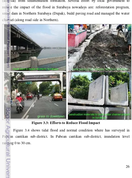
Flood impact might reduced by high sedimentation of Surabaya. According to the interview of local expert and survey, the sedimentation in Surabaya reaches 3 km per year. It was the fact that the predominant soil type of Surabaya is clay-sand (alluvial) from sedimentation formation. Several effort by local government to reduce the impact of the flood in Surabaya nowadays are: reforestation program, small dam in Northern Surabaya (Dupak), build paving road and managed the water channel (along road side in Northern).

Figure 3.3: Efforts to Reduce Flood Impact

(42)

Tidal Flood Normal

(43)

3.4.4 Processing and Reporting Phase

The reporting phase is finalizing phase of the research including discussion, i.e., writing, do some revision, consultation to the supervisor, co-supervisor and the expert, also all activity for thesis report accomplishment. This phase also describe about the risk prediction of losses which caused by floods.

According UN (2004), risk is defined as the probability of harmful consequences, or expected losses deaths, injuries, property, livelihoods, economic activity disrupted or environment damaged) resulting from interactions between natural or human-induced hazards and vulnerable conditions. Risk can be expressed as follows:

Risk = Hazard x Vulnerability. (3)

In this study the risk assessment is calculation of physical losses (tangible damage) from landuse types which was extracted from the Google Earth image. The risk assessment considered by vulnerable map that is resulted from previous phase (pre-processing). In this research, the risk estimation is only limited to the tangible damage or physical direct damage caused by tidal flood.

The method of risk damage calculation is:

V

H

R

=

Σ

*

(4)

Where:R= Risk damage (currency unit per unit area), ΣH = total cost damage (per unit area), and V = Vulnerability value. (UN, 2004)

Hypothetical prices of the landuse types were assigned based on previous of hazards flood report and on personal experience of the author in field survey. In this research, land use was divided into four classes because majority land use in Northern and Eastern Surabaya where located in range 0 ~ 6 km to the coastline are dominated by embankment zone (fish and salt ponds), residential, and warehouse building. So that only those four landuse type will be classified and calculated.

(44)

Table 3.1 presents the vulnerability values in relation to four different water depth inundation level intervals: <10 cm, 10–50 cm, 50–100 cm and 100–150 cm from Coto (2002). Meanwhile the embankment vulnerable value was derived from author assumed according survey.

Table 3.1: Vulnerability values for different landuse categories, in relation to

four different water depth inundation level intervals

Landuse type

Vulnerability values

<10 cm 10-50 cm 50-100 cm 100-150 cm Extremely Low Very Low Low Moderate

Residential 0.01 0.15 0.5 0.8

Warehouse Building 0 0.2 0.4 0.5

Embankment 0 0.25 0.5 1

Commercial 0.1 0.4 0.6 0.8

Agricultural field 0 0.05 0.1 0.2

Farm 0.01 0.1 0.2 0.25

Farm for crop 0.3 0.45 0.5 0.55

Source from Coto (2002)

The water depth inundation level in 2010, 2030 and 2100 were classified into: a. Extremely low; areas with inundation level from 0 to 10 cm.

b. Very low; areas with inundation level from 10 to 50 cm. c. Low; areas with inundation level from 50 to 100 cm. d. Moderate; areas with inundation level from 100 to 150 cm. e. High; areas with inundation level from 150 to 250 cm.

f. Very high; areas with inundation level from 250 to 400 cm and g. Extremely high areas with inundation level >400 cm.

The classifications of inundation level were established from the combination class inundation level created by Coto (2000) and the predicted sea level in 2010 to 2100. The classified value expected could comprise the inundation level within 2010 to 2100. Compared with sea level in 2100 where predicted rise up to 400 cm, the sea level rise prediction in 2010 (0 to 50 cm) in categorized into low level.

(45)

In residential area the cost value of heavy damage is 20 million rupiahs per unit, while light damage in residential area is about 5 million rupiahs per unit, and warehouse building is about 200 million rupiahs per unit (Bappenas, 2007). According to survey, usually the resident builds a dike after occurrence of the floods in the inundation of 10 cm depth, and it is reference to the low vulnerable value for residential. Total costs to build dikes per house approximately achieve 200 thousand rupiahs. The embankment is dividing into fish and salt, where for in fish/shrimp embankment the harvest price, is about 4.5 million per hectare per farming season (6 months) (Bappenas, 2000). Meanwhile in salt embankment, the harvest price is about 300 thousand rupiahs per hectare per farming at every 3 days (Purbani, 2003).

The detail of conversion amount of unit of each landuse type in one hectare can be illustrated as follows:

a. Residential area; the assumption per hectare of residential area are filled by 100 houses. Every house has size about 60 square meters so that for housing complex fill in area about 6000 square meter, and the rest area about 4000 square meter is using for terrace and collector road.

b. Warehouse; the warehouse criteria in this study is defined as more than one-story building which has an area exceeding 500 square meters and is used as commercial properties. The assumption of general building size is 500 square meter for each building and the rest about 5000 square meter for collector road and parking area, so that in one hectare will be consist of 10 buildings.

(46)

3.5 Sea Level Projection Component

3.5.1 MRI data Model

In order to obtain the sea level rise, the available model data in certain year was reduced by data in 1900, which were used as the baseline year when the first measurement of tidal gauge. Appendix shows that the value of sea level rise in 2010 (MSLM₂₀₁₀ ) is about 0.292 m, in 2030 (MSLM₂₀₃₀ ) is 0.287 m and in 2100 (MSLM₂₁₀₀) is 0.406 m.

3.5.2 Average High Wave Data

High wave data were obtained from University of Hawaii Sea Level Center (UHSLC), the complete data can be seen in Appendix 7. Calculation for defining inundation, the average value of high wave data has been multiplied by 30% due to hit to the material which stand on the coastline area.

HW = 1.054*30%

= 0.316 m.

3.5.3 Maximum High Wave Data

The maximum of high wave data was obtained from the highest or maximum value of high wave data and also multiplied by 30% due to hit to the material which stands on the coastline area.

HWex= 2.38*30% = 0.715 m.

3.5.4 Average between Maximum and Minimum Tides

The tide pattern was stated (see chapter 2.7.1) where there has a maximum and a minimum value from average data in any day. To predict the sea level, the distance value between maximum and minimum value has been measured. The tide data in this research were derived from WX Tide Software.

(47)

3.5.5 Subsidence level estimation

Subsidence’s in Surabaya is predicted and caused by the pressure of the heavy material such as building and heavy vehicles especially in Northern Surabaya which filled up by warehouse and freight transportation.

Subsidence level data have been obtained from Badan Geology with 2003 – 2004 data observation. For this research these subsidence level data used as reference to predict land subsidence year by year.

Subsidence value (SL(t)) is defined as the average of subsidence level data in

a year with an assumption that the value of subsidence level is similar to 2003-2004.

The average of subsidence level data

( )

SL can be calculated as follows,

1

t t=

∆ (year projected) −t₀ (year of available data), and the subsidence level

formulated as follow:

SL t

SL(t) =∆ * (6)

So that the value subsidence level in 2010, 2030 and 2100 is: 21

. 0 * ) 2004 2010

(

2010 = −

SL

= 0.12 m

21 . 0 * ) 2004 2030

(

2030 = −

SL

= 0.54 m.

21 . 0 * ) 2004 2100

(

2100 = −

SL

= 2.01 m.

3.5.6 High wave in El Nino and La Nina

(48)

I V . R E S U L T A N D D I S C U S S I O N

4.1 Sea Level Prediction

4.1.1 Sea Level Prediction for 2010

The projection sea level of common climate condition (SLCC) in 2010 is:

(2010)

SLCC = 0.292 m + 0.316 m + 1.40 m + 0.125 m

= 2.13 m.

The projection sea level of extreme climate (SLEC) in 2010 is:

(2010)

SLEC = 0.292 m + 0.714 m + 1.40 m + 0.125 m + 0.40 m

= 2.93 m.

According prediction sea level in 2010, the prediction inundation level occurred was an impact of sea level in a range from 2.13 m until 2.93 m. The difference of the result between SLCC and SLEC, were influenced by climate condition (the value of high wave and sea level in El Nino and La Nina transition period). The difference between SLCC and SLEC is about 0.8 m.

4.1.2 Flood Prediction for 2010

(49)

0 100 200 300 400 500 600

0-10 10-50 50-100

Extremely Low Very Low Low

Inundation level (cm)

H

e

c

ta

r

e

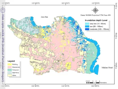
Figure 4.1 shows prediction inundation of common condition in 2010, based on calculation of SLCC (Sea Level in Common Condition), which has been classified into 3 inundation depth levels namely extremely low (0~10 cm), very low (10~50 cm), and low (50~100 cm). The inundated area in 2010; range approximately between 0 to 4 km from the coastline, covered some area in Northern and Eastern Surabaya.

The inundation divided into three inundation classes level as shown in Table 4.1 and Figure 4.2. It shows several inundation levels of landuse type and their corresponding area. Total inundated area in 2010 is about 1048.4 hectares. The residential is the most area which affected by flooding, approximately 963.3 hectares are flooded.

Table 4.1: Prediction total flood area 2010 in three inundation level

0-10cm 10-50cm 50-100cm Extremely low Very low Low

Building 36.581 28.580 19.920

Residential 256.012 528.128 179.194 Embankment unaffected unaffected unaffected

Inundation Level Area (Ha) Landuse Type

(50)

Based on the survey, it has been recorded that the tidal flood occured on the 11, 12, and 13 of July 2010 at 9.45am until 11.30am, in Jln. Kebalen wetan sub-district Pabean Cantikan in Northern of Surabaya with elevation about 1.7 m asl (above sea level), reached about 0.3 – 0.35 m. In Krembangan sub-district with elevation about 1.4 m asl, the inundation reached about 0.6 m. While the tidal flood occurred on 22 December 2010 at 10.30pm until 11.45pm, the inundation of tidal flood reached 0.6 m.

Field survey reported that inundation was occurred mostly in Northern and Eastern part of Surabaya, where the predominant includes are residential and building (warehouse) area. The embankment zone is unaffected by the tidal flood, because according interview with the local resident, the embankment zone will be flooding when the tides reach about 3 meter height or more. Adaptability of local resident to the tidal flood in 2010, are performed constructing the small dam in front of the door, raised house building, and made paving road (Figure 4.3).

Figure 4.3 Field Survey in Pabean Cantikan sub-District

(2030)

SLCC = 0.286 m + 0.316 m + 1.40 m + 0.544 m

= 2.54 m.

(2030)

SLEC = 0.286 m + 0.714 m + 1.40 m + 0.544 m + 0.40 m

= 3.34 m.

(51)

Based on calculation of SLCC (Sea Level in Common Condition), inundation area in 2030 are predicted to spread within range of 6 km from the coastline. Sea level projected is ranging from 2.5 to 3.3 m.

Figure 4.4 Inundation level of Tidal Flood in 2030 per Landuse Class

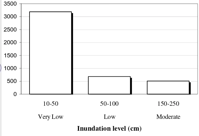
Figure 4.3 shows that the prediction of inundation level in 2030, are in range 10 cm to 150 cm. The inundation level was then classified into 3 inundation depth levels namely: very low (10~50 cm), low (50~100 cm), and moderate (100~150 cm) as tabulated in Table 4.2. Figure 4.5 shows several inundation levels of landuse type and their corresponding area in 2030.

10-50cm 50-100cm 100-150cm Very low Low Moderate

Building 176.619 87.814 60.745

Residential 855.077 596.383 449.426

Embankment 2155.650 − −

(52)

0 500 1000 1500 2000 2500 3000 3500

10-50 50-100 150-250

Very Low Low Moderate

H

e

c

ta

r

e

Figure 4.5 Graph of Tidal Flood in 2030 Area per Inundation Level

In 2030, it is predicted that 4381.7 hectares of embankment area in 2030 predicted will be inundated. This is because the inundation level predicted by SLCC (Sea Level in Common Condition) will reach more than 2 m.

(2100)

SLCC = 0.405 m + 0.316 m + 1.40 m + 2.0112 m

= 4.133 m.

(2100)

SLEC = 0.286 m + 0.714 m + 1.40 m + 4.931 m + 0.40 m

= 4.931 m.

(53)

Based on the sea level prediction in 2100, the inundation level occurred as will have a range between 4.1 m and 4.9 m.

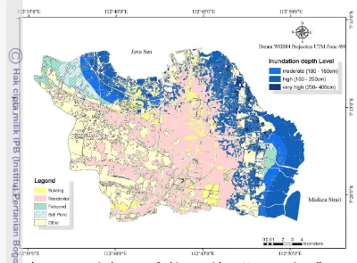
Figure 4.6 Inundation level of Tidal Flood in 2100 per Landuse Class

For the prediction in 2100, the inundation was classified into 3 inundation depth levels namely: moderate (100~150 cm), high (150~250 cm) and very high (250~400 cm). As shown in Figure 4.6 we may conclude, that the inundation in 2100, will reach 25% total area of Surabaya city.

The inundation in 2100 will in range at about 8 km from the coastline. Almost all area in Northern and Eastern Surabaya will be inundated, ranging from 1 to 1.5 m depth. Table 4.3 and Figure 4.7 show several inundation levels of the landuse type and their corresponding area in 2100.

100-150cm 150-250cm 250-400cm Moderate High Very High

Building 306.666 278.685 65.411

Residential 1467.466 1747.302 488.444 Embankment 1500.208 3888.836 −

(54)

0 1000 2000 3000 4000 5000 6000

2010 2030 2100

Ye ar Proje cte d

H

e

c

ta

r

e

Building

Residential

Embankment 0

1000 2000 3000 4000 5000 6000 7000

100-150 150-250 250-400

Moderate High Very High

H

e

c

ta

r

e

Sea level predicted will rise about 2 meters high within 90 years, and if there is no effort to avoid that condition, approximately total 9743 hectares area in 2100 predicted will be inundated. Figure 4.8 is shows trend of the inundation area beyond 2100.

Figure 4.7: Graph of Tidal Flood in 2100 Area per Inundation Level

(55)

4.2 Loss Estimation

From the prediction in 2010, 2030 and 2100, the following are their loss estimation for each landuse type and flood water depth (see Table 4.4 ~ 4.7). Basically the calculation of damage due to floodwater is derived from the costs per ha area.

Table 4.4: Loss estimation of landuse type in relation to the inundation intervals

Prices are given in Indonesian Rupiah (1 USD = 8500 IDR, approximately).

<10 cm 10-50 cm 50-100 cm 100-150 cm 150-400 cm Residential 20.00 300.00 1,000.00 1,600.00 2,000.00 Warehouse Building 0.00 400.00 800.00 1,000.00 2,000.00

Fishpond 0.00 1.13 2.25 4.50 4.50

Saltpond 0.00 0.08 0.15 0.30 0.30

Landuse type Cost damage per Ha (in million idr)

Table 4.5: Estimation loss of landuse type related with inundation level in 2010

<10 cm 10-50 cm 50-100 cm Residential 5,120.24 158,438.40 179,194.00 Warehouse Building 0.00 11,432.00 15,936.00

Fishpond − − −

Saltpond − − −

Landuse type Cost damage (in million idr)

As shown in Table 4.5, estimation of total loss in 2010 is about 370 billion rupiahs. While estimation of total loss in 2030, is about 2 trillion rupiahs (Table 4.6). Then estimation of total loss in 2100 is about 3.6 trillion rupiahs (Table 4.7).

0-50 cm 50-150 cm 150-250 cm Residential 256,523.10 596,383.00 898,852.00 Warehouse Building 70,647.60 70,251.20 121,490.00

Fishpond 1,745.51 − −

Saltpond 45.31 − −

Landuse type Cost damage (in million idr)

0-150 cm 150-250 cm 250-400 cm Residential 2,347,945.60 3,494,604.00 976,888.00 Warehouse Building 306,666.00 557,370.00 130,822.00

Fishpond 939.92 12,913.46 −

Saltpond 199.42 305.75 −

(56)