THE IMPACT OF FREE TRADE AGREEMENTS ON
COMMODITY TRADE FLOWS (CASE STUDY:
INTERNATIONAL PALM OIL TRADE)
RISKA PUJIATI
POSTGRADUATE SCHOOL
BOGOR AGRICULTURAL UNIVERSITY BOGOR
I, Riska Pujiati, hereby declare that the master thesis entitled “The Impact of Free Trade Agreements on Commodity Trade Flows (Case Study: International Palm Oil Trade)” is my original work under the supervision of Advisory Committe and has not been submitted in any form and to another higher education institution. This thesis is submitted independently without having used any other source or means stated therein.
Herewith I passed the thesis copyright to Bogor Agricultural University.
Bogor, September 2014
Riska Pujiati
RISKA PUJIATI. The Impact of Free Trade Agreements on Commodity Trade Flows (Case Study: International Palm Oil Trade). Under Supervision of MUHAMMAD FIRDAUS, ANDRIYONO KILAT ADHI, and BERNHARD BRÜMMER
This study analyzes the impact of Free Trade Agreements (FTAs) on the international palm oil trade for two primary exporters of palm oil: Indonesia and Malaysia. The study used 21 annual observations for 77 export destinations which contain 19 percent zero observations. The gravity model with Ordinary Least Squares (OLS) Fixed Effect (FE) and Poisson Pseudo Maximum Likelihood (PPML) regressions are utilized to quantify the changes of palm oil trade flows. The differentiation of palm oil into crude and refined is used for a deeper analysis of the impact of FTAs. As a result, the PPML estimation provides more satisfactory results than the OLS FE model due to the treatment of zero values data. Variables which influence palm oil export is palm oil production, GDP of destination country, distance, and free trade agreement which established before and after year 2000. The impact of FTAs is shown by the regression results of the different types of palm oil: crude (HS 151110) and
refined (HS 151190). In addition, the estimation output shows that the FTAs have a larger impact on the Malaysian palm oil trade than the Indonesian palm oil trade.
RISKA PUJIATI. Dampak Free Trade Agreements terhadap Aliran Komoditas (Studi Kasus : Perdagangan Minyak Kelapa Sawit Internasional). Di bawah bimbingan MUHAMMAD FIRDAUS, ANDRIYONO KILAT ADHI, dan BERNHARD BRÜMMER
Studi ini menganalisis dampak dari pembentukan Free Trade Agreements (FTAs) terhadap aliran perdagangan minyak kelapa sawit internasional bagi dua exportir terbesar, yaitu : Indonesia dan Malaysia. Studi ini menggunakan data tahunan selama 21 periode dan 77 negara tujuan ekspor dengan data yang tidak memiliki observasi (nol) sebanyak 19 persen. Model gravity dengan regresi Ordinary Least Squares (OLS) Fixed Effect (FE) and Poisson Pseudo Maximum Likelihood (PPML) digunakan untuk mengukur perubahan aliran perdagangan minyak kelapa sawit. Jenis minyak kelapa sawit dalam studi ini dibagi menjadi crude dan refined untuk analisis yang lebih mendalam.
Hasil estimasi menggunakan PPML memberikan hasil yang lebih memuaskan dibandingkan OLS FE berdasarkan perlakuan terhadap data yang memiliki nilai nol. Variables yang berpengaruh terhadap ekspor minyak sawit adalah produksi, GDP Negara tujuan ekspor, dan free trade agreement yang dibentuk
sebelum dan setelah tahun 2000. Dampak dari FTAs ditunjukkan dari hasil regresi terhadap dua jenis minyak sawit yaitu : crude (HS 151110) and refined
(HS 151190). Lebih jauh, hasil estimasi menunjukkan bahwa pembentukan FTAs memberikan dampak yang lebih besar terhadap Malaysia bila dibandingkan Indonesia.
© Copyright belongs to IPB, 2014
All Rights Reserved Law
Prohibited quoting part or all of this paper without including or mentioning the source. The quotation is only for educational purposes, research, scientific writing, preparation of reports, writing criticism, or review an issue; and citations are not detrimental to the interests of IPB.
THE IMPACT OF FREE TRADE AGREEMENTS ON
COMMODITY TRADE FLOWS (CASE STUDY:
INTERNATIONAL PALM OIL TRADE)
RISKA PUJIATI
Master Thesis
as a requirement to obtain a degree Master of Science in Agribusiness Program
POSTGRADUATE SCHOOL
BOGOR AGRICULTURAL UNIVERSITY BOGOR
2014
Name : Riska Pujiati NIM : H451110101
Approved
Advisory Committee,
Prof Dr Muhammad Firdaus, SP, MSi Chairman
Dr Ir Andriyono Kilat Adhi Member
Prof Dr Bernhard Brümmer Member
Agreed,
Coordinator of Major Agribusiness
Prof Dr Ir Rita Nurmalina, MS
Dean of Postgraduate School
Dr Ir Dahrul Syah, MSc Agr
This research would not have been impossible without the support of many people. I would like to appreciate everyone that has assisted me.
First of all, all praise to God, who is most precious and the most merciful for his blessing on all stages of this research process. I would like to acknowledge the support of the National Education Ministry of Indonesia for funding my study in Germany. I am indebted to my first supervisor Prof. Dr. Bernhard Brümmer from the University of Göttingen, Germany who supported me academically in writing this thesis from the beginning until the end. I would also like to thank him for his insight and his constructive criticism of my work.
I would like to thank my supervisor Prof. M. Firdaus and Dr Andriyono K Adhi from Bogor Agricultural University, Indonesia for their evaluation and valuable comments on this research. I would also like to acknowledge Prof. Rita Nurmalina, as the head of the Master Science of Agribusiness.
My sincere thanks to Thomas Kopp in developing this thesis. My special thanks to Katie Wilhelm for proofreading this thesis. My special thanks to Heti Mulyati, Dessy Anggraeni and Manoj KV for their advice on this work.
Furthermore, my thanks to all of my friends and family in the SIA program
and in the Göttingen Indonesian Student Community, especially for the ‘SIA-IPB
Batch 2 and 3”, Maryam, Labudda, Ella, Triana, Puspi, Venty, Angga, Ahmad, Cahya, Eca and my flatmate, Hombe Gowda for providing me a friendly and warm environment during my stay in Göttingen.
Finally, I would like to thank all of the members of “Bapak Haji Edi Djunaedi family” for their love and their support. I dedicate this work to my beloved grandparents, Mr. Edi Djunaedi and Ms. Onyas Rostini, my parents, Mr Agus and Ms. Ika, aunts, uncles and cousins who always give me their love and support.
Bogor, September 2014
Riska Pujiati
LIST OF TABLES xiii
LIST OF FIGURES xiii
LIST OF APPENDIX xiii
LIST OF ABBREVIATIONS xiv
1. INTRODUCTION 1
Background 1
Problem Formulation 2
Research Objective 4
Research Benefit 4
Research Scope 4
2. LITERATURE REVIEW 5
Empirical Studies on Free Trade Agreement Impact 5
The Gravity Model for International Trade 7
Empirical Study on International Palm Oil Trade 8
3. THEORETICAL AND OPERATIONAL FRAMEWORK 9
International Trade Theory and Free Trade Agreement Definitions 9
International Trade Theory 9
Free Trade Agreement Definitions 10
Impact of Free Trade Agreement 11
Static Impact of Free Trade Agreement 11
Dynamic Impact of Free Trade Agreement 13
Theoretical Gravity Model 15
Trade Cost 16
4. RESEARCH METHODOLOGY 19
Data Types and Sources 20
The Gravity Estimation Analysis 20
Ordinary Least Squares: Fixed Effect Estimation 20
Poisson Pseudo Maximum Likelihood Estimation 22
The Regression Specification Error Test (RESET) 24
Econometric Modelling of International Palm Oil Trade 24 5. OVERVIEW OF PALM OIL INDUSTRY AND FTAs IN SOUTHEAST
ASIA 25
History and Policy 25
Plantation Area and Production 27
Palm Oil Export and Import 28
The International Oil Palm Production Chain 30
Current Status of FTAs in Effect in Southeast Asia 31
6. RESULTS AND DISCUSSIONS 35
Trend of Indonesia´s and Malaysia´s Palm Oil Export 35
Conclusion 45
Policy Recommendations 46
1 Major FTAs in Effect in the Asia-Pacific Region 32
2 Status of AFTA and ASEAN+1 FTAs 33
3 OLS and PPML Estimation Result for Palm Oil Export as Dependent
Variable 40
4 PPML Estimation Result for HS1511, HS151110, and HS151190 41 5 The Change of Palm Oil Export due to FTA establishment (%) 42
LIST OF FIGURES
1 Major Commodity Exporter 2
2 Market Shares of Indonesia and Malaysia´s Palm Oil Export 3
3 Trade Creation Effect 10
4 Trade Diversion Effect 11
5 Firm´s Decision to Export based on Trade Costs 15
6 Operational Framework 18
7 Indonesia´s Palm Oil Plantation Area and Production Volume 26 8 Malaysia´s Palm Oil Plantation Area and Production Volume 27
9 Palm Oil Export by Type 28
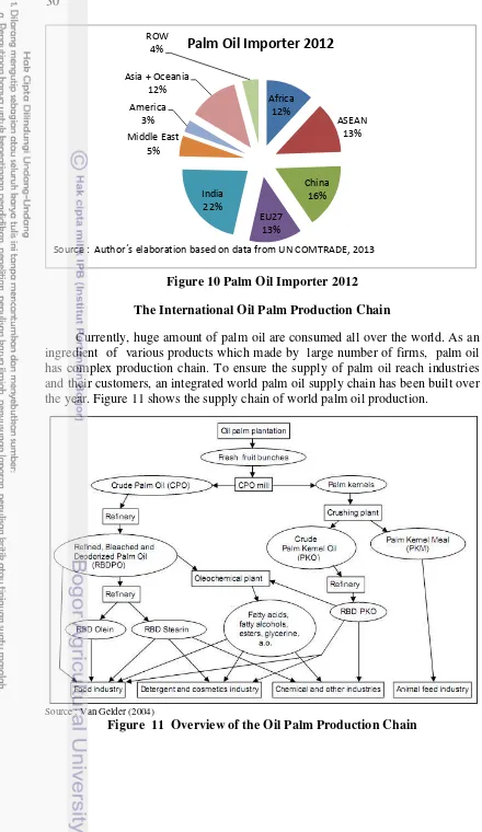
10 Palm Oil Importer 2012 29
11 Overview of the Oil Palm Production Chain 29
12 Indonesia´s Palm Oil Export 35
13 Malaysia´s Crude Palm Oil Export 36
14 Malaysia´s Refined Palm Oil Export 37
LIST OF APPENDIX
1 Derivation of the Anderson and Van Wincoop (2003) Gravity model
Following Bergeijk and Brakman (2010) 51
2 Summary Statistic 52
3 OLS with FTA Dummy united 53
4 Modified Wald test for groupwise heteroskedasticity in fixed effect
ASEAN Association of Southeast Asian Nations ACFTA ASEAN-China Free Trade Area
AFTA ASEAN Free Trade Area
ARIC Asia Regional Integration Centre
AVW Anderson and Van Wincoop Gravity Model CEPII Centre d’Etudes Prospectives et d’Informations
Internationales
COMESA Common Market for Eastern and Southern Africa ECM Error Correction Model
EEC European Economic Community EFTA European Free Trade Association EU European Union
FAO Food and Agriculture Organization of United Nations FELDA Federal Land Development Authority
FFB Fresh Fruit Bunch FTAs Free Trade Agreements GDP Gross Domestic Product
HS Harmonized System
IMP Industrial Master Plan
MERCOSUR Southern Cone Common Market NAFTA North American Free Trade Agreement NBPML Negative Binominal Model
NES Nucleus Estate and smallholder scheme OECD Organisation for Economic Co-operation and
Development
OLS Ordinary Least Squares PPP Purchasing Power Parity
PPML Poisson Pseudo Maximum Likelihood RTA Regional Trade Agreement
RESET Regression Specification Error Test
SITC Standard International Trade Classification
UN COMTRADE United Nations Commodity Trade Statistic Database WITS World Integrated Trade Solution
WTO World Trade Organization
1.
INTRODUCTION
Background
In recent years, international trade has become a complex subject instead of the basic exchange of goods and services that it started out as. Moreover, trade liberalization becomes a critical issue for the trade of goods between countries. During the globalization process, due to the development of communication, technology and transportation, international trade has increased dramatically. The report from the World Trade Organization (WTO) indicates that the total value of worldwide trade is three times larger than it was in the year 2000. As of 2012, international trade is estimated at around US$ 17.9 trillion, whereas it was only approximately US$ 6.4 trillion in 2000. Furthermore, 97 percent of international trade involving the countries which engaged in preferential trade agreement.
Political factor and economic background becoming the reason for a country to establish the agreement. Preferential trade agreement is manifestation of economic integration among countries. The basic principal of integration economic is to eliminate trade barrier and boost the flow of goods and services between its member. The main goal is people´s welfare will be achieved by trade efficiency and reduction in trade cost. Trade policy also set as a tools to create broader market and it is expected to increase a country´s economy growth. The latest development is the establishment of regional trade agreements in each part of the world.
The sectors which contribute to the world trade are agriculture (9.3 percent), fuels and mining (23.1 percent) and manufacturing (64.1 percent). The trade value has increased from US$ 0.5 trillion in 2000 to US$ 1.6 trillion in 2012 for the agriculture sector (World Trade Organization [WTO] 2012). International agricultural trade is important, especially in developing countries. The total share of agricultural exports from developing countries increased slightly over the two decades between 1990 and 2010, from 37 to 43 percent (Cheong et al. 2013). Agriculture plays an important role for developing countries as a primary source of income (Aksoy & Beghin, 2004). In many developing countries, agriculture also becomes a strategic sector which absorbs a high number of employment opportunities. Majority of emerging economy exporting raw agriculture product.
Southeast Asia is a region that consists of middle income developing
economies, with two countries contributing as the region’s major exporters,
Indonesia and Malaysia. In 2012, the value of the total agriculture exports reached US$ 45 billion for Indonesia and US$ 34 billion for Malaysia (WTO 2012). The major commodity which contributes to the high value of export is vegetable oil initially originated from palm oil.
Organization [FAO] 2013). Figure 1 shows the performance of palm oil trade compared to the five largest traded commodities in international market.
The figure 1 shows that the growth of the palm oil trade has increased from 2007 to 2011 for both Indonesia and Malaysia. The average annual growth of Indonesian palm oil was 24%, whereas the average annual growth for Malaysian palm oil was 17%. The total value of exports increased by more than 150 percent in 2011 compared to the value in 2007 for Indonesia, while for Malaysia it increased by only 90 percent. The high growth of palm oil trade is also supported by the increase in palm oil production in both countries.
Figure 1 Major Commodity Exporter Problem Formulation
The extensive use of palm oil in various trade sectors such as the food, non-food and energy sectors led to a high demand of palm oil in the international market. Palm oil is also considered to be the cheapest vegetable oil and has a higher yield than soybean and rapeseed, which are also commonly used to produce vegetable oil. Palm oil is exported in two primary forms: crude and refined. Furthermore, there are more than 100 countries listed as the destination of Indonesian and Malaysian palm oil. Figure 2 shows the palm oil market share for both countries. According to the figure 2, Indonesia and Malaysia have different shares of the palm oil market between the periods of 1989-2012. The European Union (EU) was the primary trading partner of Indonesia with the total market share reach by 82 percent in 1989, this share dropped significantly to 14 percent in 2012. For Malaysia, the share for the EU increased slightly from 8 percent in 1989 to 13 percent in 2012. China is considered to be the new emerging nations, both in
0
economy and population, and is therefore showing a tremendous increase in the import of the palm oil. For palm oil originating from Indonesia, the export share to China reached 15 percent in 2012 compared to three percent in 1989, while for Malaysia, the export share to China reached 17 percent in 2012 compared to 9 percent in 1989. Another country which shows dramatic import increases of palm
oil is India. In 2012, Indonesia’s palm oil export share reached 28 percent while in 1989 the share was only 7 percent. Similar cases apply to Malaysia, where the export share to India reached 15 percent in 2012, three times larger than in 1989 at
only 5 percent. Similar to China and India, the export share of Indonesia’s palm oil to countries grouped to the Association of Southeast Asian Nations (ASEAN) has increased to 14 percent in 2012. Contrary to Malaysia, the export share of Malaysia´s palm oil to ASEAN market decreased from 25 percent in 1989 to 11 percent in 2012.
The change of the palm oil export proportion is influenced in part by the establishment of trade agreements among countries. Indonesia and Malaysia are involved in similar free trade agreements, which are part of the ASEAN Free Trade Area (AFTA) Agreement. During the period between 2000 and 2012, there has been an expansion of partnership with ASEAN; newly added countries are: China (2005), Korea (2007), Japan (2008), India (2010) and Australia/New Zealand (2010).
As two of the largest producers, joining the AFTA become an opportunity for Indonesia and Malaysia to promote trade because of the reduction in trade barriers. Although Indonesia and Malaysia produce similar products, involvement in the RTA will give different results in the flow of goods. Based on the description above, the research question of this study is:
What is the impact of the establishment of FTA on the Indonesian and Malaysian palm oil trade flows, respectively?
Research Objective
According to the research question above, the purpose of this research is to analyze the impact of the establishment of free trade agreements on Indonesia and
Malaysia’s palm oil trade flows.
Research Benefit This study is expected to give benefit as follow :
1. Contribute as a source of information about regional trade and its impact to commodity trade flow for student, researcher, and other related party
2. Give the stakeholder valuable information which can be used as a guidance to take important decision relates to international agricultural trade.
Research Scope
This study is emphasis on Indonesia and Malaysia as a largest palm oil exporter. This study uses disagregate palm oil export which is divided into crude palm oil (HS 151110) and refined palm oil (HS 151190). The value of annual bilateral trade of palm oil is from period between 1991 to 2011 to 77 partner countries as an export destination.
2.
LITERATURE REVIEW
This chapter contains an overview regarding empirical studies which relate to the economic impact of trade agreements, this chapter also looks at previous studies pertaining to the use of the gravity model on international trade, particularly to examine the ex-post effect of the formation of trade agreements. Furthermore, this chapter also describes the international trade of palm oil in Indonesia and Malaysia.
Empirical Studies on Free Trade Agreement Impact
Following the recent proliferation of trade agreements, both bilateral and multilateral, researchers have dedicated efforts to examining the welfare effect of trade agreements. From this increase in interest regarding trade agreements, the question of trade enhancements or the potential generation of threats has arisen. Viner introduced the terms trade creation and trade diversion in 1950; trade creation refers to a shift of product origin from expensive domestic producers to more efficient producers which are a member of trade agreement. Trade diversion occurs when a member country transfers its imported goods from a country that is outside of the trade agreement to a member country within the trade region (Feenstra & Taylor 2008). Trade creation is associated with welfare improvement and trade diversion is welfare reduction. This two concepts serve as the basis for the majority of studies of regionalism and contributes to extensive theoretical literature (Magee 2004).
Research conducted by Aitken (1973) relating to the Regional Trade Agreements used gravity models to look at the differences between European Economic Community (EEC) and the European Free Trade Association (EFTA) to shows that trade creation had occurred between member. Grinols (1984) analyzed the impact that joining the EEC had Britain in 1973. The results indicate that membership in the EEC caused a 2% decline in the Britain`s GDP from 1973 through 1980 (Feenstra 2007).
Korinek and Melatos (2009) conducted the research on the effect of the ASEAN Free Trade Agreement (AFTA), the Common Market for Eastern and Southern Africa (COMESA), and the Southern Cone Common Market (MERCOSUR) in the aggregate agricultural sector. Their results from the gravity model indicate trade creation for member of these agreements, and also displayed no strong proof of trade diversion for countries outside the agreement. Upon the comparison of the result, it can be seen that the the effect on MERCOSUR is larger than the effect on both AFTA and COMESA.
Research performed by Gilbert, et al. (2001) focused on the regional trade in Southeast Asia. Their research on the agriculture, manufacturing, and service sectors shows a positive effect for trade within the agriculture and manufacturing sector. More specific, they conclude that the ASEAN Free Trade Agreement (AFTA) only been boosted the trade in manufacturing through year, while the impact on agriculture declined after 1992. The effect of the AFTA partnership was examined by Yang and Martinez-Zarzoso (2013), through their research on the effect of the ASEAN-China Free Trade Area (ACFTA). The research was conducted with the use of a panel data set from 31 countries from 1995 to 2010. Their research found that the ACFTA has a different impact for each product; there was a significant effect of trade creation applied to manufactured goods and chemical products, while for agricultural raw material, machinery goods and transport equipment, the estimation report insignificant result. Overall, the ACFTA had a positive result on trade among its members and even on countries outside the ACFTA.
Rose (2004) used panel data from 175 countries of the WTO over a 50 year time span (year to year) to determine the implications for a country that is joining a multilateral trade agreement. He concludes that the membership in the WTO has no significant effect on trade. Two possible reason that exist for there being little effect to the member when joining the WTO : First, the WTO cannot force most countries to lower trade barriers, especially for developing countries and second, the WTO membership has little effect on trade policy. Another study was conducted by DeRosa (2007), where he applied the gravity model on a panel data set with annual data from 1970 to 1999 covering 156 countries and 46 preferential trade agreements. The research was conducted on manufacture products and the econometric estimation shows that major preferential trade agreements tend to create trade rather than divert trade. This effect also applied to the non -member countries.
Concerning agricultural commodities, Lambert and McKoy (2009) performed the research on the agricultural and food product on various FTAs. Their research covering three periods of data series, 1995, 2000 and 2004. Their results from the gravity model estimation indicate that FTA generally increases trade in agriculture and trade sector. However, the trade diversion occurred for the members of Caribbean Community and Common Market, the Central American Common Market, and COMESA.
commodities, the FTAs has significant impact to trade on wheat and other cereal gains; and paddy rice.
The Gravity Model for International Trade
The gravity model is one of the most established model for empirical studies in international trade. Over the last decades, the gravity model has successfully explain the determinant of bilateral trade. Moreover the model has been used to asses capital flow, trade resistance, and the impact of regional trade agreements on bilateral trade. The gravity model for international trade derived from the classical gravity model of Newton.
The Gravity model began to be used as a tool to analyze social and economic interaction after the research conducted by Ravenstein in the 19th century. Ravenstein (1885) explains that migration of population is influenced by
the “absorption of centers of commerce and industry, but grow less with the
distance proportionately”. The empirical application of Newton´s gravity model
on international trade was introduced by Tinbergen (1962) in “Shaping the World
Economy”. According to this model, trade between countries is explained by economic sizes, populations, direct geographical distances and a set of dummy variables. Tinbergen concluded that a country´s income and distance have a statistically significant affect on trade between countries.
Gross Domestic Product (GDP) as a measurement for economic country size is an important variable which helps to construct the gravity equation. GDP
indicates the market size in both countries, as a quantifier of ‘economic mass’.
The market size of the importing country represents the potential demand for bilateral imports, while the GDP in the exporting country shows the potential supply and variety of products. Helpman (1987) performed research that stresses the effect of varied country size. His research applied to OECD countries and he concluded that when a country is more similar in size, trade opportunities are expanded. Hummels and Levinsohn (1995) further develop Helpman`s work by including non-OECD member as a means of comparison. Debaere (2002) uses several different methods to determine the share of a country´s GDP, rather than using the nominal GDP, Debaere made these GDP conversions by using nominal exchange rates, as well as Purchasing Power Parity (PPP) exchange rate. Furthermore the research also uses the populations of the countries as an instrumental variable for GDP.
absolute income per capita between trading countries, the second is concerned with kilometers or miles between destinations.
Disdier and Head (2008) estimated the effect of distance through the use of the gravity equation with data comprised of 595 regressions between 1928 to 1995, from 35 separated studies. The result shows that if distance is doubled, then trade will decrease by one half. The effect of distance on regional trade was demonstrated by Martinez-Zarzoso and Lehmann D (2004). They conduct a study focused on MERCOSUR and EU trade. The result shows that for some industries, geographical distance has a high significant effect, this is also true in relation to the economic distance.
Particularly, the gravity model has been augmented by the addition of several critical variables by several author. Common variables which might influence the bilateral trade are common borders, common language, colonial links and the presence of landlocked countries. regarding to the policies impact, the gravity model is widely used to estimate the influence of monetary unions and regional trade agreements.
Empirical Study on International Palm Oil Trade
Extensive research has been conducted to examine the determining factor of palm oil trade in the international market. Suryana (1986), Tondok (1998), Ibrahim (1999), and Basiron (2001) analyzed the outlook of palm oil in the international market for Indonesia and Malaysia. Shamsuddin et al. (1997) examined the determinant and implication of policy instruments on the Indonesian and Malaysian palm oil. Lubis (1994), Shamsuddin et al. (1994), and Susila (1995) who examined Malaysia´s palm oil supply and demand system.
Yulismi and Siregar (2007) calculate the elasticity of price and income for Indonesian and Malaysian palm oil export. The research using annual data from between year 1990 to 2004 analyzed through demand model. The result shows that the price and income elasticity of Indonesian palm oil export are inelastic in India and elastic in China´s market. For the Malaysian palm oil, the price and income are elastic in India and China, while in the EU market the price is elastic.
The impact of the Free Trade Agreements (FTA) proliferation to a country´s overall trade especially palm oil was describe by Ernawati et al.(2006). The export of Indonesian palm oil was analyzed by using an Error Correction Model (ECM), along with having China, India, Europe, and rest of the world (ROW) as partner country. The simulation shows that a reduction of tariff in export and import has varying impacts on partner country. The palm oil demand is influenced by price, as is the price of substituted commodities such as rapeseed oil and soybean oil; exchange rate and lag export, are also shown to be influenced in the simulation.
market share in two regions instead of one, as was the case in Malaysia. Malaysia´s palm oil market share increased only in the Europe region.
Furthermore, another study concerning the impact of FTAs was conducted by (Balu & Ismail 2011). According to their descriptive research, for Malaysia´s palm oil industry, the FTAs were a good opportunity because it helped to increase market share and tariff reduction lead to a higher profit. The competitiveness of traded goods will likely enhance due to liberalization of tariffs.
3.
THEORETICAL AND OPERATIONAL FRAMEWORK
This chapter contains an overview about the theories which support this study. The first part is about the theory of international trade, the second part states the definition of Free Trade Agreements (FTAs) and its static and dynamic impact. The third section explains about the theory development of the gravity model, and the final part gives an overview of trade costs
International Trade Theory and Free Trade Agreement Definitions International Trade Theory
International trade is a part of international economics which refers to “the exchange of goods and services among the countries of the world” (Reinert 2012) The theory of international trade was first developed by British economist, Adam Smith. Smith (1776) stated that trade among nations is influenced by its absolute advantages (Reinert 2012). When a country has the best technology and specialization in the production of one good it has an absolute advantage. The country that has an absolute advantage will gain from export (Feenstra and Taylor 2008).
Ricardo (1821) developed the theory of comparative advantage. This theory state that even if a country has no absolute advantage in producing two types of goods than any other country, the beneficial trade can occur as long as the ratio of prices between countries are different than in an autarky (no trade) situation. As stated by Krugman (2012) “A country has a comparative advantage in producing a good if the opportunity cost of producing that good in terms of other goods is
lower in that country than it is in other countries” (p. 56). The classical trade theory was developed to measure the economic efficiency of resource distribution in the production of goods.
The development of trade patterns proposed by Heckscher (1919) and Ohlin (1924) explained that comparative advantage arises from differences in a country´s endowment factor. The Heckscher Ohlin (HO) theory is also called the factor-proportion theory because it stresses on the interaction between the
different proportions of the country’s production factors, as well as the differences
in the usage of these factors on producing a wide range of items (Krugman,et al. 2012). The assumption of this theory is that the technologies are the same across both trading countries. The HO model predicts that a country tends to export the good which uses its abundant factor intensively (Feenstra & Taylor 2008).
changes into differentiated goods. The market structure in this new trade theory is different than with perfect competition. The concept of monopolistic competition was introduced by Krugman (1980), and states that the two main assumption are differentiated goods and increasing returns to scale. By creating various types of products, firms are able to control the product´s price, the firm also acts as a price taker. In monopolistic competition, a firm cannot set prices as high as in a complete monopoly. The second point of interest is economies of scale. By increasing production, the average cost will be reduced, so the firm will sell more not only in the domestic market, but also in the foreign market. Increasing returns to scale is one of the primary reasons for doing international trade when the trading countries have similar technologies and resources (Feenstra & Taylor 2008). The monopolistic competition model is able to explain current trade patterns such as intra industry trade, the gravity equation, and the impact of regional trade agreements.
The development of the new trade theory by Melitz and Bernard in 2003 focused on the presence and behavior of heterogeneous firms in the international market. The heterogeneity of the firms appears due to not all of the firms being involved in export activities, only several firms are actively exporting. Moreover, not all firms export goods to all countries due to the higher costs involved with the international market than with the domestic market. Hence, only firms which have high productivity are able to cover all costs and export their products. Therefore, the bilateral trade flow may contain many zero values. The presence of zero trade has an important implication on the gravity model.
Free Trade Agreement Definitions
Generally, according to the World Trade Organization (WTO), free trade agreement is “a contractual arrangement between two or more countries under which they give each other preferential market access, usually called free trade. In practice, free-trade agreements tend to allow for all sorts of exceptions, many of them temporary, to cover sensitive products. In some cases, free trade is no more than a longer-term aim, or the agreement represents a form of managed trade liberalization. Researchers have noted that many recent free-trade agreements have run to several hundred pages, whereas a true free-trade agreement would require only a few lines”. While free trade area stand for “a group of two or more countries or economies, customs territories in technical language, that have eliminated tariff and all or most non-tariff measures affecting trade among themselves. Participating countries usually continue to apply their existing tariffs on external goods” (WTO 2003).
Due to the high number of proliferation of regional trade agreement in some part of the world, WTO then define the term of “regional trade agreement” as the
“regional trade arrangement”. The term define as a free-trade agreement, customs union or common market consisting of two or more countries” (WTO 2003). Presently, the number of regional trade arrangement which have been notified to the WTO between 1947 and the present reach more than 200. The WTO established a Committee on Regional Trade Agreements to observe its effect on the international trading system in early 1996.
Impact of Free Trade Agreement Static Impact of Free Trade Agreement
As mentioned in chapter 2, the impact of trade agreements was first introduced by Viner in 1950. Viner’s model is important because it refuses the conventional wisdom of Free Trade Agreements that they tend to improve welfare
because they include some degree of trade liberalization. Viner’s model shows
that a regional trading agreement could have a negative impact on welfare. His model remains important as part of the analytical framework because it lays out several conditions that determine whether an FTAs will be beneficial or harmful. The main concepts in his model are trade creation and trade diversion (Plummer et al. 2010). Both of which counted as the static impact of trade agreement.
The term trade creation indicates the benefit of a country by joining an FTAs. Countries begin to trade with one another, whereas they previously produce all goods internally at a high cost. The definition of trade creation is the converting of imports from a high cost producer to a low cost producer. Contrary to trade creation, trade diversion represents the negative efficiency effect of FTAs, when a country begins to trade, a country which had previously been importing good from a non member with lower production costs must begin importing from a member country with higher production costs due to the establishment of trade agreement (Feenstra & Taylor 2008; Reinert 2012). An illustration of trade creation and trade diversion can be seen in Figure 3.
Figure 3 displays the demand and supply of a certain good in the domestic
market, which is referred to as the “home” country, other FTAs-member
countries are referred to as “partner” countries, and non-member countries as
“outsider.” The assumption for home is a small economy, so that it is unable to
Figure 3 Trade Creation Effect
As an implication of the agreement with Partner, the consumer surplus in the home country increases by a + b + c + d. The producer surplus decreases by a and the government revenue from tariffs are then reduced by c. The net increase as a result of trade creation is b + d. To summarize:
Consumer surplus : a + b + c + d Producer surplus : -a
Government revenue : -c Net welfare : b + d
The change of import which originated with a high cost producer (Home) and was transferred to a low cost producer (Partner) in a trade-creating FTA generates the increasing net welfare in Home. In contrast to Figure 3. Figure 4 illustrates the impact of a trade diverting FTAs. Outsider is now considered to be lowest cost producer, rather than Partner. Then, Poutsider < Ppartner . Due to Poutsider + t < Ppartner + t, prior to the FTAs, Home imports the good from Outsider and the beginning import level is ZHome. When Home joins the FTAs with Partner, however, Ppartner < Poutsider + t, so Home will still transfer its import to the partner country. Import quantity will expand to ZHome,FTAs as the domestic price falls from Poutsider + t to Ppartner.
As a consequence of a FTA with Partner, Home´s consumer surplus increases by a + b + c + d, the producer surplus is reduced by a and the government revenue decreases by c + e. Therefore, the net increase in welfare is b + d – e. To summarize :
Consumer surplus : a + b + c + d Producer surplus : -a
Government revenue : -c + e Net welfare : b + d – e
Quantity
source : Reinert (2012), author´s modification Price
Home Demand Home Supply
ZHome, FTAs
c
b
a
Ppartner Poutsider Poutsider + t
Ppartner+ t
ZHome
source : Reinert (2012), author´s modification
e
Poutsider Ppartner+ t
Poutsider + t
Home Demand Home Supply
ZHome, FTAs
d
c
b
PricePpartner
ZHome
Quantity
Figure 4 Trade Diversion Effect
The net welfare effect is depends on the relative size of b + d + (-e). The area b + d represents trade creating, i.e., the change of import from the higher cost of Home to the lower cost producer of Partner. However, area e denotes the trade diverting effect of changing imports from the lower cost producer (Outsider) to the higher cost producer (Partner). If the trade diverting effect is larger than the trade creating effect (e > b + d), then the FTA reduces welfare in Home (Reinert 2012).
Dynamic Impact of Free Trade Agreement
As has previously been mentioned, in assessing the impact of FTAs, the majority of researchers have focused only on the static (one-time) changes while ignoring the dynamic (medium and long-term) outcomes of FTAs. The dynamic effects of an FTA are important to analyzed because the dynamic effect is more substantial and pervasive (Plummer, et al. 2010); it is necessary to consider what
the FTAs are and how they affect the country’s development. Some of the
important dynamic effects in FTAs to consider are: economies of scale and variety, technology transfer and foreign direct investments (FDI), structural policy change and reforms, as well as competitiveness and long run growth effects. These effects will be discussed in more detail in the following segments.
a. Economies of scale and variety
Economies of scale are described as the reduction in average costs due to an expansion in output. It will occur due to an improvement in technical efficiency in large-scale production, a higher ability to distribute administrative costs and reduce overhead cost over a larger operation, dealers´ bulk discounts or better logistic systems as the production volume increases. Economies of scale occurs
c
a
in the production of some agricultural, natural resource intensive, manufacturing, and service sectors. Due to the establishment of FTAs, the larger market that is created allows firms to take advantage of a larger customer base in domestic and foreign markets. Firms will produce at a lower average cost and are thus able to
set lower prices for existing customers, this is called the “cost reduction effect” (Plummer et al. 2010). As a consequence of lower costs, the firm has a higher competitiveness in both home and foreign markets. Customers in each country will also enjoy a greater variety of goods because the firms in each country will have access to a wider array of goods.
b. Impacts on foreign direct investment
The establishment of FTAs, both bilateral and regional create a more integrated marketplace and a larger risk sharing investment flow. Another benefit for multinational corporations is that they can enjoy a regional division of labour with lower transaction costs, further developing economies of scale. Due to these effects, many multinational corporations are interested in investing more into FTA members due to the dynamic of having a larger economy; this is called
“investment creation.” An FTA may encourage more FDI flows into the region by
working with other multinational countries located outside the region. This is another reason that FTAs may also encourage intra-bloc investments by working with multinational companies of a specific regional origin.
However, if the multinational company chooses to invest in the member country not because of an increase in dynamism but because it will now have preferential access to the FTA market, then it is called an “investment diversion.” Although investing in an outsider country might have higher costs, the multinational company diverts investments to the FTA because of the regional agreement.
c. Structural Policy Change and Reform
Several policiy changes have occurred as a result of the establishments of FTAs. Changes relate to some of the following aspects : quality standards, corporate and public governance laws, customs procedures; the national treatment of partner-country investors, competition policies, the reform of state-owned
enterprises, and other “sensitive sectors” which have an important influence on
the economy. The inclusion of these areas in FTAs shows the extent to which FTA are shaping and harmonizing the member country´s policies. Generally, member country will respond to joining an FTA by improving the business environment through cost reduction, extending the opportunity to join the FTA to foreign investors, and by pushing policy reforms to encompass best practices (Plummer et al. 2010).
d. Competitiveness and Long-Run Growth Effects
The competitive market will give firms a greater incentive to invest in more efficient productive processes and technology. The combination of effects of increased competition on productivity and efficiency will lead to long run growth prospects among member countries. (Plummer et al. 2010).
Theoretical Gravity Model
The basic foundation of the gravity model in international trade is the classical gravity model introduced by Newton. Newton (1686) states that the gravitational attraction between two objects is a function of the mass of each
object and inversely relates to the distance’s square, resulting in the following
formula:
(3.1) =
�
Where F denotes the force between two masses, m1 refers to the mass of the first object, m2 represents the mass of the second object, r shows the distance between two objects, and G is the gravitational constants. If the formula is applied to international trade, F denotes the flow of trade between country i and country j, G is constant, m1 and m2 refer to the a economic size of country i and j, and r represents the distance or trade cost between country i and j. The initial gravity model can expressed as :
(3.2) = � ( )�( )� �
where is the value of bilateral trade (export or import) in current US dollars, and represent exporter and importer´s economic size, is the distance between the two countries, � is the disturbance term, and the βs are the unknown parameters of the equation.
The initial development of the gravity model has presented a degree of problems because the formula is based more on physics than on economic analysis. The gravity equation was not very well appreciated in the decade between 1970 and 1980, due to lacking a strong theoretical foundation in economics. According to Deardorff (1984), the gravity equation has a “theoretical
heritage” which is dubious. In his subsequent research, Deardorff (1998) noted that gravity model can be rationalized with many existing trade theory such as the Ricardian and the HO models, as well as with monopolistic competition.
Anderson (1979) was the first who established a microeconomic foundation for the gravity model. In Anderson´s theory the goods are differentiated by their origin. However, Anderson´s model was not really recognized by trade economists (Head & Mayer 2013). The next theoretical foundation of the gravity equation set by Bergstrand (1985, 1989) who developed a connection between endowment factors and the bilateral trade model. Bergstrand (1989) shows that the gravity model is a practical example of the monopolistic competition theory as developed by Krugman in 1980.
The renowned work of Anderson and Van Wincoop (2003) “gravity with
and has been completed by many other researchers. Principally, the Anderson and Van Wincoop (AVW) gravity model originated from a demand function. The structure of the model was based on the final formula of the constant elasticity of substitution equation for consumer preferences. Consumers have “love of variety”, by consuming a greater variety of goods, the overall utility increases. The second assumption of the AVW gravity model follows Krugman´s (1980) production function; under the condition of increasing returns to scale, each firm produces one particular product. The large number of firms diminish the competition, the price is constant and can cover firm the firm´s marginal costs and fixed costs. In international trade, trade cost´s regularly occur and become somewhat of a barrier.
The AVW model shows the importance of controlling relative trade costs. Their results indicate that bilateral trade is influenced by relative trade cost. Country j imports from country i and must pay a price which is influenced by the weighted average trade cost being paid to all other trading partners. The derivation of the AVW model can be seen in the appendix. The cross sectional gravity equation by AVW is summarized below :
(3.3) =� � elasticity of substitution and � represents trade costs. Two important features of the AVW model is the two additional variables, Π and � . Π is called the outward multilateral resistance, and � is called the inward multilateral resistance. The outward multilateral resistance denotes the exports from country i to country j depending on trade costs across all possible export markets. The inward multilateral resistance denotes the imports into country i from country j depending on trade costs across all possible suppliers (Shepherd 2013). Generally, these figures are low if a country is isolated from world market (Bacchetta 2012). Inward multilateral resistance is also called the price index and outward multilateral resistance is called competition (Fally 2012).
Trade Cost
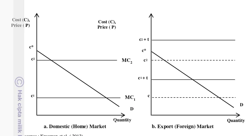
Figure 5 Firm´s Decision to Export based on Trade Costs
It is assumed that the firm must set an extra cost (t) for every unit of output which it sells to the buyer through the country´s border. The firm´s behavior in the domestic and export markets are analysed separately. Accordingly, the firm will set a different price for the domestic and export markets, this will lead to the difference in profit due to the quantities sold in each market. Taking into consideration that the firm´s marginal cost is constant, the firm´s decision to sell in domestic market will have no effect on the export market in terms of pricing and quantity sold.
There are two assumption that need to be considered for explain trade cost: First, there are two firms that both exist in the home country, and second, both countries are identical in consumer preference and technologies. Both firms face a similar demand curve in the foreign country as well as in the home country. The marginal cost in the foreign country is higher than in the home country, the line shifts upward from c1 to c1 + t for Firm 1 . For Firm 2, the cost shifts upward from c2 to c2 + t. In accordance with a previous explanation, the higher the marginal cost, the more a firms is encourage to raise its price, further reducing the quantity sold, and thus lowering profits. If the marginal cost is higher than c*, the firm cannot operate effectively in that market due to a loss in profitability.
The presence of trade costs in the gravity equation are modelled as “iceberg
cost”. This term is used to explain that not all of goods that are shipped will arrive
at the destination. The goods that do not arrive at the destination are considered to have been lost (or melted) in transit. Definitely, if the CIF value is used to measure imports, trade flows are reduced by transport costs (Bacchetta 2012). Following the Anderson & Van Wincoop (2003) model, Shepherd (2013) has derived the trade cost equation from the firm`s marginal cost equation :
(3.5) � = �
� − �
where � shows the variable cost, represents the wage rate, � represents country, and � denotes the firm´s sector. The terms in brackets are a constant markup within the sector, because the numerator must be larger than the denominator. Thus, there will be a positive wedge between the price at the firm´s factory gate and its marginal cost. Since the wedge is influenced by the sectoral elasticity of substitution, it remains constant for all firms within the sector.
This is true when a firm ships goods from country i to country j, it must send � ≥ units in order for a single unit to arrive. The difference is seen as
“melting” (like an iceberg) towards the destination. At the same time the marginal
cost of producing one unit of a good in country i that is subsequently consumed in country i is � , but if the same product were to be consumed in country j then the marginal cost is instead � � . Hence, costless trade gives � = , and � corresponds to one plus the ad valorem tariff rate. Since the size of the trade friction associated with a given iceberg coefficient does not depend on the quantity of goods shipped, the iceberg costs are treated as variable (not fixed) costs.
Using two countries i and j, the incidence of iceberg trade costs occuring means that the price of goods in country j that are produced in country i is determined as follows :
(3.6) � = �
� − � � = � �
In a more general form, a country´s price index it can be written as follows:
(3.7) � = {∫�∈� [� � ] −� } −�
In the above equation, the index includes varieties in goods that are produced and consumed in the same country: each � terms is set to a point of unity, that can indicate the absence of internal trade barriers.
bilateral trade flow for crude and refined palm oil. As a largest producer and exporter, Indonesia and Malaysia has different way to utilized the trade agreement to raise their own market and profit. The operational framework of this study can be seen on Figure 6.
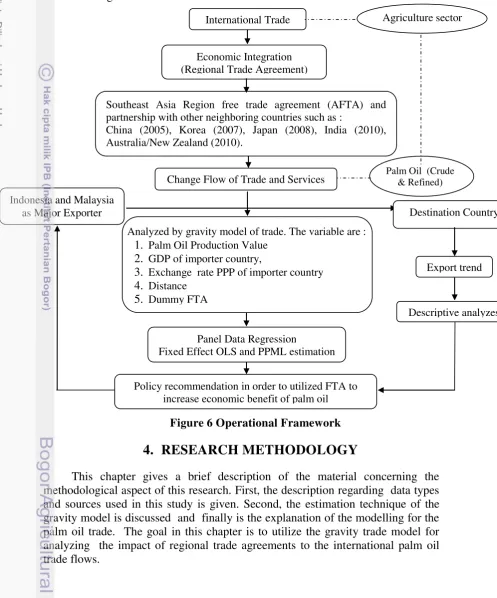
Figure 6 Operational Framework
4.
RESEARCH METHODOLOGY
This chapter gives a brief description of the material concerning the methodological aspect of this research. First, the description regarding data types and sources used in this study is given. Second, the estimation technique of the gravity model is discussed and finally is the explanation of the modelling for the palm oil trade. The goal in this chapter is to utilize the gravity trade model for analyzing the impact of regional trade agreements to the international palm oil trade flows.
Change Flow of Trade and Services Palm Oil (Crude & Refined) Indonesia and Malaysia
as Major Exporter
Analyzed by gravity model of trade. The variable are : 1. Palm Oil Production Value
2. GDP of importer country,
3. Exchange rate PPP of importer country 4. Distance
5. Dummy FTA
Policy recommendation in order to utilized FTA to increase economic benefit of palm oil
Panel Data Regression
Fixed Effect OLS and PPML estimation
Agriculture sector
Southeast Asia Region free trade agreement (AFTA) and partnership with other neighboring countries such as :
China (2005), Korea (2007), Japan (2008), India (2010), Australia/New Zealand (2010).
Economic Integration (Regional Trade Agreement)
International Trade
Destination Country
Export trend
Data Types and Sources
This study uses secondary data available from various sources. The bilateral trade of palm oil annual data from the period between 1991 and 2011 has been generated from the United Nations Commodity Trade Statistic Database (UN COMTRADE) and further incorporated with the World Integrated Trade Solution (WITS) software. The data consists of a nominal value of bilateral trade from Indonesia and Malaysia to 77 partner countries that have conducted trade more than ten times within the 21 year period. The total palm oil and its fraction which has Harmonized System (HS) code: 1511 differentiated into crude palm oil, HS code: 151110 and refined palm oil but no chemically modified HS code: 151190. The geographical distance between countries was obtained from the Centre d’Etudes Prospectives et d’Informations Internationales (CEPII), crude oil price obtained from three sources, they are Dated Brent, West Texas Intermediate, and Dubai Fateh, the GDP of importer countries and the exchange rate of Purchasing Power Parity (PPP) data came from the World Bank, along with FTA information from the Asia Regional Integration Centre (ARIC). The value of palm oil production is generated from the FAO.
The Gravity Estimation Analysis
The gravity model estimation is utilized to analyze the research question of whether the regional trade agreement influences trade flow or not. The software used for the data processing in this study is STATA 12.
Ordinary Least Squares: Fixed Effect Estimation
Ordinary Least Squares (OLS) estimation has been widely used to estimate the gravity equation. The basic form of the multiplicative gravity model is as following:
(4.1) = � � ( � )� ( )� � ��
Taking the natural logarithm, the baseline a log linear gravity model is as follows:
(4.2) ln = + ln � + ln � + ln + � +
where denotes the export value from country i to j, subscript i refers to the exporter, while subscript j refers to the importer, D denotes the distance between countries and FTA is a binary variable assuming a value of 1 if i and j has a free trade agreement and 0 otherwise, is the error term.
The objective of OLS is to obtain the value of by minimizing the sum of square errors (Gujarati, 2011) The OLS estimation has to fulfill the following criteria to become the best and efficient estimator :
b. The variance of the error term must remain constant (homoskedastic)
c. There must be no perfect linear relationships among explanatory variable (no multicolinearity assumption)
If all three properties are fulfilled, then the OLS estimator is consistent, unbiased, and efficient. A consistent estimator means that the OLS coefficient estimation converges to population value when the sample size increases, unbiased means that the estimators are equal to their true values, and efficient means that there is no other estimation than OLS which has a minimum variance of standard error.
Furthermore, the use of panel data and panel econometrics in the gravity model show an increasing trend. According to Baltagi (2009), panel data can control individual heterogeneity, give more informative data, give a stronger degree of freedom and efficiency, and is less likely to have problems with autocorrelation and multicolinearity than time series data. Panel data also deals with time invariant omitted variable.
There are two estimation techniques for panel data, the fixed effect (FE) and random effect technique. The fixed effect model assumes that individual heterogeneity is captured by the intercept term which means that every individual has his own intercept while the coefficients along the slope remain the same. The fixed effect is also known as the Least Square Dummy Variable due to the use of a dummy variable (Gujarati, 2011). The fixed effects model has been used in the majority of gravity estimation studies over the last decade and tends to provide better results (Kepaptsoglou, et al., 2010).
Concerning the unobservable multilateral resistance terms (MRTs), the fixed effect technique can be used to control these MRTs1. Anderson and Van Wincoop (2003) emphasized that the MRTs should be taken into account in order to avoid a biased estimation of the model parameter. Fixed effect is applied by put the dummy of country specific and country pair into the estimation. Country specific dummy variables are used to capture all of the time invariant individual effects of exporters and importers that are excluded from the model specification such as preferences, institutional differences, etc. Country pair dummies are used to address the bias due to the correlation between the bilateral trade barriers and the multilateral resistance. Furthermore, the time dummy variable will take into account to control for macroeconomic effects such as the global economic recession. The equation considering individual country specific effects, country pair effects and time effects is specified as:
(4.3) ln �= + ln ��+ ln ��+ ln + � +
� + + � + �+ �
where � denotes export value from country i to j at time t, stands for the fixed effect of country i (exporter fixed effects), � represents the fixed effect of country j (importer fixed effects), � denotes country pair fixed effects, and � refers to the time effect.
According to Baier and Bergstrand (2007), one important econometric issue that arises when estimating the impact of FTAs is endogeneity. The problem arises due to the correlation between FTAs terms with the error term �). Many researchers wrongly assume that the FTAs is an exogenous random variable (Yang & Martinez-Zarzoso 2013), for example, a country´s decision to join a trade agreement is not related to unobservable factors. Following the hypotheses
of “natural trading partner” as proposed by Krugman (1991), the countries prefer to have trade agreements with partners who already have high value trade. Baier and Bergstrand (2007) also noticed that the FTA is not the only cause of bilateral trade, but other unobserved factor such as non-tariff barriers, democratic relationship, infrastructure and institutional characteristics also play a role. The research by Baier and Bergstrand (2009) verified that a country´s decision to join an FTAs depends largely on their economic size and the difference in factor endowments.
The endogeneity problem can be solved in several ways. Baier and Bergstrand (2007) argue that instrumental variable can be applied to solve the endogeneity, but it is not easy to find appropriate variables for FTA. They suggest using country-and-time effects and country pair fixed effects. Baldwin and Taglioni (2006) suggest that applying time varying country dummy variables can counteract the endogenous bias, Martínez-Zarzoso et al. (2009) suggest using country specific dummy variables in cross sectional data and bilateral fixed effects to remove the endogenous bias.
Poisson Pseudo Maximum Likelihood Estimation
Several things need to be taken into consideration when using the gravity model to analyze disaggregated data, the first being the presence of zero trade. In sectoral trade, zero values appear more frequently than with aggregate data. There are two possible causes for zero trade, first, the high cost of transport due to excessive distances and trading partners having small economy. Second, are the consequences of firms self-selecting to export to a particular destination due to high fixed costs (Bacchetta 2012).
The zero value will automatically be dropped when using the OLS method, the implication of dropping the zero is that the useful information will be lost which will further lead to inconsistent result (Bacchetta 2012). There are three main approaches to dealing with zero trade. The first option is an ad hoc solution which is done by adding a small value (0.0001) to the trade data, so the zero is defined by log (0.0001) and then the tobit estimation is used after this process. However, the ad hoc solution has no basic statistical theory. The second commonly used approach is the Poisson model, and the third is the Heckman model.
heteroskedasticity, the result from the PPML estimation will provide better result by including the zero value rather than truncating OLS.
The PPML estimator has several properties which are desired for analyzing the impact of policies (Shepherd 2013). First, it is consistent with the existence of fixed effects; second, the Poisson estimator will include zero value observations, and third, the interpretation of the PPML is directly follows the OLS. The subsequent research by Santos Silva and Tenreyro (2011) shows that the PPML is consistent and performs well in the presence of over dispersion (the conditional variance is not equal to the conditional mean) and excess zero values. The use of PPML and Poisson family regression models such as the zero-inflated poisson model, (ZIPPML), negative binominal model (NBPML), and zero-inflated negative binominal model (ZINBPML) in disaggregate data, especially in singe trade commodity has increased. Following Burger et al. (2009), the assumption for bilateral trade flow between countries i and j has a Poisson distribution with the conditional mean � �, which is a function of the independent variables. As is assumed to have a non-negative integer value, the exponent of the independent variable is captured in order to assure that � is zero or positive. The PPML estimation takes the following form:
(4.4) Pr[ ] =exp(−� )�
�
� ! , = , , , …
where the conditional mean � is connected to an exponential function of a group of regression variables, ´
. � = exp + ´ + + � )
where is constant, is the 1 x k row vector of the explanatory variables that correspond to the parameter vector which represents trade barriers, is the exporter effect, � is the importer effect. The assumption of this model is equi dispersion; the conditional variance of the dependent variable is equal to its conditional mean.
Sun and Reed (2010) was the first author who applied PPML on the effect of FTAs with disaggregated data for agriculture commodities. The result of PPML is superior to the OLS result. Following Sun and Reed (2010), the empirical model is specified as:
(4.6) � = exp{ + ln ��+ ln ��+ ln + � +
� + + � + �+ �}
The Regression Specification Error Test (RESET)
Ramsey (1969), introduced the regression specification error test (RESET) to check the significance of the regression of a residual on a linear function. This is done by assuming an approximation vector of mean residuals from the least-squares estimate of the dependent variable and a ranking of the squared residuals. RESET then basically checks whether the regression of the residual vector against its rank is significant or not. This is why this test is also famously known as a rank correlation test.
RESET is generally used to test the specification of a linear regression model by examining whether or not a non-linear combination of the fitted values can help with explaining the dependent variable. If the non-linear combination of the dependent variable is statistically significant, then the model is misspecified. The model is explained with the following equations:
(4.7) ŷ = { | } = �
The RESET Ramsey test then examines whether � , � ,.., � has any influence on . This is performed by estimate the equation as follows:
(4.8) = + ŷ +. . . + − ŷ +
afterwards, the significance of through − is determined through the use of an F-test. The null hypothesis is that the coefficient is equal to zero. If the null hypothesis is rejected, then the model suffers from misspecification.
Econometric Modelling of International Palm Oil Trade
Estimating the gravity model for a single commodity can lead to biased estimations if the GDP of exporter countries are used as a proxy for the economic size of the exporter �� . Therefore, the production value of palm oil is used
in this study as a proxy for the exporter’s economic size. In order to examine the
impact of free trade, the dummy variable (FTAs) is divided into two parts one before and one for after the year 2000. The main reason for splitting up the dummy variable is the proliferation of FTAs for both Indonesia and Malaysia after 2000, which have become more significant and has additionally expanded with the countries located in Asia region. The list of FTAs can be seen in Chapter 5. The gravity model of international palm oil takes the following form:
(4.9) ln Y t = β + β ln Prodt+ β ln GDPt+ β ln D + β FTAs_early_MYS t+ β FTAs_after_ _MYS t + β FTAs_early_IDN t+
β FTAs_after_ _IDN t+ β ln ppp_cnvrtt + π + + φ + t+ t
(4.10) � = exp{ + ln Prodt+ β ln GDPt+ β ln D +
β FTAs_early_MYS t+ β FTAs_after_ _MYS t + β FTAs_early_IDN t+