Policy, Planning, and Research
1
WORKING PAPERS
Agricultural Policies
Agriculture and Rural Development Department
The World Bank September 1989
WPS 286
Poverty
and
Undernutrition
in Indonesia
during the 1980s
Martin Ravallion
and
Monika Huppi
Because of sustained growth in average real consumption, a
modest improvement in overall equity, and gains to the rural
sector
-particularly the poorest of the poor
-poverty and
undernutrition continued to be alleviated during Indonesia's
recent period of macroeconomic adjustment.
The Policy, Planning, and Research Complcx disuibutes PPR Working Papers to disscminate the fuindings of work in progress and to encourage the exchange of ideas among Bank staff and aU oLhers intcrested in devclopm.ent issues. These papers carry the names of the authors, reflect only their views, and should be used and cited accordingly. The findings, interpretauons, and conclusions are the authors'own. They should not be attributed to the World Bank, its Board of DusrciGrs, its management, or any of its member countnes.
Public Disclosure Authorized
Public Disclosure Authorized
Public Disclosure Authorized
Plc,Planning, sndi Research
Agricultural Pollce
Indonesia adjusted rapidly to sharply falling Although caloric intake data are far from
external terms of trade during the 1980s - ideal, they found evidence that the extent of
using a classic package of currency devaluation, undemutrition also fell significantly. For a
budgetary and monetary restraint, and regulatory caloric intake level which 37 r -rcent of the
relaxation. population failed to attain in 1984, they found
that only 27 percent of the population failed to
How did the rountry fare in its efforts to attain it in 1987.
alleviate poverty and undernutrition during that
period? Why was this so? Gains to the rural sector
contributed greatly to the alleviation of poverty.
It is difficult to measure poverty at one point Gains to the urban sector and population shifts
in time - much less compare poverty in two from the rural to the urban sector also helped but
periods - but Ravallion and Huppi answer that were quantitatively less important than dire
question using two large, comparable sets of gains to the rural poor.
household data for 1984 and 1987. They tested
a wide range of possible poverty lines and Increases in average real consumption and
poverty measures - and the sensitivity of key an improvement in overall equity both helped to
results to many of the underlying assumptions reduce poverty. In addition, Indonesia's recent
about poverty. economic history had created conditions
favor-able to alleviating poverty so long as modest
They found robust evidence that noverty growth in private consumption per capita could
continued to decline during the period. be maintained during the adjustment period.
This paper is a product of the Agricultural Policies Division, Agriculture and Rural Development Department. Copies are available free from the World Bank, 1818 H Street NW, Washington DC 20433. Please contact Cicely Spooner, room N8-039, extension 30464 (54 pages with figures and tables).
The PPR Working Paper Series disseminates the findings of work under way in the Bank's Policy, Planning, and Research | Complex. An objective of the series is to get these findings out quickly, even if presentations are less than fully polished. The findings, interpretations, and conclusions in these papers do not necessarily represent official policy of the Bank.
by
Martin Ravallion and Monika Huppi
Table of Contents
1. Introduction 1
2. Measuring Poverty and Undernutrition 3
3. The Data and Results 7
4. Proximate Causes 12
5. An Alternative Poverty Assessment 18
6. Implications for Future Poverty Alleviation Prospects 20
7. Conclusions 22
Appendix 1: The Distributions 25
Appendix 2: Lorenz Curve Parameterizations 33
v!otes 35
References 42
Tables 46
Figures 52
* This Is the first In a series of papers reporting results of an ongoing World Bank research project, "Policy Analysis and Poverty: Applicable Methods and Case Studies" (675-04), based in the Agricultural Policies Division, Agriculture and Rural Development Department. We are grateful for the financial support and encouragement of the Bank's Research Committee. The paper also provides background support for the 'Indonesia: Poverty Assessment and Strategy Report" being prepared by Asia-Country Department V. The paper has benefited in many ways from the assistance and comments of staff of the Country Department; we are particularly grateful to Kyle Peters and Nicholas Prescott.
We have also had useful comments on the paper from Anne Booth, Francois
Bourguignon, Gaurav Datt, Paul Glewwe, Nanak Kakwanl, Lyn Squire, and Dominique van de Walle. The household level data tapes used here were provided by the Central
Bureau of Statistics, Jakarta. We are most grateful to the Bureau's staff for their
1. Introduction
The 1970s saw a significant decline in the proportion of
Indonesia's population who did not attain minimal nutritional and other consumption needs (Rao, 1984; CBS, 1984). Concern has been expressed about whether this success in poverty alleviation has been sustained through the far more difficult 1980s.1 The various external shocks of the 19809
included sharp falls in the price of the country's main export and source of public revenue, oil. During 1986 alone, this amounted to about a one third
drop in the country's external terms of trade. It is now widely agreed that the government's policy rusponses to these shocks were effective in
stabilizing the main macroeconomic aggregates. However, we know little about their effects on poverty.
Rapid macroeconomic adjustment programs in LDCs can have adverse effects on the poor, and there has been some casual speculation that this may have happened in Indonesia. The public expenditure cuts were certainly
severe; the govornment's total rea± tpenditures fell by about nine percent between 1985/86 and 1986/87. However, a good deal of the immediate burden of adjustment fell on domestic savings and investment rather than private consumption, which did sustain a modest but still positive (per capita) growth rate over the period. Poverty will not increase when mean
consumption is maintained, provided that (and it is an important proviso) the poor do not lose from changes in the distribution of consumption.2
What then happened to Indonesia's distribution of consumption in the 1980s? Existing evidence is inconclusive. It appears that the
be expected to participate disproportionately. Its efficacy in achieving this end is less obvious.3 The currency devaluations and the boom in non-oil exports may have offer-d some protection to the rural sector.4 However, the extent to which this included the rural poor is unclear; while it is plausible that many of Indonesia's rural poor tend to be net producers of tradeable goods (and hence gain from real devaluations), there are also likely to be many poor hou-eholds in both urban end rural areas who are not. There have been reports of a decline in real wage rates in rural Java,
though there ic some conflicting evidence.5
It is also far from obvious that adverse income effects of short-run macroeconomic adjustment on the poor will be reflected in their
consumption. It is not implausible that most of the poor do have strategies of some sort for coping with short-run income declines, such as through adjustments in their labor market behavior, intertemporal consumption behavior and/or their participation in the "moral economy".6 What is less clear, and of greater importance, is how well these coping strategies perform in practice.
This paper examines what happened to aggregate poverty and undernutrition in Indonesia during the period 1984 to 1987. The twin
objectives are: i) to describe empirically how poverty and undernutrition changed over this period, and ii) to examine the proximate causes of those changes. In pursuing both objectives we also hope to illustrate the
paper's main empirical results are presented in Section 3 where we give poverty assessments for various indicators of the standard of living of the poor. While the primary objective of this paper is to measure and describe how poverty and undernutrition in Indonesia changed over this period, it is of interest to go at least slightly further into the causes of those
changes. Section 4 attempts to do this by asking what contributions
sectoral gains and population shifts (on the one hand), economic growth and changes in inequality (on the other) made to aggregate poverty alleviation. The importance of Indonesia's favorable distributional parameters at che beginning of the period is also discussed. Section 5 uses the results of Section 4 to make an alternative assessment of how poverty changed over the period. The alternative method does not assume that the levels of household consumption are comparable across the two data sets. In the light of the paper's results, Section 6 discusses Indonesia's prospects for future poverty alleviation. Section 7 offers some conclusions.
2. MeasurinR Poverty and Undernutrition
A fundamental question which arises when assessing poverty is that of how an individual's "standard of living" is to be measured. Individuals and the states of their environments will differ in many ways which might be deemed relevant in principle, but are not quantifiable. A similar comment applies to measures of undernutrition, where variability in nutrient
aspect of living standard). The problem we face now is how to compare distributions of that measure which, in this instance, are the observed
survey distributions at two dates.
There is now a large theoretical literature on the measurement of poverty, establishing a number of desirable properties for such measures.7
The popular "headcount index" satisfies very few of those properties. There has been much recent interest in a class of measures proposed by Foster, Greer and Thorbecke (FGT) (1984). This is a single parameter index which can be made to satisfy the main axioms of poverty measurement through a suitable choice of that parameter. Each member of the FGT class of poverty measures is identified by the value taken by the parameter a and the
corresponding measure is denoted Pa.8 Three members of the FGT class are considered in this study:
*i) The FGT poverty measure for a 0. This is simply the headcount index, given by the proportion of the population with a standard of living below the poverty line. Thus, if forty percent of the population are deemed to be poor then Po = 0.4.
(ii) The poverty measure for a = 1. This is the average poverty gap in the population, expressed as a proportion of the poverty line. Thus a value of P1 = 0.1 means that, when the aggregate
deficit of the poor relative to the poverty line is averaged over all households (whether poor or not), it represents 10 percent of the poverty line.
(iii) The measure for a = 2. This is a distributionally sensitive measure, based on the sum of the squared poverty gaps of the
-5-'Transfer Axiom" which requires that when a transfer is made from a poor person to someone un is poorer, the measure indicates a decrease in aggrega- poverty. In view of the
desirable properties of this meaaure we shall simply refer to it as our "preferred measure".
However, whilc the search for better cardinal measures of poverty and undernutrition has advanced far over the last fifteen years or so, there is still widespread concern about arbitrariness in the choice of a poverty line, or nutrition cut-off point, and in the choice of a specific functional form for the poverty measure. For example, the popular FGT measure P2
discussed above uses only one of a number of possible functional forms that might be suggested, all satisfying the main axioms for a desirable poverty measure (Atkinson, 1987). Fortunately, for many (though not all) of the purposes of measurement, including some policy analyses, all that one is really concerned about is the ordinal ranking of distributions in terms of poverty or undernutrition. For example, the main question of interest may be: did poverty increase as a result of (say) structural adjustment? As a rule, one will be able to answer this question with much less information, including fewer arbitrary assumptions, than are needed for making the
cardinal comparison: how much has poverty changed?
Rather than confine ourselves to a particular poverty line and poverty measure, we shall draw on recent results on the use of dominance conditions in ordering income or expenditure distributions in terms of poverty.9 For this purpose one can consider a very broad class of poverty measures, which encompass the main contenders found in the literature. And,
are continuous, separable, symmetric and weakly monotonic), poverty will have unambiguously fallen between two dates if the cumulative distribution
of income for the latter date lies nowhere above that for the former date, over the entire interval up to the maximum allowable poverty line (Atkinson, 1987, Condition IA). This is called the first-order dominance test. If the result of that test is ambiguous, then we know that different poverty lines and/or measures will rank the distributions differently; some will indicate a decrease in poverty while others will not. When such ambiguity exists according to the first-order dominance test, then stronger (higher order) dominance conditions may prove useful. Sen's Transfer Axiom is an important example of the sorts of further conditions which may then prove to be
revealing in deciding whether poverty has gone up o down. When applied to the poverty measure, this axiom yields the second-order dominance test which basically requires that the area under the cumulative distribution function up to the maximum poverty line is greater (or no less) over the entire range of admissible lines (see Atkinson, 1987, Condition IIA).
A similar approach can be used to assess changes in the extent of undernutrition, when (as is certainly the case) there is uncertainty about nutritional requirements and their interpersonal distribution. Provided that the interpersonal distribution of requirements has not changed, first-order dominance of the caloric intake distribution for one date over another
implies an unambiguous change in the aggregate headcount index of
more undernourished persons, such as those discussed by Kakwani (1988) and Ravallion (1988b). We shall only attempt to make ordinal comparisons of undernutrition, following the dominance approach.
3. The Data and Results
The SUSENAS tapes give data on household consumption (from both market expenditures and own production) for 50,000 randomly sampled
households at each date. Following past practice for Indonesia, we shall mainly base our poverty assessments on distributions of household
consumption per person, adjusted to February 1984 urban prices using the Consumer Price Index (CPI). The CPI is far from ideal for our purposes.
The index is only constructed for urban areas and its composition is
inappropriate for the poor. We have, however, re-weighted the CPI so as to better reflect the conaumption pattern of the poor, and have also built an
allowance for urban-rural price differentials into the index.10 Appendix 1 discusses the data and their limitations in greater detail. For present purposes, the most worrying features of these data are the possibility that
the rate of inflation in rural areas may be underestimated by the CPI and that SUSENAS data imply a growth rate of real private consumption per capita which is higher than implied by the national accounts. We shall return to these points later.
1984). Results are presented here for the two main poverty lines: a 1984 expenditure of Rp 11,000 per month per person and one of Rp 15,000. The lower povert) line is chosen to :orrespond to that used in past Bank studies, after adjusting for inflation (Rao, 1984, 1986). We take this to be the preferred poverty line.
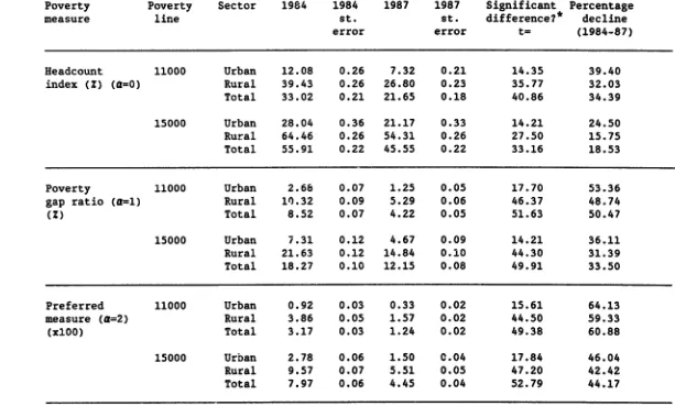
Table 1 gives our cardinal estimates of poverty in Indonesia for various poverty measures and for both poverty lines. All three measures
(including the preferred "distributionally sensitive" measure) and both poverty lines indicate a significant decrease in poverty for both urban and rural sectors.
For the lower poverty line we find that the proportion of the population who are poor decreased from about one in three at the beginning of the period, to slightly over one in five by 1987; this is a substantial contraction over just three years. The corresponding absolute number of poor persons declined from 52 million to 36 million. The poverty gap measure implies that the aggregate consumption shortfall of the poor
declined from about Rp 937 per month per head of Indonesia's population (representing about 5.5 percent of national mean consumption) to Rp 464 in 1987 (about 2.3 percent of the national mean). Such calculations are, however, contingent on the precise poverty line chosen. The higher poverty line in Table 1 also ir.dicates significant declines in poverty, though the numbers are a good deal less dramatic.
9
-al'. possible poverty lines will show an unambiguous decrease in aggregate
poverty between the two dater This was found to hold for both urban and rural areas.
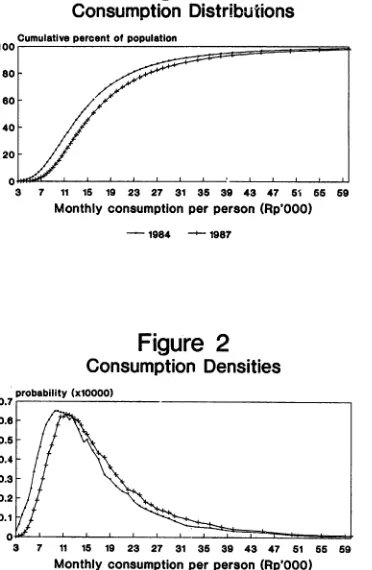
From Figure 1 we can also assess the sensitivity of this conclusion to possible underestimation of price increases facing the poor. The 1987 poverty line (in 1984 prices) which would be needed for the 1987 headcount index of poverty to equal that in 1a84 is Rp 12,818. Thus, an additional inflation rate of at least 16.5 percentage points (on top of the CPI based estimate of about 20 percent) would have been needed over the three years to reverse the conclusion that poverty has decreased by this measure.
Similarly, the true inflation rate would need to be about 14.1 points higher over the three years to equalize the headcount indices for the two dates at the higher poverty line. Thus the conclusion that poverty has decreased would be robust to even quite substantial measurement error in the CPI; the
inflation rate would need to have been underestimated by at least 50 percent to reverse our conclusion.
A potentially important observation about the results in Figure 1 is that the poverty lines are found on a steep segment of the consumption distribution. This is illustrated more clearly by the density function of consumption given in Figure 2. (This is a non-pararatric estimate using a Gaussian kernel). The lower poverty line is very close to the mode, where the slope of the comsumption distribution function reaches its maximum. This has two implications of interest here:
i) Estimates of the headcount index of poverty will be
particularly sensitive to the exact location of the poverty line, as our comparison of the lower and upper poverty lines in Table 1 has suggested.
mode, the response of the headcount index to an additive gain or loss at all consumption levels will be at its maximum. As the results of the following
section will demonstrate, the response of poverty in Indonesia to
multiplicative shifts (in the form of distributionally neutral changes in the mean) was also high in the mid-1980s. This will be seen to have implications for understanding the effects of recent economic growth on poverty.
Is our qualitative result on the change in poverty over this period robust to the choice of an indicator of the standard of living? Three
alternatives will be considered: income, food expenditure share, and caloric intake.
Figure 3 gives the distributions of household income per person. A comparison of the entire frequency distribution again reveals that the
first-order dominance condition holds. No matter where one draws the poverty line, or what poverty measure one uses (within a broad class), aggregate poverty in terms of incomes unambigiously fell between 1984 and 1987. This conclusion is also robust to even substantial measurement error in the CPI.
Keeping in mind the problems of comparing surveyed consumption and income levels over time, it is of interest to consider another alternative measure of the standard of living. It is well known that a household's
apportionment of consumption expenditure between food and non-food goods is an indicator of that household's real consumption level; the share devoted
relative prices, demographic factors and tastes. Differences in relative prices and (possibly) tastes between urban and rural areas could well be the most important factor mitigating the welfare interpretation of
inter-household differences in food shares in Indonesia. For this reason it is probably better to consider urban and rural areas separately.
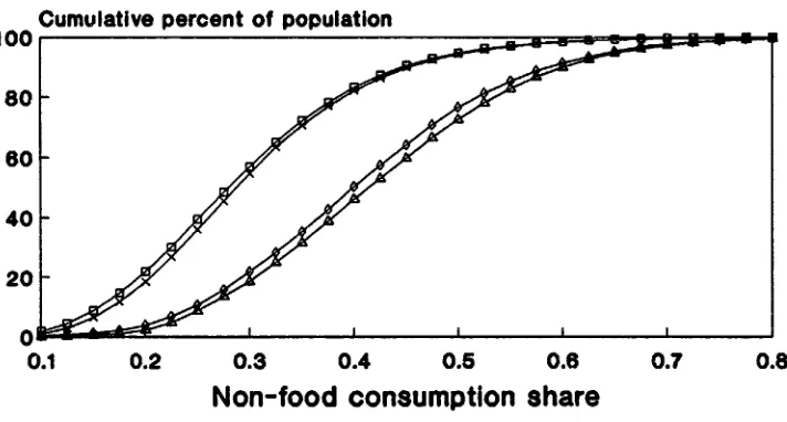
Figure 4 gives the cumulative frequency distributions of the share of non-food goods in total consumption for each of urban and rural areas for each date. First-order dominance still holds up to high non-food shares, so a wide range of poverty lines and measures will continue to indicate a
decrease in poverty in both sectors over this period. The proportion of the rural population with a food share in excess of 75 percent (a commonly used poverty line) fell from 39.2 percent in 1984 to 35.8 percent in 1987, while for the urban sector it fell from 10.5 to 8.5 percent. The decline is not as dramatic as that suggested by the CPI adjusted consumptio. and income data, but it is still evident in the distribution of food shares.
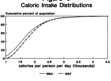
Did undernutrition also diminish? Figure 5 gives the distributions of calorie intake per person for the two dates. The 1987 distribution lies below that for 1984 up to a high intake level (the ranking only reverses for the upper nine percent of persons). First-order dominance thus holds up to high caloric norms. The "second-order dominance condition" discussed in Section 2 holds over the entire distribution, so that it can be concluded that a broad class of undernutrition measures show an improvement whatever the underlying distribution of requirements. These results were also found to hold in both urban and rural areas. The quantitative shift in the
caloric intake distribution is quite substantial at the lower end; for
4. Prozimate Causes
We do not intend to go very deeply here into the reasons for Indonesia's evident success at alleviating poverty during a period of macroeconomic adjustment. But some clues are offered by the following
statistical decompositions of the reduction in aggregate poverty. Sectoral Gains and Population Shifts
The results of Section 3 indicate siCnificant poverty alleviation in both urban and rural sectors. There was also a shift in population over the period, with a declining share in the poorer rural sector (the
proportion of the population living in rural areas fell from 76.5Z in 1984 to 73.6Z in 1987). 'What was the relative contribution of these factors to
the reduction in poverty?
Using the Pa class of poverty measure, the change in aggregate poverty between the two dates can be decomposed into sectoral gains, population shifts, and interaction effects, as follows:
87 84 87 84 84 87 84 84
87 Pa = (Pau - Pau)nu + (Par - Par)nr
gain to urban gain to rural sector at 1984 sector at 1984 population share population share
r87 84 84 r 87 84 87 84
+ E(n8 _ ni
)Pai
+£(Pai
- Pai )(ni - ni ) (1)i-u i=u
gain due to aggregate interaction population shifts effects between sectoral at 1984 sectoral gains and population poverty levels shifts
- 13
-t
at date t (t-1984,1987), with corresponding population share ni. The aggregate interaction effect can be interpreted as a measure of the correlation between population shifts and changes in poverty.
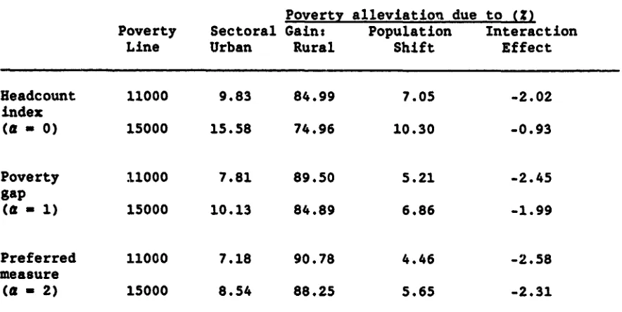
Using this formula, Table 2 gives the urban/rural decomposition of the aggregate poverty alleviation gains. For the headcount index, using the lower poverty line, we find that about 10 percent of the aggregate reduction
in poverty was due to a lower prevalance of poverty amongst the urban sector (while accounting for about one quarter of the population). On the other hand, 85 percent was due to the lower rural poverty, while about 7 percent was due to the higher urban population share. The net interaction effect is
-2 percent.
It can be seen from Table 2 that both population shifts and gains to the urban sector made positive contributions to aggregate poverty
alleviation during the period for all measures, and were dampened only slightly by the negative interaction effect. The quantitative importance of the sectoral gains to rural households is notable, particularly when the measure focuses more on the poorest of the poor (a-2). The gains to this
sector accounted for the vast majority of aggregate poverty alleviation, and generally more than the sector's population share (there is one exception for the headcount index at the higher poverty line). Lower poverty lines and monotonic poverty measures tend to enhance considerably the importance
of gains to that sector; at the lower poverty line and for the preferred poverty measure, the gains to the rural sector represented over 90 percent of the aggregate gain.
in the SUSENAS, giving 21 distinct sources for each of urban and rural areas (Huppi and Ravallion, 1989). Significant reductions in all poverty measures (generally at least as high as the sector means) were experienced by the poorest rural subsectors, notably farm laborers and self-employed farm
households. While 11 and 57 percent of all rural persons in the sample were principally employed in these two subsectors respectively, they accounted
for 17 and 61 percent of the aggregate drop in the preferred poverty measure using the lower poverty line (Huppi and Ravallion, 1989).
Growth, Inequality and Poverty
An alternative way to decompose the poverty alleviation gain is in
terms of the parameters of the aggregate consumption distribution. Roughly speaking, one can identify two proximate causes of a change in poverty: a change in the mean consumption level at given inequality, and a change in the inequality of consumption around the mean; the former can be thought of as the 'growth effect on poverty" while the latter is the "distributional effect"1l. However, the qualitative effect on poverty of a reduction in inequality at a given mean is not obvious a priori; for example, while a transfer of income from someone at the poverty line (or only slightly above it) to someone well below will reduce inequality, it will also increase the headcount index of poverty.
- 15
-denote th., poverty level that one would have found in 1987 if only the Lorenz curve had shifted since 1984, leaving the mean unchanged. The observed change in poverty between two dates can then be decomposed into
"growth" and "distributional" effects as follows: 87 84 87* 84 87** 84
pa
-Pa.(Pa _pa
) +(pa _ Pa) +residual (2)change in change in poverty due poverty due to change in to shift in the mean the Lorenz holding 1984 curve holding Lorenz curve 1984 mean constant constant
However, one should be cautious in drawing policy implications from this decomposition. Distributionally neutral growth is not the same thing as growth with distributionally neutral policies. The laizze-faire growth path of an economy need not be distributionally neutral, and so policy interventions aimed at reducing relevant inequalities may well be essential to attaining even distributionally neutral growth. The "growth-equity" decomposition is a simple descriptive devise intended to throw light on the proximate causes of poverty alleviation; a deeper analysis of those causes would be needed to draw sound policy implications.
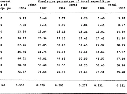
aggregate Gini coefficient (for example) dropped from 0.331 in 1984 to 0.321 in 1987.14
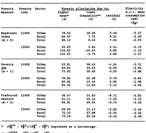
Table 4 gives our estimates of the relative contributions to poverty alleviation of growth and greater equity, using the decomposition formula in equation (2).15 The shifts in the Lorenz curve contributed to poverty alleviation in almost all cases; the exception for rural areas using the higher poverty line is probably due to the fact that the rural mean for 1984 was actually slightly below that poverty line.1 6 In all cases
considered in Table 4, the majority of the reduction in poverty can be attributed to higher mean consumption at given relative consumptions; the contribution of greater equity (upward shifts in the Lorenz curve) is small for the headcount index, though it accounts for a far higher proportion of the change in the preferred measure of poverty.
It is of interest to also consider the point elasticity of poverty in 1984 to distributionally neutral growth. Following Kanbur (1987a) and Kakwani (1989b), it can be readily shown that the elasticity of the Pa poverty measure w.r.t. the mean of the distribution, holding the Lorenz curve constant is given by:
Va = -zf(z)/P0 < 0 (for a = 0)
= a(l - Pa-l/Pa) < 0 (for a > 1) (3)
where f(z) denotes the probability density of consumption at the poverty line z. This also has to be estimated; details can be found in Appendix 2.
- 17
-line and in urban areas. For a given poverty line and sector, the growth elasticity is highest for the preferred measure oi poverty and lowest for the headcount index.
On the Role of Initial Conditions
The results in Table 4 suggest that, by the beginning of the
adjustment period, aggregate poverty in Indonesia was ready to respond quite elastically to any further economic growth. Initial conditions of the
period may thus have been favorable to maintaining the momentum of poverty alleviation, in spite of lower growth. We now investigate that conjecture more closely.
The growth elasticity of poverty is a function of the parameters of the underlying consumption distribution.17 Consider first the mean.
Differentiating (3) with respect to the mean is, it can be readily verified that:
e, = _
Po/
< 0 (for a = O)(a - la-i)aPa-l (for a 2 1) (4)
,UPa
The last derivative is not necessarily negative for all a > 1, though it is found to be so for a = 1, 2, for these data (Table 4). This result can be
Under plausible assumptions about how the Lorenz curves have
shifted over time, it can also be shown that, for these data, the (absolute) elasticity of the FGT class of poverty measures with respect to the mean
(again holding the Lorenz curve constant) is a monotonic decreasing function of the initial Gini measure of inequality;1 8 differentiating (3) with
respect to the Gini coefficient G oae finds that (analogously to (4)):
8-G ' OIIO / G > 0 (for a = 0)
(E a - Ea-1)aP al
-ea QGP > 0 (for a > 1) (5)
where Ea denotes the elasticity of the Pa poverty measure to Lorenz dominating changes in the Gini coefficient.
It can thus be argued that a past history of fairly equitable
growth (resulting in a relatively "high" mean and "low" inequality) resulted in a 'high' elasticity of poverty to future growth in Indonesia. The growth experience over the 1970s and early 1980s would appear to have created a sound foundation for maintaining poverty alleviation from the more modest growth of the mid-1980s. This finding also has implications for Indonesia's poverty alleviation prospects after 1987, as will be considered further in Section 6.
5. An Alternative Poverty Assessment.
- 19
-the three years for -the former as opposed to 5 percent for the latter. The reason for this large discrepancy is quite unclear, and there does not appear to be any sound basis for deciding which is closer to the truth.
However, the results of Tables 3 and 4 also allow us to make an alternative assessment of how poverty changed during the period, avoiding the potentially contentious issues concerning the comparability of the levels of SUSENAS expenditures across the two dates. For this purpose we can use the SUSENAS to assess how overall inequality changed during the period. This assumes that the samples at both dates were representative of the populations, though this seems plausible (see Appendix 1 for further discussion). From Table 3 we can then conclude that there was no
deterioration in overall inequality; indeed equity improved slightly and in
a way which would have reduced poverty. This use of the SUSENAS data
requires comparisons of consumption or income relativities across dates, not absolute levels. Since inequality did not increase, any positive growth in per capita consumption would (as a rule) have reduced poverty (and, indeed,
since inequality fell slightly, a modest contraction in mean consumption would have been possible without an increase in poverty). From the point elasticity estimates in Table 4, the national accounts' growth rate for consumption per capita implies that the headcount index at the lower poverty
6. Implications for Future Poverty Alleviation Prospects
Naturally we cannot say anything with similar confidence about what has happened to poverty in Indonesia since early 1987 (the last available
SUSENAS survey), or what is likely to happen in the future. But some aspects of the methodology we have used here can throw light on the issue. Our 1987 results also allow us to estimate the elasticities of poverty to any future distributionally neutral growth in mean consumption, in a similar manner to those we have used in the 1984-87 analyses. We find that the 1987
growth elasticities are also high; and, indeed, higher than those for 1984. For example, our estimates are -4.1 for the 1987 elasticity of the poverty gap measure with respect to mean consumption using the lower poverty line
(as compared to -2.9 for 1984 from Table 4); similarly, for our preferred measure we obtain an elasticity of -4.8 (-3.4 for 1984). Furthermore, from
national accounts for 1987 and 1988 it appears that growth rates of real consumption per capita have increased. Both these factors - the higher
growth elasticities of poverty and the higher growth rates - imply
increasing poverty alleviation through any distributionally neutral growth since early 1987.
Sustainable future consumption growth in Indonesia will clearly require that investment is revived, after the cuts of the mid 1980s. But it is possible for the poverty alleviation benefits of even substantial
consumption growth to be lost entirely through a sufficient contemporaneous deterioration in overall equity. As we have seen, there was a modest
- 21
-The sharp increase in rice prices during 1987 and 1988 (associated with poor harvests and a reluctance by the government to import rice) is probably the main recent event which could mitigate continued poverty alleviation. The effect on aggregate poverty of higher rice prices is not obvious. Ravallion and van de Walle (1988) found for Java in 1981 that even if rice price increases were allowed to be passed on fully to the incomes of the (typically poor) rice producers, all distributionally sensitive poverty measures would respond adversel' to higher rice prices. The effects are, however, ambiguous for other mfasures of poverty which are not sensitive to the welfare of the poorest of the poor, such as the headcount index. Still, the latter measure is known to be inadequate, and the preferred measures favor a presumption that higher rice prices will (ceteris paribus) increase poverty. It remains to be seen whether adverse effects on the poor of
changing relative prices have been sufficient in size, or persistent enough, to seriously jeopardize continued poverty alleviation through growth in Indonesia.
7. Conclusions
The measurement of poverty at one point in time is fraught with difficultv, and the comparison of two points in time adds even further problems. We have followed past work on poverty in Indonesia and elsewhere in basing poverty measures on distributions of household consumption per person. We have adjusted for inflation using the Consumer Price Index,
though we have modified the underlying expenditure weights to accord more closely to spending patterns of the poor. Recognizing the uncertainties involved in poverty measurement, an effort has been made to use a wider range of both poverty measures and poverty lines. Here we have drawn on insights from the recent literature on poverty analysis using dominance conditions to establish partial orderings of distributions.
From our comparisons of income and consumption distributions over time we conclude that aggregate poverty in Indonesia decreased over the period 1984 to 1987. This holds for both urban and rural areas. In a
neighborhood of commonly assumed poverty lines for Indonesia, the magnitude of the decline in poverty over the period is impressive; 22 percent of the population are identified as poor in 1987 using a consumption poverty line for which 33 percent were poor in 1984. Such numbers can, however, be quite sensitive to how poverty is measured, particularly the choice of a poverty line: for example, 46 percent are deemed to be poor in 1987 using a poverty line for which 56 percent were poor in 1984. But, we find that the
- 23
-levelsl Underestimation in the rate of inflation over the period would need, in our view, to be implausibly high to alter the conclusion that poverty decreased.
A significant (though less dramatic) decline in poverty in both urban and rural areas is also indicated if one uses the share of total consumption devoted to non-food goods as the indicator of welfare, thus avoiding the problems of adjusting for inflation. The proportion of the population who devoted three-quarters or more of their total consumption to food fell from 32 percent to 28 percent over the period. Furthermore, our qualitative conclusions are robust to relaxing the assumption that the household level consumption data are even level comparable across dates; poverty is also found to have decreased (though again by a less dramatic margin than CPI adjusted consumptions indicate) if one bases the comparisons of mean consumptions solely on national accounts, only using the household level data tapes to compare relative consumptions at any one date.
Though the caloric intake data is less than ideal (with some underestimation being likely at both dates), there is strong evidence that the extent of undernutrition also fell significantly. This holds for both urban and rural sectors, over a very wide range of alternative measures of undernutrition and it holds for any (unknown) interpersonal distribution of nutritional requirements, provided that this did not also change over the period. The shift in the caloric intake distribution was far from
negligible at its lower end; we find, for example, that 27 percent of the 1987 population did not attain a caloric intake which 37 percent bad failed to reach in 1984.
poverty and undernutrition in Indonesia continued to decline during the difficult 1980s.
We have investigated the "proximate causes" of Indonesia's success using two methods of decomposition, one based on sectors, the other based on distributional parameters. The sectoral decomposition of the change in aggregate poverty indicates that gains to the rural sector were very
important, particularly for the poorest of the poor. Gains to the urban sector and population shifts between sectors (from rural to urban)
contributed to poverty alleviation, but were quantitatively less important than the direct gains to the rural poor. In terms of the parameters of the aggregate consumption distributions, we found that both increases in average real consumption (holding relative inequalities constant), and a modest improvement in overall equity, contributed to poverty alleviation during the period. The former factor was quantitatively more important, though less so
for the preferred (distributionally sensitive) poverty measure.
A tadk for future research is to understand more deeply how this success was achieved. Some possible clues have been identified here. The gains to the rural farm sector were crucial and so policy adjustments aimed at protecting that sector probably had an important role. Certain
ingredients of the macroeconomic policy response probably helped here, such as the devaluations. Indonesia's recent economic history had a role too; by the mid 1980s, past growth at relatively low inequality had created a
situation whereby relatively large effects on aggregate poverty could be generated by seemingly small shifts in the distribution of consumption. Thus, Indonesia's recent econoric history had created initial conditions for the adjustment which were quite favorable to maintaining the country's momentum in poverty alleviation, provided that at least modest growth in
- 25
-Appendix 1: The Distributions
The Household Consumption and Caloric Intake Data
Past poverty assessments for Indonesia have generally been based on the distributions of household consumption per person from the SUSENAS expenditure surveys done by the Central Bureau of Statistics. We follow this method, though noting that it has both advantages and disadvantages. The following points should be particularly noted:
(i) The SUSENAS is widely recognized as a household consumption survey of relatively high quality which has used sound and consistent survey methods over many years. The 1984 and 1987 surveys appear to be fully comparable in terms of the questions asked, and the methods of sampling and interviewing. The
estimates obtained will depend in part on the date of interview, particularly in rural areas where past work has found evidence of seasonality in consumption (as well as incomes).1 9 The 1984 and 1987 SUSENAS surveys used here were done at approximately the same time of year (February and January respectively) in comparable agricultural years,20 and so this is unlikely to be a problem for comparisons between those years.
(ii) The SUSENAS has the advantage over expenditure surveys fer a rumber of developing countries that it is a consumption based
survey i.e., it does not just ask how much was spent on variuus goods and services, but also asks how much was actually consumed from various sources, including of course, market expenditure but also including consumption from own production and transfers
(iii) Normalizing household consumption by the number of persons makes no allowance for the likely variation in consumption needs
between different persons, according to (for example) age or gender. There is a large literature on the construction of equivalence scales which allow the normalization to take account of such differences in household composition, though it remains that there is no single ideal method of dealing with this
issue.2 1 Future work on measuring poverty in Indonesia might fruitfully address this issue, but for present purposes we shall
follow past practice.
(iv) The use of consumption rather than income is generally desirable in th's setting, since incomes fluctuate more and households can save. It can be argued that consumption expenditures for a single date will provide a better measure of a household's standard of living than current income. However, it is also of interest to examine the effects on incomes, as this is where many of the immediate consequences of macroeconomic adjustment are felt.22
(v) The SUSENAS aims to provide a random sample of the entire
- 27
-assessment of poverty in 1987, relative to 1984. The sampla was stratified spatially. All our calculation have used the local expansion factors (inverse sampling rates) in aggregation. (vi) The SUSENAS is the only available source of data on household
consumption and income in Indonesia which provides national coverage. It is thus essential for constructing consumption or income distributions such as required for convincingly measuring
inequality, poverty or undernutrition. There is another important data source for the national aggregates, such as consumption, notably the national accounts. However, the two
sources do not generally agree on the aggregates; the SUSENAS typically yields lower estimates of mean consumption than the national accounts (see, for example, Dapice, 1980). The reason
for this is unclear. It is thought to be plausible that the SUSENAS undereports consumption, though it can also be argued that this is more likely to be so for the rich than the poor, in which case poverty assessments may still be reasonably
(vii) Income or expenditure based poverty assessments typically ignore publicly provided goods, as these cannot be easily valued in
terms of money. Though there is little hard evidence, there have been numerous casual observations that the mid and late
19808 witnessed a deterioration in the availability and quality of some publicly provided goods for which the poor are amongst the beneficiaries, such as piped water supply, health services, nutrition programs anid schooling. Public services to the poor
are clearly relevant to poverty assessments, but they are unlikely to be reflected in the consumption expenditure distributions used in the present study.
(viii) The SUSENAS estimates household caloric intake by applying fixed caloric food values to observed consumptions of about 170
catagories of food and beverage for each household, based on 7 day recall by the respondent. Caloric intakes are almost certainly underestimated, mainly because consumption of food in
street-side stalls and restaurants is underestimated (such expenditures being classified elsewhere in the survey where physical consumptions are not asked; see van de Walle, 1988). This is more likely to bias the urban caloric distributions than those for rural areas. However, there is no obvious reason why the problem should bias our comparisons over time.
The Price Deflator
- 29
-differences in prices at one point in time may be just as important as the usual intertemporal differences associated with inflation (though the former have generally been ignored in past work.) The consumer price index (CPI)
for Indonesia monitors price changes over time for bundles of goods which are predetermined in composition for each of a number of cities (spanning the archipellego), but are not, however, strictly comparable between
cities.2 4 Nor can it be convincingly argued that the differences in goods composition across regions solely reflect consumer substitution effects. It is quite likely that the bundle of goods is more "generous" in richer
cities; the implicit reference utility level cannot be assumed to be constant.25
Without an ideal price deflator, we have based all distributional comparisons on two alternatives: i) the Ordinary CPI which ignores spatial price variability in the base period, and simply adjusts prices for January 1987 in each province to the corresponding February 1984 prices using the price index for its capital city (although with higher weights on food
expenditure; see below), and ii) the Spatial CPI which uses the expenditure data by city underlying the CPI to construct an index which allows all 1987 consumptions to be expressed in 1984 Jakarta prices. The first index is likely to lead us to overestimate the regional disparities in living
There are two possible problems with the CPI:
(i) The goods composition of the index is not ideal for measuring the standard of living of the poor; the weight on food
(particularly rice) is undoubtedly too low (see, for example, Mulijanto, 1988). This does not, of course, mean that the CPI will underestimate inflation for the poor; that also depends on how relative prices changed. On disaggregating the CPI by
commodity group we have found that the rate of inflation between February 1984 and January 1987 was slightly higher for the food group than the non-food group in most provinces, though the difference is small. There is, however, no reason why one need be confined to the expenditure weights implicit in the CPI. For the purposes of this study we have recalculated the price index using a higher food share, given by the average expenditure
share for the poorest 30 percent of urban households in 1984 which Bank staff have calculated to be 0.68 (certainly a good deal higher than the CPI weight of about 0.45). Since the relative price of food changed little during the study period we do not, however, expect that this re-weighting will have much effect.
- 31
-compared monthly rice prices implied by the CPI with those for a specific grade of rice over recent years. The results suggest that the recent rates of rice price increase for an
approximately uniform quality of rice are higher than those implicit in the CPI. However the divergence has mainly occured since mid-1987, seemingly associated (for some unknown reason) with high rates of rice price increase as a result of that year's poor harvest. The implicit rice price in the CPI tracks well the monthly market price of a uniform quality of rice over
the period of the present study.
Prices also vary between urban and rural areas. Past practice has been to make some assumption kbout the urban/rural cost-of-living
differential, reflecting the fact that the prices for most goods
(particularly food and housing) tend to be higher in urban areas. For example, on Indonesia's most populous island, Java, it has been estimated that average dwelling rents in 1981 were six times greater in urban areas than rural areas, while the price of the main food staple, rice, was on average 10 percent higher in urban areas (van de Walle, 1989a).
Observations of this sort have often led some past investigators to use substantially different poverty lines for urban and rural areas of
Indonesia. This practice has important implications for sectoral rankings in terms of the headcount index of poverty (given by the proportion of the population below the poverty line). For example, the 66 percent
differential in poverty lines between urban and rural areas for 1981 assumed by a past CBS study is sufficient to reverse the poverty ranking of sectors in terms of the headcount index (over that obtained at a zero
A proper treatm%it of these issues would require a demand system analysis to construct a true spatial cost-of-living index. This is beyond the resources of the present enquiry. Nonetheless we can still learn something from recent research along these lines. One of the potentially most important lessons is that past work appears to have considerably overestimated the urban-rural cost-of-living differential for Indonesia.2 8 A differential of about 10 percent appears to be plausible for the poor.2 9 This is assumed. We also assume that the urban-rural cost-of-living differential did not change over the period. This is consistent with the only price index constructed on a comparable basis for both urban and rural areas, namely the CBS Nine Essential Commodities (NEC) index. This also gives a very similar rate of inflation to the CPI, namely about 20-25 percent over this period.3 0 Huppi and Ravallion (1989) discuss the
- 33
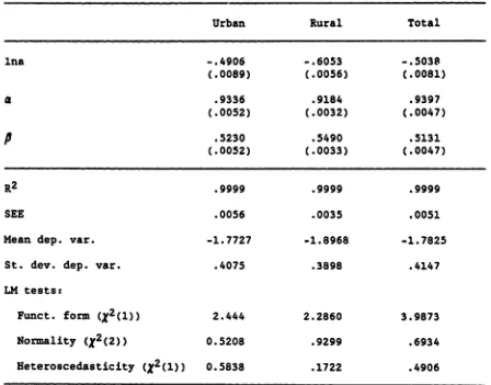
-Appendix 2% Lorenz Curve Parameterizations
The decomposition of poverty alleviation gains into "growth and equity' components in Section 4 uses the following parameterization of the 1984 Lorenz curve (following Kakwani, 1989b):
L(p) = p- apa (lp)PeV (Al) where L(p) is the proportion of total expenditure by the poorest p
proportion of the population and a, a and fl are positive parameters to be
estimated (with convexity of the Lorenz curve requiring that neither a nor
p
exceed unity) and v is a random error process. The P17* poverty measures in equation (2) are then calculated from the parameterizea 1984 Lorenz curve and the 1987 mean, using the formulae given in Datt and Ravallion (1989).Similarly, P&7** is estimated using the parameterized 1987 Lorenz curve and the 1984 mean. The density at any point can also be retrieved from the parameterized Lorenz curve and the mean of the distribution, noting that
f(x) = l/QjL"(p)) where p = F(x) is the cumulative distribution function and
i is the mean. This allows estimation of the growth elasticity
'o
(equation 3). The parameters of the Lorenz curve are estimated from the following linear regression implied by (Al):log[p-L(p)] = log a + a log p +
8
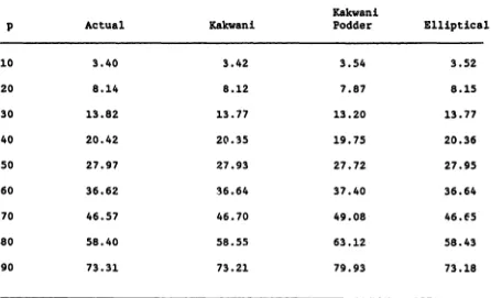
log(l-p) + v (A2)The accuracy of these methods depends on the precision in estimating the underlying Lorenz curve. Table 5 gives the estimated parameters of
percentage SPSints, equivalent to about 0.3 percent of the consumption share
of the poorest half of the population. We experimented with two alternative parameterizations, namely the Kakwani-Podder Lorenz curve and the elliptical Lorenz curve (Villasenor and Arnold, 1989). The corresponding estimates are given in Table 6. The Kakwani Lorenz curve is clearly superior in fit to the Kakwani Podder specification (though that is unsurprising since the latter uses one less parameter). The ranking of the Kakwani and elliptical models is less clear; the latter gives a slightly better overall fit (the standard deviation of the error drops to 0.070). However, the gain is largely due to the elliptical model's better fit in some higher deciles, particularly the eight; Kakwani's model generally fits better at the lower end (for example, standard deviations of the errors for the poorest 50
percent are 0.047 and 0.065 for Kakwani and elliptical models respectively), and so it will generally be more accurate for simulating the poverty
- 35
-Notes
1. Though little convincing evidence has been presented, concerns about adverse effects on the poor have often been expressed in casual
discussions and in recent literature; see, for example. Jayasuriya and Manning (1988), Sundrum (1988), Booth and Sundrum (1988) and Papanek (1988). The latter paper gives evidence that real wage rates in rural Java declined during the 1980s (as discussed further below), while national income per capita was increasing. Papanek infers from this that the overall distribution of income worsened, though that inference is clearly rather hazardous, as it ignores the numerous other variables which influence income distribution. More direct evidence is called
for.
2. There have been recent signs of a slight downward trend in inequality. CBS (1988, Table 10.2.7) reports Gini coefficients for per capita
expenditures of .33 for 1984, .32 for 1981, .34 for 1980, .38 for 1978 and .34 for 1976. However, Lorenz dominance does not hold, so other
inequality measures may give different results. (The conditions necessary for lower inequality to reduce poverty are discussed further
later in this paper). Inequality seems to have been on a rising trend through most of the 1970s; see Fields (1989).
3. See Demery and Addison (1987), and Keuning and Thorbecke (1989). 4. Agriculture accounted for over half of the rise in non-oil exports
between 1986 and 1987; see Baik Indonesia (1988).
end date of Papanek's series tends to exaggerate the downward trend (as it coincided with a severe drought and unusually high rice prices). Nonetheless, his data do suggest declining real wages over the
adjustment period. Collier et al. (1988) do not confirm this result in their study of 13 villages in the same provinces over a similar period. though the two studies have used different price deflators. It may also be noted that labor market adjustment will probably mitigate adverse effects on poor net consumers of tradeable goods, though that adjustment can be slow; for evidence in a possibly not dissimilar setting see
Ravallion (1989a).
6. For evidence on the performance of voluntary redistributive or social insurance arrangements (the so-called "moral economy") in this setting see Ravallion and Dearden (1988).
7. For an excellent survey see Foster (1984).
8. More, formally, for a population of size n, split into m subgroups with population shares ni (i-l,...,m), the FGT class of poverty measures takes the general from
m
P
Pa- n
which is simply the population weighted mean of the subgroup poverty index (Pai), given by:
PaiE E jni for a > 0
- 37
-9. Important contributions are Atkinson (1987) and Foster and Shorrocks (1988).
10. Though a suitable demand model does not exist to allow us to estimate true cost-of-living indices, we have considered some of the implications of consumer substitution possibilities in response to temporal and
spatial differences in relative prices. There is mounting empirical evidence to suggest that those responses are far from negligible for the poor, and substantial errors can arise in using fixed weight price
indices when relative prices vary. See Appendix 1 for further discussion and references.
11. Sundrum (1987, Ch.6), Ravallion (1988a), Kakwani (1989b). In principle, a distributional change around a given mean may alter measured poverty in a way which one would not identify as a change in "inequality". In practice a two parameter characterization is often adequate.
12. More precisely, this will hold for any inequality measure which
satisfies the Pigou-Dalton "transfer principle", namely that a transfer of income (or expenditure) from person A to person B will increase inequality whenever A has lower income than B. See Atkinson (1970). 13. Allowing fur regional price differentials will probably give lower
overall inequality; for example, the Lorenz curve for 1984 based on our estimates of real expenditures using a spatial CPI (see Appendix 1) lies entirely above the Lorenz curve based on nominal expenditures for that year. It appears that regional price levels tend to be positively correlated with average consumptions. A similar conclusion was reached by van de Walle (1989).
data. The distributions were, however, detailed (51 groups) so the approximations should be quite good. In calculating the Gini indices we have used Gastwirth's formulae for the upper and lower boundc and then used the weighted mean of the two, with two-thirds weight to the upper
bound; see Cowell (1977).
15. The P47* and pI7** mepsures are simulated from the parametized 1984 and 1987 Lorenz curves for urban and rural areas, as discussed in Appendix 2, which also outlines our estimation method for qo.
16. This interpretation isn only strictly valid if the Lorenz curve shifts such that L87(p) = L8 4(p) - X[p-L8 4(p)], where Lt(p) denotes the Lorenz curve for date t; then a decrease in the Gini coefficient will decrease poverty (for a broad class of additive measures) if ard only if the poverty line is less than the mean (Kakwani, 1989b). Noting that
X
is equal to the proportionate change in the Gini index, the aboveassumption implies the following national Lorenz curve for 1987 (where '= -.0302):
p 10 20 30 40 50 60 70 80 90
L87 (p) 3.60 8.50 14.31 21.01 28.64 37.33 47.28 59.05 73.81
Clearly this is quite a good approximation to the actual Lorenz curve
for that year (given in the last column if Tablc 3; the standard error
of estimate is 0.23 percentage points), but it is still an
approximation.
- 39
-interest, though they have received little attention. For related discussion see Ravallion (1988c) and Datt and Ravallion (1989).
18. This assumes that the changes in G are such that the new Lorenz curve is
g.,en by L(p) - X[p - L(p)]. As nGted, this assumption fits the data in
Table 4 well (footnote 16). Then 60 = to(z - p)/z and
e =?a + UIAPa.-1/(ZPa) for a > 1, and it is readily verified from the
following formulae that 8va/8G > 0 (all a) for these data.
19. This was found by Ravallion (1988a) in a study of poverty in East Java based on the 1981 SUSENAS which (unlike 1984 and 1987) spanned an entire year.
20. Though harvests in 1987 were depleted, this occurred after the SUSENAS interviews.
21. For a recent discussion and some evidence for Indonesia see Deaton and Muellbauer (1986).
22. Noting that the distribution of consumption will also depend on how households adjust in their intertemporal behavior.
23. There is some evidence of a systematic bias, whereby the "poor" tend to overestimate food expenditure over a 7 day recall, while the "rich" underestimate it. The turning point (at which there is neither under-or overestimation on average) is such that standard poverty measures for Indonesia will tend to be underestimated, though the magnitude of the error is probably farily small. For detailed results and an
interpretation see (Ravallion (1989b).
24. The index tracks changes in the cost of an average consumption bundle in each of 17 Provincial capital cities; for other capital cities they have used shares for the city amongst the 17 which is considered to be most
25. Nicholas Prescott pointed this problem out to us in his comments on an earlier version. We considered an alternative deflation method, using
the Department of Manpower's 'Minimum Physical Requirements Index" (KFM) which is intended to be a cost-of-living index for working households,
and is derived independently of the CPI. We studied this index closely, including a discussion with the Department of Manpower officers
responsible for the index. For a number of reasons we decided that the index is quite unsuitable for our purposes. Details are available from the authors.
26. For the lower poverty line, the headcount index obtained using the spatial CPI drops from 34.70 percent in 1984 to 23.47 percent in 1987, while for the higher poverty line, the corresponding figures are 58.96 and 47.62. As for the ordinary CPI, first-order dominance holds over the entire range.
27. The study referred to is CBS (1984). For further discussion see Ravallion and van de Walle (1989).
28. Though it may be argued that real consumption "standards" are higher in urban areas, and so a higher real poverty line is called for. This is, in our view, difficult to defend on ethical grounds; we take it as axiomatic here that poverty comparisons should be symmetric, in the
sense that the poverty line in terms of real living standards (leaving aside the problems in measuring the latter) should be constant over time and space.
29. See Ravallion and van de Walle (1989). An urban and rural price
- 41
-30 Anne Booth has pointed out to us in correspondence that the consumption component of the "Farmers' Terms of Trade Index* (FTT) for Java does suggest a higher inflation rate for rural areas than the CPI or NEC. However, we have found that this is largely due to the very high price increases recorded for vegetables in the FTT for Central and East Java over 1985-86 (see, for example, CBS, 1987 Table 9.4.9). Substitution possibilities in consumption are thought to be relatively high for vegetables (Deaton's, 1989, estimates for Java in 1981 indicate a
Reference
Atkinson, Anthony B. 1970. "On the Measurement of Inequality." Journal of Economic Theory 2: 244-263.
, 1987. "On the Measurement of Poverty". Econometrica 55:
749-64.
Bank Indonesia. 1988. Laporan Minaguan, Bank Indonesia, Jakarta.
Booth, Anne. 1988. "Survey of Recent Developments." Bulletin of Indonesian Economic StudieR 24:3-36.
Booth, Anne and R. M. Sundrum. 1988. "Employment Trends and Policy Issues for Repelita V", Jakarta: International Labor Organization, Mimeo. Central Bureau of Statistics (Biro Pusat Statistik). 1984. "Indikator
Pererataan Pendapatan Jumlah dan Persentase Penduduk Miskin di Indonesia". Biro Pusat Statistik, Jakarta.
. 1987. Statistik Indonesia, 1986. Biro Pusat Statistik, Jakarta.
. 1988. Statistik Indonesia. 1987. Biro Pusat Statistik, Jakarta.
Cowell, Frank A. 1977. MeasurinR Inequality. Philip Allan, Oxford.
Chernichovsky, D. and O.A. Meesook. 1984. "Poverty in Indonesia: A Profile." World Bank Staff Working Paper No. 671, Washington, D.C.
Collier, William L., Ir. Gunawan Wiradi, Soentoro, Makali, and Kabul
Santoso. 1988, "Employment Trends in Lowland Javanese Villages", mimeo. Dapice, D. 1980. "Trends in Income Distribution and Levels of Living
1970-75". In G. Papanek (ed.), The Indonesian Economy, Praeger, New York.
Datt, Gaurav, and Martin Ravallion. 1989. "Regional/Sectoral Disparities and Poverty Alleviation in India". Paper prepared for the IFPRI/World Bank Poverty Research Conference, October.
- 43
-Deaton, Angus, and John Muellbauer. 1986. "On Measuring Child Costs: With
Application to Poor Countries.* Journal of Political Economy 94:
720-744.
Demery, Lionel, and Tony Addison. 1987. 'The Alleviation of Poverty Under
Structural adjustment.' World Bank, Washington, D.C.
Fields, Gary S. 1989. 'Poverty, Inequality, and Economic Growth.' mimeo,
Cornell University.
Foster, James E. 1984. 'On Economic Poverty: A Survey of Aggregate
Measures". Advances in Econometrics 3: 215-251.
Foster, James E., J. Greer, and E. Thorbecke. 1984. 'A Class of
Decomposable Poverty Measures'. Econometrica 52: 761-66.
Foster, James E., and Anthony Shorrocks. 1988. 'Poverty Orderings'.
Econometrica 56: 173-77.
Huppi, Monika, and Martin Ravallion. 1989. 'The Sectoral and Regional
Composition of Poverty in Indonesia During the 1980s'. Mimeo.
Jayasuriya, Sisira., and Christopher Manning. 1988. *Survey of Recent
Developments.' Bulletin of Indonesian Economic Studies 24:3-41.
Kakwani, Nanak. 1988. 'On Measuring Undernutrition'. Oxford Economic
Papers. Forthcoming.
_. 1989a. 'Testing for Significance of Poverty Differences with
Applications to COte D'Ivoire'. Mimeo, Welfare and Human Resources
Division, The World Bank.
1989b. 'Poverty and Economic Growth With Applications to COte D'Ivoire". Mimeo, Welfare and Human Resources Division. The World
Bank.
Kanbur, S. H. Ravi. 1987a. *Measurement and Alleviation of Poverty'. IMF
Staff Papers 34: 60-85.
,_ 1987b. *Structural Adjustment, Macroeconomic Adjustment and
Keuning, Steven and Erik Thorbecke. 1989. "The Impact of Budget
Retrenchment on Income Distribution in Indonesia: A Social Accounting Matrix Application", Paper prepared for the OECD Development Center,
Paris.
Mulijanto. 1989. "Consumer Price Index as an Indicator to Assess
Inflation: The case of Indonesia". Institute of Social Studies, The Hague.
Papanek, Gustav F. 1988. "Changes in Real Wages: Employment, Poverty, Competitiveness". Research Paper No.2, Development Studies Project, BAPPENAS/BPS, Jakarta.
Rao, V.V. Bhanoji. 1984. "Poverty in Indonesia, 1970-1980: Trends, Associated Characteristics and Research Issues." Mimeo, World Bank Resident Mission, Jakarta.
_ 1986. "Indonesia: Poverty Trends, 1980-84". World Bank
Resident Mission, Jakarta.
Ravallion, Martin. 1988a. "Poverty in East Java: Sectoral, Regional and Seasonal Profiles". In H. Dick, et al. (eds.), The Development of East Java Under the New Order, The Research School of Pacific Studies, The Australian National University.
, 1988b. "Income Effects on Undernutrition". Economic
Development and Cultural Change, forthcoming.
,_ 1989a. "Do Price Increases for Staple Foods Help or Hurt the
Rural Poor?", PPR Working Paper 167, The World Bank (Oxford Economic Papers, forthcoming).
_1989b. "Consumption Norms and Measurement Errors in Household
- 45
-Ravallion, Martin and Lorraine Dearden, 1988. "Social Security in a 'Moral Economy': An Empirical Analysis for Java'. The Review of Economics and Statistics, 70:36-45.
Ravallion, Martin and Dominique van de Walle, 1988. "Poverty Orderings of Food Pricing Reforms". Development Economics Research Centre,
University of Warwick, Discussion Paper 86.
and 1989. "Urban-Rural Cost-of-Living Differentials in
a Developing Country". Journal of Urban Economics, forthcoming. Sen, Amartya K. 1976. "Poverty: an Ordinal Approach to Measurement".
Econometrica 48: 437-446.
1981. Poverty and Famines: An Essay on Entitlement and
Deprivation. Oxford: Oxford University Press.
Sundrum. R.M. 1987. Growth and Income Distribution in India. New Delhi: Sage Publications.
._ 1988. "Indonesia's Slow Economic Growth, 1981-86." Bulletin of
Indonesian Economic Studies 24: 37-72.
van de Walle, Dominique. 1988. "On the Use of the SUSENAS for Modelling Consumer Behavior". Bulletin of Indonesian Economic Studies 24:
107-22.
____ , 1989. "The Welfare Analysis of Rice Pricing Policies Using
Household Data for Indonesia". Doctoral Dissertation, The Australian National University.
Poverty Poverty Sector 1984 1984 1987 1987 Significant Percentage
measure line St. St. difference?* decline
error error t= (1984-87)
Headcount 11000 Urban 12.08 0.26 7.32 0.21 14.35 39.40
index (Z) (a=0) Rural 39.43 0.26 26.80 0.23 35.77 32.03
Total 33.02 0.21 21.65 0.18 40.86 34.39
15000 Urban 28.04 0.36 21.17 0.33 14.21 24.50
Rural 64.46 0.26 54.31 0.26 27.50 15.75
Total 55.91 0.22 45.55 0.22 33.16 18.53
Poverty 11000 Urban 2.68 0.07 1.25 0.05 17.70 53.36
'a gap ratio (a=1) Rural 10.32 0.09 5.29 0.06 46.37 48.74
(Z) Total 8.52 0.07 4.22 0.05 51.63 50.47
15000 Urban 7.31 0.12 4.67 0.09 14.21 36.11
Rural 21.63 0.12 14.84 0.10 44.30 31.39
Total 18.27 0.10 12.15 0.08 49.91 33.50
Preferred 11000 Urban 0.92 0.03 0.33 0.02 15.61 64.13
measure (Q=2) Rural 3.86 0.05 1.57 0.02 44.50 59.33
(xlOO) Total 3.17 0.03 1.24 0.02 49.38 60.88
15000 Urban 2.78 0.06 1.50 0.04 17.84 46.04
Rural 9.57 0.07 5.51 0.05 47.20 42.42
Total 7.97 0.06 4.45 0.04 52.79 44.17
Note: i) Ordinary CPI deflator for the poor used throughout; spatial deflatur gives very similar results.
ii) *t = (Pa(19 87) - Pa(1984))/se(Pa(l9 87) - Pa(1984)). All differences
between the poverty measures over the two years are statistically significant at the one percent level. (Calculations based on Kakwani's
- 47
-Table 2: Sectoral Decomposition of Aggregate Poverty Alleviation
Poverty alleviation due to (2) Poverty Sectoral Gain: Population Interaction
Line Urban Rural Shift Effect
Headcount 11000 9.83 84.99 7.05 -2.02 index
(a - 0) 15000 15.58 74.96 10.30 -0.93
Poverty 11000 7.81 89.50 5.21 -2.45 gap
(a - 1) 15000 10.13 84.89 6.86 -1.99
Preferred 11000 7.18 90.78 4.46 -2.58
measure
(a - 2) 15000 8.54 88.25 5.65 -2.31
Table 3s Lorenz Curves and Gini Coefficients
Poorest Cumulative percentage of total expenditure
p2 of Urban Rural Total
pop. p= 1984 1987 1984 1987 1984 1987
10 3.23 3.46 3.77 4.26 3.40 3.78
20 7.88 8.15 8.99 9.81 8.14 8.77
30 13.54 13.84 15.18 16.21 13.82 14.59
40 20.15 20.54 22.25 23.42 20.42 21.20
50 27.76 28.05 30.28 31.46 27.97 28.73
60 36.46 36.74 39.35 40.44 36.62 37.27
70 46.51 46.81 49.65 50.59 46.57 47.10
80 58.3