TNP2K
WORKING PAPER
ACCESS INEQUITY,
HEALTH INSURANCE AND
THE ROLE OF SUPPLY FACTORS
Meliyanni Johar, Retno Pujisubekti, Prastuti Soewondo,
Harsa Kunthara Satrio, Ardi Adji
TNP2K WORKING PAPER 1 - 2017
December 2017
The TNP2K Working Paper Series disseminates the findings of work in progress to encourage discussion and exchange of ideas on poverty, social protection and development issues.
Support to this publication is provided by the Australian Government through the MAHKOTA Program.
The findings, interpretations and conclusions herein are those of the author(s) and do not necessarily reflect the views of the Government of Indonesia or the Government of Australia.
You are free to copy, distribute and transmit this work, for non-commercial purposes.
Suggested citation: Johar, M., Pujisubekti, R., Soewondo, P., Satrio, H.K., Adji, A. 2017. Inequity in access to health care, supply side and social health insurance. TNP2K Working Paper 1-2017. Jakarta, Indonesia.
To request copies of this paper or for more information, please contact: info@tnp2k.go.id. The papers are also available at the TNP2K (www.tnp2k.go.id).
TNP2K
Grand Kebon Sirih Lt. 4,
Jl.Kebon Sirih Raya No.35, Jakarta Pusat, 10110 Tel: +62 (0) 21 3912812
Fax: +62 (0) 21 3912513 www.tnp2k.go.id
ACCESS INEQUITY,
HEALTH INSURANCE AND
THE ROLE OF SUPPLY FACTORS
i
Access Inequity, Health Insurance and
the Role Of Supply Factors
Meliyanni Johar, Retno Pujisubekti, Prastuti Soewondo,
Harsa Kunthara Satrio, Ardi Adji
ABSTRACT
Access inequity, health insurance and the role of supply factors
Meliyanni Johar*, Retno Pujisubekti, Prastuti Soewondo, Harsa Kunthara Satrio, Ardi Adji
National Team for the Acceleration of Poverty Reduction (TNP2K), Indonesia
Given the improvement in health indicators and health facilities worldwide, inequity in access to health
services is one of the most pertinent and relevant issues for health policy and public health. This paper
analyses the extent of the access inequities to various health care services in Indonesia, in conjunction
with its recent rapid move towards universal social health insurance (SHI). The sample is derived from individuals in the national socio-economic data, SUSENAS, years 2011-2016. We find that only access
to outpatient care at public health centresis pro-poor whilst access to other types of health care is
pro-rich. The expansion of SHI reduces the extent of the pro-rich access by weakening the relationship between utilisation and a household’s economic status. Despite wider coverage, however, the poor were
still disadvantaged in the health care market. Progress towards universal coverage, supply-side
improvements, pro-poor insurance schemes and policies that can stimulate economic growth may
further reduce the wealth-related access gaps to health services.
JEL: I11, I13, I18
Table of Contents
Figure 1: Health care utilisation across wealth quintiles
Figure 2: The concentration curves of various types of health care
Figure 3: Concentration indices of various types of health care pre- and post-JKN
Figure 4: Contributions of various determinants to access inequity pre- and
post-JKN by remoteness
Figure 5: Oaxaca- Blinder type decomposition for change in access inequity
pre- and post-JKN by remoteness
Figure 6: Sources of changing elasticities of access determinants pre- and
post-JKN by remoteness
List of Tables
Table 1: Concentration indices of various types of health care pre- and post-JKN
Table 2: Contributions of various determinants to access inequity pre- and post-JKN
Table 3: Oaxaca- Blinder type decomposition for change in access inequity
1. Introduction
Given the improvement in health indicators and facilities worldwide, health inequity is one of the most pertinent and relevant issues for health policy and public health. In most countries, the main concept of
the health care system is egalitarian: health care is allocated according to anindividual’s health need,
and should be dissociated from the ability to pay for this care. Equity in health care use usually refers
to horizontal equity, which is a situation where, on average, people with the same health needs receive a similar treatment, irrespective of their other characteristics, including income. However, many studies
have found that, while health care needs are concentrated among the poor, health care use is
concentrated among the rich (Van Doorslaer and Masseria, 2004; Van Doorslaer et al., 2000, 2004). Income inequity is showed as a major cause for this mismatch between health care need and use of health care. However, even if all the financial barriers to accessing health care are eliminated, health care utilisation might still be unequal due to other factors such as unbalanced distribution of health
infrastructureanddifferent progress of infrastructure development in different areas. The aim of this
paperis to quantify the role of various factors in explaining inequity in access to health care servicesin
Indonesia. The results will provide valuable inputs to health policymakers about the contribution of
each factor tothe access inequity, hence revealing which factor(s) to target to effectively narrow the
gap in access.
Despite many attempts to improve health measures, including the introduction of various social health insurance schemes to encourage health care utilisation since the early 1990s, Indonesia’s vital health statistics are still lagging behind those of neighbouring countries. For instance, life expectancy in Indonesia is under 69 years old whilst life expectancies in Malaysia and Thailand have reached 75 years old (World Bank Statistics, 2017). Likewise, maternal and child mortality are still very high, especially for the poor. A report by the UNICEF show that children of the poorest households have an under-five mortality rate that is more than twice as high as that of households in the wealthiest quintile (UNICEF, 2012). It is further suggested that the major cause of this disparity in child mortality rate according to income status is because wealthier households have better access to health care facilities, especially skilled birth attendance. Geographic differences are also substantial. For instance, the under-five mortality rate found in West Sulawesi, Maluku and West Nusa Tenggara is more than 4 times higher than that in Central Java and Yogyakarta (UNICEF, 2012).
There has been a plethora of studies examining the association between socio-economic disparities and
health care utilisation. Xie et al (2014) assess socioeconomic-related inequity in health service
utilisation among patients with non-communicable diseases in China. They find that pro-rich inequity
in health services among these patients was more severe than that in the average population. Inequity
is greater in inpatient services compared to outpatient services, despitethe fact that these
of the inequity in outpatient services and 108% of the inequity in inpatient services. Bonfrer et al (2014)
conduct a cross-country study using data from 18 Sub-Saharan Africa countries. They find that
considerable pro-rich inequitiesin health care use exist in almost all countries studied,and that wealth
is the single most important driver of the access inequity in 12 out of the 18 countries, accounting for
more than half of the total inequity in the use of care. Other studies which have shown thathouseholds’
economic status makes by far the greatest pro-rich contribution in inequity in access to care include
Saito et al (2016), Elwell-Sutton et al (2013), Bago d’Uva et al (2009), Leung et al (2009), Lu et al (2007) and Doorslaer et al (2004). Even in countries with universal health system, studies have found evidence of income-based discrimination. Using data from New South Wales, Australia, Johar et al (2013) find that richer patients have shorter waiting times for non-urgent (elective) procedures than poorer patients. In Canada, Veugelers and Yip (2003) find that people with lower socioeconomic
background used more family physician and hospital services but the use of specialist servicesis more
frequent by the richer. In Estonia, Habicht and Knust (2005) also show evidence for access barrier according to geographical, financial and information factors.
Other studies have investigated whether pro-poor public programs can reduce the inequity in access to
health care. Using data from the Philippines, Paredes (2016) finds that the local pro-poor program did
not have large impact on inequity in maternal care utilisation, and facility deliveries remain pro-rich.
Women who received complete antenatal care services alsoremainedto be concentrated among the
rich. The study concludes that household income is the most important contributor to the resulting
inequitiesin health services use, followed by maternal education. Quayyum et al (2013) assess the
impact of a community-based intervention in rural areas of Bangladesh on utilisation and equity of
maternity services. They find that not only the intervention has a positive effect on maternal care
utilisation, it also hasa positive effect on equity.Utilisationsof most antenatal services, home delivery
by trained providers and delivery at public facilities have become more pro-poor over time.
In this study, we investigate the extent of inequity in access to health services in Indonesia, the fourth most populous nation in the world, with over 257 million individuals. We use 6 years of the national socio-economic data (SUSENAS) to the latest collection year in 2016. Decomposition analysis is
employed to quantify the contribution of various determining factorsto the access inequity: health care
needs (as proxied by age and sex interactions and reported health problems), non-health household
conditions (household head characteristics, wealth), availability of health insurance, geographical
factors (rural/ urban, region indicators, village socio-economic index) and readiness of health supply factors (accessibility of primary, secondary and maternal health facilities). Almost all past studies do not have information about health facilities where the individuals reside. Hence the influences of other
determinants may be confounded by their correlation with the health supply factors. In this study, we
facilities, at the village level. This would allow us to quantify directly the influence of unequal distribution of health infrastructure to the inequity in access to health care.
In addition, we exploit the introduction of the national health insurance program, Jaminan Kesehatan
Nasional (JKN), in 2014 to examine whether a nation-wide demand-side expansion program has
reduced the inequity in access to care. JKN creates an integrated health system with the objective to
provide equal, comprehensive basic health care to all Indonesians. This means removing barrier to
accessing health care due to financial constraints and reducing the incidence of very high medical
spending, which may lead into impoverishment. Under JKN, all existing social health insurance (SHI)
schemes (e.g., Jamsostek,Askes,Jamkesmas,Jampersal,Jamkesda, etc) are merged into one under a
single-payer insurance administrator, Badan Penyelenggara Jaminan Social - Kesehatan (BPJS-K).
SHI schemes that are targeted for the poor (Jamkesmasand Jamkesda) are now known as Penerima
Bantuan Iuran (PBI). JKN can be accepted at both public facilities and participating private facilities,
which are growing in number. In 2017, JKN has reached 70% of the population and is set on target to
reach all 257 million citizens by 2019. JKN has been found to have a positive impact on health care consumption (Johar et al., 2017).
The concentration index (CI) is used as a measure of the degree of inequity. In the absence of inequity,
CI is 0. At the national level, we find that CI isnegative for outpatient care at public primary facilities
(puskesmas), suggesting that access to outpatient care at these facilities is pro-poor. In contrast, CIs for
outpatient care at private clinics and at hospitals are all positive indicating that accessesto outpatient
treatmentsat these facilities arepro-rich. For inpatient care, we findthat CI is very close to 0 at public
hospital and positive at private hospital. However, there is significant difference in access to public
hospital beds in urban and rural areas. Inpatient care at public hospitals is pro-poor in urban areas whilst
it is pro-rich in rural areas. In any case, the biggest contributor to pro-rich access is households’
economic status (wealth), whilst its biggest counter factor is pro-poor health care needs (age-related
frailty). Health infrastructure only has a relatively minor role. The introduction of JKN weakens the relationship between utilisation and households’ economic status, thereby reducing the size of the access gap for most health services. The most notable change is with regards to outpatient care at private
clinics; its CIis more than halved. With JKN, social health insurance (SHI) has wider coverage, which
is pro-poor, however, because SHI members also have higher use of almost all health services, its
overall contribution is pro-rich to the access inequity. The distribution of PBI on the other hand is less
pro-poor post-JKN, and PBI beneficiaries are less likely to use private facilities. There is no evidence
2. Health inequity
The standard measure of the degree of income-related inequity is the concentration index (CI). Let 𝐶𝐶𝐶𝐶𝑦𝑦𝑦𝑦
be the concentration index for health care utilisation 𝑦𝑦𝑦𝑦.𝐶𝐶𝐶𝐶𝑦𝑦𝑦𝑦is calculated as twice the covariance between
𝑦𝑦𝑦𝑦 and the fractional rank of a unit in an economic advantage or income distribution 𝑟𝑟𝑟𝑟, cov(𝑦𝑦𝑦𝑦,𝑟𝑟𝑟𝑟),
weighted by 𝜇𝜇𝜇𝜇, the mean of 𝑦𝑦𝑦𝑦:
(1) 𝐶𝐶𝐶𝐶𝑦𝑦𝑦𝑦= 2cov(𝑦𝑦𝑦𝑦,𝑟𝑟𝑟𝑟)/𝜇𝜇𝜇𝜇.
𝐶𝐶𝐶𝐶𝑦𝑦𝑦𝑦liesbetween −1 and 1, and is zero when there is no income-related inequity in health care utilisation. When 𝐶𝐶𝐶𝐶𝑦𝑦𝑦𝑦< 0,the poor are more likely to use health care (pro-poor) whilstaCI larger than 0 indicates
that utilisation isbiased towards the richer (pro-rich).
Wagstaff et al (2003) show that the concentration index of any health outcome can be decomposed into
the contributionsof individual factors into the income-related health inequity, in which the contribution
of each factor is the product of the sensitivity of the health outcome with respect to that factor and the degree of income-related inequity in that factor. In this case, the health outcome of interest is health
care utilisation 𝑦𝑦𝑦𝑦. Suppose that 𝑦𝑦𝑦𝑦 can be written as a linear additive equation of its determinants as
follow:
(2) 𝑦𝑦𝑦𝑦=𝛼𝛼𝛼𝛼 +𝛽𝛽𝛽𝛽1𝑥𝑥𝑥𝑥1+𝛽𝛽𝛽𝛽2𝑥𝑥𝑥𝑥2+𝛽𝛽𝛽𝛽3𝑥𝑥𝑥𝑥3+𝛽𝛽𝛽𝛽4𝑥𝑥𝑥𝑥4+𝛽𝛽𝛽𝛽5𝑥𝑥𝑥𝑥5+𝜀𝜀𝜀𝜀 ,
where 𝛼𝛼𝛼𝛼 is the intercept, 𝑥𝑥𝑥𝑥1 to 𝑥𝑥𝑥𝑥5 denote the vectors of determinants (in order: health care need,
individual non-health factors, health insurance availability, geographical location and health supply
factors),𝛽𝛽𝛽𝛽1to 𝛽𝛽𝛽𝛽5are its corresponding coefficientsand 𝜀𝜀𝜀𝜀 is the error term. 𝐶𝐶𝐶𝐶𝑦𝑦𝑦𝑦therefore can be written
as:
individual in the income distribution.
Given that the generalised concentration index for the error term cannot be estimated, it is regarded as
the residual component, measuring the source of access gap that cannot be explained by observed
differences between poor and rich households. Therefore, the explained inequity is given by:
Hence, the CI of health care utilisation,𝐶𝐶𝐶𝐶𝑦𝑦𝑦𝑦, is a weighted sum of the CIs of its determinants𝑥𝑥𝑥𝑥ℎ, with
the weights 𝛽𝛽𝛽𝛽ℎ𝑥𝑥𝑥𝑥̅ℎ/𝜇𝜇𝜇𝜇 being the elasticity of 𝑦𝑦𝑦𝑦 with respect to 𝑥𝑥𝑥𝑥ℎ, evaluated at the sample mean of 𝑦𝑦𝑦𝑦.
Notice that in relation to the contribution of health insurance, (𝛽𝛽𝛽𝛽3𝑥𝑥𝑥𝑥̅3/𝜇𝜇𝜇𝜇)𝐶𝐶𝐶𝐶3, we expect to be positive for
social health insurance that is targeted for the poor (i.e., its CI is negative) as an effort to boost their
health care utilisation (i.e., its marginal effect on 𝑦𝑦𝑦𝑦is negative).
To test the stability of 𝐶𝐶𝐶𝐶𝑦𝑦𝑦𝑦in the face of a demand-expansion by JKN, we augment Equation (3) using
Oaxaca-Blinder (1973) style decomposition. Let 𝜃𝜃𝜃𝜃ℎ=𝛽𝛽𝛽𝛽ℎ𝑥𝑥𝑥𝑥̅ℎ/𝜇𝜇𝜇𝜇 such that Equation (3) can be written
shortly as 𝐶𝐶𝐶𝐶𝑦𝑦𝑦𝑦=∑ 𝜃𝜃𝜃𝜃ℎ ℎ𝐶𝐶𝐶𝐶ℎ+𝐺𝐺𝐺𝐺𝐶𝐶𝐶𝐶𝜀𝜀𝜀𝜀/𝜇𝜇𝜇𝜇, and let 𝑡𝑡𝑡𝑡 and 𝑡𝑡𝑡𝑡 −1indicate period pre-and post-JKN, respectively.
Then the change in 𝐶𝐶𝐶𝐶𝑦𝑦𝑦𝑦between the two periods ∆𝐶𝐶𝐶𝐶𝑦𝑦𝑦𝑦can be written as:
(6) ∆𝐶𝐶𝐶𝐶𝑦𝑦𝑦𝑦=∑ 𝜃𝜃𝜃𝜃ℎ ℎ𝑡𝑡𝑡𝑡(𝐶𝐶𝐶𝐶ℎ𝑡𝑡𝑡𝑡− 𝐶𝐶𝐶𝐶ℎ𝑡𝑡𝑡𝑡−1) +∑ 𝐶𝐶𝐶𝐶ℎ ℎ𝑡𝑡𝑡𝑡−1(𝜃𝜃𝜃𝜃ℎ𝑡𝑡𝑡𝑡− 𝜃𝜃𝜃𝜃ℎ𝑡𝑡𝑡𝑡−1) +∆(𝐺𝐺𝐺𝐺𝐶𝐶𝐶𝐶𝜀𝜀𝜀𝜀𝑡𝑡𝑡𝑡/𝜇𝜇𝜇𝜇𝑡𝑡𝑡𝑡).
That is, the change in income-related inequity in access to health care can be decomposed into changes
in theincome-related inequity ofits determinants(𝐶𝐶𝐶𝐶ℎ𝑡𝑡𝑡𝑡− 𝐶𝐶𝐶𝐶ℎ𝑡𝑡𝑡𝑡−1)and changes in the elasticity of health
care utilisation with respect to these determinants(𝜃𝜃𝜃𝜃ℎ𝑡𝑡𝑡𝑡− 𝜃𝜃𝜃𝜃ℎ𝑡𝑡𝑡𝑡−1). Now consider the case of PBI (SHI
that is targeted for the poor). If JKN’s outreach to the poor is wider, 𝐶𝐶𝐶𝐶𝑝𝑝𝑝𝑝𝑝𝑝𝑝𝑝𝑝𝑝𝑝𝑝,𝑡𝑡𝑡𝑡− 𝐶𝐶𝐶𝐶𝑝𝑝𝑝𝑝𝑝𝑝𝑝𝑝𝑝𝑝𝑝𝑝,𝑡𝑡𝑡𝑡−1< 0,so the sign
of the first term in Equation (6) would depend on the sign of 𝜃𝜃𝜃𝜃𝑝𝑝𝑝𝑝𝑝𝑝𝑝𝑝𝑝𝑝𝑝𝑝,𝑡𝑡𝑡𝑡. For instance, if PBI beneficiaries
are more likely to obtain treatment than uninsured households then 𝜃𝜃𝜃𝜃𝑝𝑝𝑝𝑝𝑝𝑝𝑝𝑝𝑝𝑝𝑝𝑝,𝑡𝑡𝑡𝑡>0 and 𝜃𝜃𝜃𝜃𝑝𝑝𝑝𝑝𝑝𝑝𝑝𝑝𝑝𝑝𝑝𝑝,𝑡𝑡𝑡𝑡�𝐶𝐶𝐶𝐶𝑝𝑝𝑝𝑝𝑝𝑝𝑝𝑝𝑝𝑝𝑝𝑝,𝑡𝑡𝑡𝑡−
𝐶𝐶𝐶𝐶𝑝𝑝𝑝𝑝𝑝𝑝𝑝𝑝𝑝𝑝𝑝𝑝,𝑡𝑡𝑡𝑡−1�< 0. Meanwhile, the second term is negative if the propensity to seek care increases
post-JKN �𝜃𝜃𝜃𝜃𝑝𝑝𝑝𝑝𝑝𝑝𝑝𝑝𝑝𝑝𝑝𝑝,𝑡𝑡𝑡𝑡− 𝜃𝜃𝜃𝜃𝑝𝑝𝑝𝑝𝑝𝑝𝑝𝑝𝑝𝑝𝑝𝑝,𝑡𝑡𝑡𝑡−1 > 0�since 𝐶𝐶𝐶𝐶𝑝𝑝𝑝𝑝𝑝𝑝𝑝𝑝𝑝𝑝𝑝𝑝,𝑡𝑡𝑡𝑡−1< 0.
However, Wagstaff et al (2003) argue that (6) conceals the changes within the elasticity 𝜃𝜃𝜃𝜃ℎ; it might be
the case that ∆𝐶𝐶𝐶𝐶𝑦𝑦𝑦𝑦is driven by the change in the mean of determinant 𝑥𝑥𝑥𝑥̅ℎrather than be driven by the
change in the relationship between 𝑦𝑦𝑦𝑦and 𝑥𝑥𝑥𝑥ℎ. This is important to distinguish because for example,in
the case of PBI, there are more PBI beneficiaries post-JKN (𝑥𝑥𝑥𝑥̅𝑝𝑝𝑝𝑝𝑝𝑝𝑝𝑝𝑝𝑝𝑝𝑝,𝑡𝑡𝑡𝑡 >𝑥𝑥𝑥𝑥̅𝑝𝑝𝑝𝑝𝑝𝑝𝑝𝑝𝑝𝑝𝑝𝑝,𝑡𝑡𝑡𝑡−1), increasing the elasticities
𝜃𝜃𝜃𝜃𝑝𝑝𝑝𝑝𝑝𝑝𝑝𝑝𝑝𝑝𝑝𝑝 even without any change in 𝛽𝛽𝛽𝛽𝑝𝑝𝑝𝑝𝑝𝑝𝑝𝑝𝑝𝑝𝑝𝑝. Wagstaff et al (2003) therefore suggest using a linear approximation to∆𝐶𝐶𝐶𝐶𝑦𝑦𝑦𝑦to further decompose Equation (6) to five different components:
(7) ∆𝐶𝐶𝐶𝐶𝑦𝑦𝑦𝑦≈ −𝐶𝐶𝐶𝐶𝜇𝜇𝜇𝜇𝑦𝑦𝑦𝑦(𝛼𝛼𝛼𝛼𝑡𝑡𝑡𝑡− 𝛼𝛼𝛼𝛼𝑡𝑡𝑡𝑡−1) +∑ℎ𝑥𝑥𝑥𝑥̅𝜇𝜇𝜇𝜇ℎ�𝐶𝐶𝐶𝐶ℎ− 𝐶𝐶𝐶𝐶𝑦𝑦𝑦𝑦�(𝛽𝛽𝛽𝛽ℎ𝑡𝑡𝑡𝑡− 𝛽𝛽𝛽𝛽ℎ𝑡𝑡𝑡𝑡−1) +∑ℎ𝛽𝛽𝛽𝛽𝜇𝜇𝜇𝜇ℎ�𝐶𝐶𝐶𝐶ℎ− 𝐶𝐶𝐶𝐶𝑦𝑦𝑦𝑦�(𝑥𝑥𝑥𝑥̅ℎ𝑡𝑡𝑡𝑡− 𝑥𝑥𝑥𝑥̅ℎ𝑡𝑡𝑡𝑡−1) +
∑ 𝛽𝛽𝛽𝛽ℎ𝑥𝑥𝑥𝑥̅ℎ
𝜇𝜇𝜇𝜇
ℎ (𝐶𝐶𝐶𝐶ℎ𝑡𝑡𝑡𝑡− 𝐶𝐶𝐶𝐶ℎ𝑡𝑡𝑡𝑡−1) +�𝐺𝐺𝐺𝐺𝐶𝐶𝐶𝐶𝜇𝜇𝜇𝜇𝜀𝜀𝜀𝜀𝜀𝜀𝜀𝜀𝜀𝜀𝜀𝜀−𝐺𝐺𝐺𝐺𝐶𝐶𝐶𝐶𝜇𝜇𝜇𝜇𝜀𝜀𝜀𝜀−1𝜀𝜀𝜀𝜀𝜀𝜀𝜀𝜀−1�,
where 𝛼𝛼𝛼𝛼is the constant term in the regression capturing the reduction in access inequity due to an equal
increase in health care utilisation by everybody. The secondand third terms state that the effect of the
change in 𝛽𝛽𝛽𝛽ℎand 𝑥𝑥𝑥𝑥̅ℎ, respectively, on∆𝐶𝐶𝐶𝐶𝑦𝑦𝑦𝑦 depends on whether 𝑥𝑥𝑥𝑥ℎis more or less equally distributed
than 𝑦𝑦𝑦𝑦; that is, whether 𝐶𝐶𝐶𝐶ℎ− 𝐶𝐶𝐶𝐶𝑦𝑦𝑦𝑦is positive or negative. Because of this relative inequity term, the second
𝑥𝑥𝑥𝑥ℎ increases, there are two operating effects. Suppose that 𝐶𝐶𝐶𝐶𝑦𝑦𝑦𝑦> 0, 𝐶𝐶𝐶𝐶ℎ> 0 and 𝛽𝛽𝛽𝛽ℎ> 0. First, an
increase in 𝑥𝑥𝑥𝑥ℎwill increase 𝐶𝐶𝐶𝐶𝑦𝑦𝑦𝑦since the existing inequityin 𝑥𝑥𝑥𝑥ℎgenerates more inequity in 𝐶𝐶𝐶𝐶𝑦𝑦𝑦𝑦. Second,
the increase in 𝑥𝑥𝑥𝑥ℎ, all else constant, will also increase 𝜇𝜇𝜇𝜇, which in turn lowers the inequityin 𝑦𝑦𝑦𝑦. So the
net effect will dependon whether the inequity in𝑥𝑥𝑥𝑥ℎis stronger or weaker than the inequity in 𝑦𝑦𝑦𝑦. Finally,
the fourth term in Equation (7) gives the effect of the rising inequity in 𝑥𝑥𝑥𝑥ℎ on inequity in 𝐶𝐶𝐶𝐶𝑦𝑦𝑦𝑦.This is
the same with the second term in Equation (6).
In addition to 𝐶𝐶𝐶𝐶𝑦𝑦𝑦𝑦, we also calculate the horizontal equity (HI) index, which measures the extent of
income-related inequity by subtracting the absolute contributions of health need factors (𝐶𝐶𝐶𝐶1)from 𝐶𝐶𝐶𝐶𝑦𝑦𝑦𝑦.
HI ranges between -2 and 2. A positive (negative) HI indicates pro-rich (pro-poor) inequity: higher
share of health care use by richer (poorer) units than their share of health needs.
3. Data
The data is derived fromthe national socio-economic survey, SUSENAS, years 2011-2016, conducted
by Statistic Indonesia (BPS). Thisis a repeated cross-section survey every one to two years across all
Indonesian provinces. The last wave involvesabout 300,000 households and 1.1 million individuals.
The health care utilisation variable is a binary variable which takes a value of 1 if a household member
seeks at least one health treatment in a given period. We distinguish outpatient and inpatient care at
public, private or traditional providers. In total, we have 6health care utilisation measures of interest:
(i) outpatient care at public primary care center (puskesmas) in the past 30 days; (ii) outpatient care at
public hospital in the past 30 days; (iii) outpatient care at private clinic in the past 30 days; (iv) outpatient
care at private hospitals in the past 30 days; (v) inpatient care at public hospitals in the past twelve
months;and (vi) inpatient care at private hospitals in the past twelve months.
As a measure of a household’s economic status, we use wealthindex. Typically, total consumption per
capita, not wealth, is used as a measure of a household’s income or economic advantage. The total
consumption in turn is derived from total expenditure as self-reported income in avoluntary surveyis
often unreliable (e.g., due to underreporting). However, the expenditure variable in SUSENASdoes not
reflect earned income, as it is a composite total of households’ own, out-of-pocket expenditure and the
contribution of other payers.This means that households with high total expenditure may be those who
rely heavily on external economic assistance, such as government subsidies and bank loans, to finance
their purchases. More detail appraisal of the expenditure variable in SUSENAS can be found in Johar
et al. (2017). For this reason, we use wealth as an alternative measure of economic status. A wealth
index is derived from the first component of a principal component analysis with regressors including
type of flooring and roofing, utility connections, etc).1Theindex is calculated from the full sample of
SUSENAS households with population frequency weight by year to represent the wealth distribution at
the national levelin any given year.
There are four sets of utilisation determinants: health care needs, non-health factors, health insurance,
geographical location and local health infrastructure. To capture individuals’ health care needs, we
consider any reported health symptoms in the past four weeks, the number of missing days due to illness
in the past four weeks and interaction terms of sex and age. For age, we also include age squared and age cubed to allow flexible changes in health care needs throughout life-cycle; health care needs tend
to be high at young age, decreasing during working age and increasing again at old age. For other non
-health factors, we use marital status, education,age andsex of the household head, and wealth quintiles.
Insurance indicators include private health insurance membership, coverage by social health insurance
schemes through formal sector employment (SHI), beneficiaries of targeted health insurance for the
poor(i.e., the Penerima Bantuan Iuran (PBI)), and those with both social and private health insurance.
Note that SHI members are not the poorest section of the population as they include government officials, military members, employees of state enterprises and institutions, and employees of private companies. PBI members on the other hand are principally poor and near-poor households by local/state government’s definition. Geographical differences are captured by urban and rural distinction and
dummy variables for provinces. There are 34 provinces across Indonesian islands and the population
density across these provinces varies greatly. For instance, over 55% of the population liveson Java,
which is only the fifth largest island in Indonesia, making it the most populous island in the world. Accordingly, economic development stage also varies greatly across provinces. Lastly, information
about local infrastructure is derived from village-level (kabupaten)data in Potensi Desa data, PODES
2011 and PODES 2014. Because PODES data are only available for two years, we assume supply-side
factors are relatively stable during 2011-2013 and 2014-2016.2To capture the state of the local health
infrastructure, we use accessibility to primary care providers (public health centers (puskesmas),
doctors’ clinics and mobile health facilities), hospitals (public and private) and specialised care facilities
(maternal hospital, village midwives and child and mother health post (posyandu)). Our accessibility
1We acknowledge that our wealth variable may be inaccurate as well as a measure of economic status of the
household as there is lack of information on the share of ownership of each asset. Nevertheless, compared to total consumption that includes subsidies, gifts, social transfers and loans, this measure may be more reflective of a household’s economic position. Further, it is perhaps likely less likely that all asset components are still on high-level of mortgage (e.g., high credit risk limits successful borrowing) whilst a household can satisfy most of its needs from various social assistances.
2Note that this does rule out the possibility of increasing supply between pre-and post-JKN period. We only
variables take into account the location of the facility (i.e., within the village or not) as well as the easiness to reach the facility. We also include a village development index, derived from the first component of a principal component analysis with inputs including the availability of a post office, modern market, banks, strong telephone signal, asphalt road, garbage collection system, piped water, etc.
4. Results
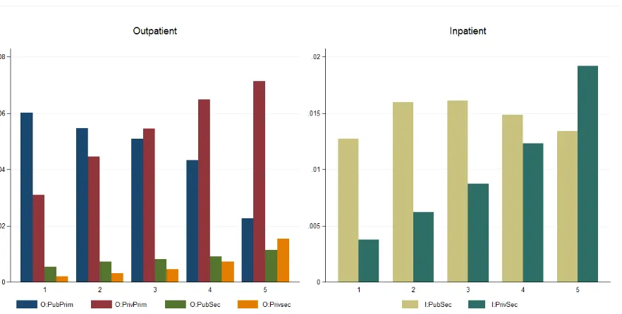
Figure 1 shows health care utilisation rates of various types of care by wealth quintiles. The utilisation rate of outpatient treatment at public primary facilities (O:PubPrim), mainly health centers or
puskesmas, is decreasing in wealth whilst the opposite is true for outpatient treatment at private primary
facilities (O:PrivPrim), mainly doctors’ clinics. Outpatient care at secondary facilities (hospitals) also shows strong positive correlation with wealth, especially at private hospitals (O:PrivSec).For inpatient care, hospitalisation at private hospital (I:Priv) shows very strong positive correlation with wealth while hospitalisation at public hospital (I:Pub) is relatively equally spread across wealth quintiles.
Figure 1: Health care utilisation across wealth quintiles
Figure2plots a series ofconcentration curves toillustrate access inequities to various types of health
care in the overall population during 2011-2016. The concentration curves plot the cumulative distribution of each type of care as a function of the cumulative distribution of the population ranked
by its wealth. A 45-degree line represents the line of equity, in which health care utilisation is
independent of wealth. A concentration curve that lies below (above) the 45-degree line indicates a
situation in which the use of that particular health service is more concentrated among the wealthier
(poorer) of the population or “pro-rich” (“pro-poor”). The further is the concentration curve from the
45-degree line, the greater is the extent of the access inequity. Figure 2 reveals that only access to
outpatient care at puskesmasis pro-poor whilst access to other types of health care is pro-rich. The
greatest inequities are observed for services at private hospitals.
Figure 2: The concentration curves of various types of health care
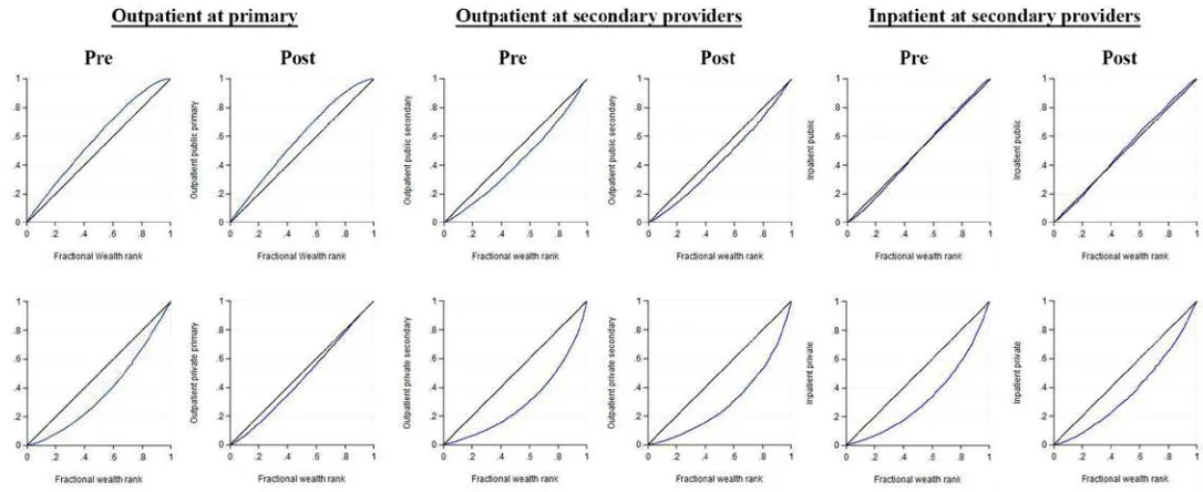
Figure 3 shows the concentration curves before (pre-) and after (post-) the introduction of JKN.We define 2011-2013 as the pre-JKN period and 2015-2016 as the post-JKN period. Year 2014 is excluded because SUSENAS 2014 was fielded at four points in 2014: March, June, September and December, which means that the bulk of inpatient utilisationsfor households interviewed in March and June would include utilisation in the second half of 2013, before JKN was introduced. We observe that, post-JKN, almost all concentration curves that lie under the line of equity have moved closer to the line of equity, indicating that, access to these services have become more pro-poor than before. The shift is particularly apparent for outpatient care at private clinics. Outpatient care at puskesmashas remained pro-poor.
Figure 3: Concentration indices of various types of health care pre- and post-JKN
Note: y-axis plots the cumulative density of a health care use by individuals ranked from the least wealthy to the wealthiest, weighted by population frequency weight. Pre-JKN uses data from pooled SUSENAS 2011-2013 and post-JKN uses data from pooled SUSENAS 2015-2016. The wealth quintiles are computed by year at the household-level, using population frequency weight, before creating the pooled data. The concentration index (CI) for each year and each type of health care is computed using population frequency weight. All concentration indices are statistically significant at any conventional significance level.
Table 1, under the heading of ‘Overall’, summarises the pictures in Figure 3 through the change in CIs pre-and post-JKN. The CI measures the distance between the line of equity to the concentration curve. Pre-JKN, outpatient care at puskesmas has a negative CI, as it is pro-poor. Outpatient care at public hospitals and services at privatefacilities have positive CIs, as they are pro-rich. Inpatient care at public hospitals has a CI that is very close to 0. Post-JKN, the CIs for outpatient care at puskesmas and private
accepting JKN patients. Access to inpatient care at public hospitals turns slightly pro-poor. Some of these improvements support JKN as a pro-poor program that is positively associated with a reduction
in wealth-related inequity in access to health care. The rest of Table 1 reproduces the results for urban
and rural samples. It reveals that the CI for inpatient care at public hospitals has different signsin urban
and rural areas: the CI is negative in urban areas (access is pro-poor) and positive in rural areas (access
is pro-rich), giving an aggregate picture of no inequity (CI close to 0). Except for servicesat puskesmas,
the fall in CIs are found larger in urban than in rural areas.
Table 1: Concentration indices of various types of health care pre- and post-JKN
Overall Urban Rural
Pre Post Pre Post Pre Post
O: public primary -0.176 -0.176 -0.261 -0.256 -0.127 -0.133 (t-statistics) (-114.1) (-97.55) (-107.3) (-91.56) (-64.14) (-56.47)
O: private primary 0.264 0.071 0.135 0.017 0.277 0.142
(t-statistics) (160.5) (50.98) (61.03) (8.20) (104.4) (76.35)
O: public secondary 0.153 0.124 0.063 0.045 0.116 0.119
(t-statistics) (40.88) (33.15) (12.29) (8.57) (20.25) (21.33)
O: private secondary 0.407 0.407 0.326 0.339 0.280 0.285
(t-statistics) (97.59) (98.62) (61.69) (64.78) (36.34) (37.53)
I: public 0.009 -0.018 -0.076 -0.085 0.083 0.056
(t-statistics) (3.02) (-6.43) (-16.87) (-19.71) (21.24) (15.26)
I: private 0.353 0.268 0.278 0.199 0.301 0.256
(t-statistics) (94.31) (87.21) (56.06) (47.32) (48.55) (53.63) Note: ‘O’ and ‘I’ denote outpatient and inpatient care, respectively. Pre-JKN pooled data from SUSENAS 2011-2013 and Post-JKN pooled data from SUSENAS 2015-2016. The concentration index for each type of health care is computed using population frequency weight. All concentration indices are statistically significant at any conventional significance level.
Table 2 showshow various determinants contribute to access inequities (Equation (3)). For conciseness,
we report only the contribution of eachdeterminant’s inequity to the access inequity and keep the full
results, including the elasticity and concentration index of each determinant in Appendix. For outpatient
care at puskesmas, we find that the biggest contributors to its pro-poor access inboth pre-and post-JKN
periods are pro-poor health care needs, driven by age factor, wealth, households’ earning ability
indicators (age and education of household head), distribution PBI and availability of maternal health
facilities.For wealth and households’ earning ability indicators,their contributions are pro-poorbecause
these economic variables are positively related with wealth (CI>0) but well-off individuals are less
likely to go to puskemasto obtain health care (elasticity<0). Counteracting the pro-poor factors arepro
-rich remoteness, local village development unobserved factors. The latter may capture supply disadvantages such as overcrowding, forcing prioritisation of patients that disfavours the poor.
12
Table 2: Contributions of various determinants to access inequity pre- and post-JKN
O: public primary O: private primary O: public secondary O: private secondary I: public I: private
Pre Post Pre Post Pre Post Pre Post Pre Post Pre Post
Health needs
Age -0.1790 -0.2082 -0.0974 -0.2165 0.0151 0.0529 -0.1274 -0.1152 -0.0848 -0.1704 -0.1726 -0.3584
Male -0.0015 -0.0013 0.0000 -0.0009 -0.0023 -0.0019 -0.0030 -0.0008 -0.0046 -0.0071 -0.0062 -0.0094
# sick days -0.0171 -0.0159 -0.0211 -0.0179 -0.0421 -0.0446 -0.0314 -0.0338 -0.0271 -0.0226 -0.0222 -0.0166 Non-health
Age of household head -0.0769 -0.0968 -0.0407 -0.1021 0.0928 0.1204 0.0318 0.0579 0.0404 0.0217 0.0573 0.0608 Male household head -0.0037 -0.0021 -0.0055 -0.0017 -0.0034 -0.0038 -0.0075 -0.0078 -0.0037 -0.0011 -0.0073 -0.0029
Wealth quintile -0.2953 -0.3541 0.5764 0.2617 0.3323 0.2454 0.6517 0.5704 0.2500 0.0862 0.7370 0.5267
Education of household head -0.0433 -0.0353 0.0131 -0.0197 0.1148 0.0722 0.1212 0.1122 0.0316 -0.0073 0.0841 0.0143
Married 0.0017 0.0014 0.0017 0.0023 0.0001 -0.0005 0.0023 0.0027 0.0035 0.0056 0.0056 0.0117
Divorced/separated -0.0001 -0.0001 -0.0001 -0.0001 0.0002 0.0001 -0.0001 0.0000 -0.0003 -0.0004 -0.0004 -0.0007
Widowed -0.0010 -0.0006 -0.0008 -0.0006 0.0005 0.0004 -0.0002 0.0007 -0.0015 -0.0013 -0.0020 -0.0024
Insurance
SHI non PBI -0.0129 0.0122 0.0149 -0.0009 0.0311 0.1116 0.0290 0.0713 0.0147 0.0740 0.0307 0.0494
PBI -0.0459 -0.0662 0.0100 0.0144 -0.0431 -0.0568 -0.0015 0.0079 -0.0648 -0.0575 -0.0047 0.0010
Private -0.0043 -0.0047 0.0032 0.0010 -0.0033 0.0009 0.0210 0.0510 -0.0001 -0.0007 0.0163 0.0198
SHI/PBI and private 0.0042 -0.0008 0.0021 0.0004 0.0050 0.0010 0.0107 0.0107 0.0059 0.0004 0.0068 0.0058 Geo
Rural 0.0324 0.0291 0.0683 -0.0179 0.0969 0.0666 0.0248 0.0211 0.0472 0.0287 0.0206 0.0089
Village development index 0.0567 0.0883 -0.0125 -0.0689 0.0158 -0.0156 0.1459 0.1129 -0.0914 -0.0942 0.0590 0.0494 Health infrastructure
Primary 0.0015 0.0044 -0.0017 0.0012 -0.0038 -0.0051 -0.0048 0.0010 0.0045 0.0029 -0.0045 -0.0010
Secondary 0.0148 -0.0009 0.0083 0.0171 0.0083 0.0056 -0.0029 0.0131 0.0243 0.0073 0.0243 0.0288
Maternal -0.0134 -0.0073 -0.0020 0.0043 -0.0057 -0.0039 -0.0163 -0.0224 0.0106 0.0142 -0.0041 -0.0127
13
Other unobserved 0.4099 0.4853 -0.2491 0.2175 -0.4423 -0.4101 -0.4192 -0.4324 -0.1366 0.1090 -0.4500 -0.0972
Total -0.1756 -0.1759 0.2643 0.0713 0.1527 0.1242 0.4065 0.4072 0.0089 -0.0181 0.3534 0.2683
HI (Total – Health needs) 0.0220 0.0495 0.3829 0.3067 0.1820 0.1178 0.5683 0.5570 0.1253 0.1819 0.5543 0.6526
Note: ‘O’ and ‘I’ denote outpatient and inpatient care, respectively. Pre-JKN pooled data from SUSENAS 2011-2013 and Post-JKN pooled data from SUSENAS 2015-2016. The sample size for pre-and post-JKN period is 3,332,383 and 2,207,463, respectively. For age and sex, their marginal effects are computed taking into account higher power
For outpatient care at private doctors’ clinics, the bulk of its pro-rich access in both pre-and post-JKN periodsis caused by pro-rich wealth, PBI and availability of hospitals.The contribution of PBI is pro
-rich because PBI is negatively correlated with wealth (CI<0) and PBI beneficiaries have lower likelihood to seek care at private clinics (elasticity<0). In the pre-JKN period, remoteness and SHI also
has large pro-rich contribution. On the other hand, health care needsand local village development are
pro-poor in both periods. Unobserved factors were pro-poor pre-JKN but turned pro-rich post-JKN.
This may reflect depletion of excess capacity or other supply advantages in areas where rich people use
many health services (e.g., greater health technology investments, greater price competition, etc), which formerly allow extension of services to poorer patients.
Pro-rich access to outpatient cares at public and private hospitals are driven by pro-rich wealth,
households’ earning ability, SHI and remoteness. For outpatient care at private hospitals, pro-rich
private health insurance membership and village development also explain the pro-rich access.
Unobserved factors are pro-poorin both periods.
For inpatient care, the contributors to its pro-rich access in both public and private hospitals are pro
-rich wealth, households’ earning ability, SHI, remoteness and availability of hospitals. At public
hospitals, the counteracting factors are pro-poor health care needs, PBI and local economic
development.3The last two results are interesting as they may suggest that some form of targeted health
insurance like PBI and policies that stimulate local economic growth can be used to reduce
wealth-related inequity in access to inpatient care at public hospitals. Unobserved factors are pro-poor pre-JKN
and pro-rich post-JKN. At private hospitals, village development and private health insurance add to
pro-rich access. Meanwhile, unobservables are pro-poorin both periods.
The last row of Table 2 reports the horizontal index (HI) of each type of health care. Since distribution of health care needs is pro-poor (the poor tend to be more prone to illness), HIs tend to be bigger than
CIs, indicating that access inequities are more pro-rich when health care needs are taken into account.
That is, for a given health care need, the rich makes greater use of formal health servicesthan the poor.4
For outpatient care at puskesmas, we find that HI is positive suggesting that the pro-poorness of health
care needs explains the bulk of its pro-poor access.
Table 3 showschanges in the roles of access determinants pre-and post-JKN, and how far these changes
were due to changes in elasticities rather than changes in inequities(Equation (6)). We find that in most
cases, it is the changing elasticities (Δelas)rather than changing inequities (Δcon)that accounts for the
3The measure for this is derived from the first component of a principal component analysis with inputs including
the availability of a post office, modern market, banks, strong telephone signal, asphalt road, garbage collection system, piped water, etc in the village. Villages are then ranked based on their first component, then assigned to quintiles.
4HI however does not capture the tendency for the poor to have lower health knowledge and awareness to seek
bulk of the change in access inequities. In particular, there are big drops in the elasticities (propensity
of use and/or mean) of wealth and households’ earning ability indicators as they become less pro-rich
or more pro-poor. Except for access to puskesmas, there are also reductions in the elasticities of
remoteness and local village development. These effects make access more pro-poor. An exception
relates to health care needs. The correlation between health care needs, mainly age, and wealth (CI) is
stronger post-JKN, resulting in ∆con that is pro-poor for most services, as they are less likely to be used
by older individuals. For SHI,Δcon and Δelas of SHI have counteracting effects with the latter being
the dominant effect. Δcon<0 indicates that the distribution of SHI becomesmore pro-poor post-JKN.
Since we have separated out PBI from SHI, this effect may capture enrolments by informal sector
workersandemployers of private companies, which previously opt-out from state insurance. However,
the total effect is still contributing topro-rich access gap because propensity to seek care SHI members,
who arerelatively well-off (CI>0), have also increased considerably (Δelas>0). Utilisation of doctors’
clinics is an exception, as SHI members are less likely to visit this facility post-JKN. For PBI, Δelas<0
at public facilities and Δelas>0 at private facilities. Because PBIhas a negative CI (i.e., PBI is negatively
related to wealth), Δelas>0 suggests that PBI beneficiaries are increasingly less likely to obtain
outpatient care at private facilities.This result may indicatethat, unlike SHI members who are accessing
various health services, PBI beneficiaries may still be restricted in access to private facilities. With
regards to the changing rolesof unobserved factors, they are mostly pro-rich, which is not inconsistent
with the story that they capture supply-side advantages or disadvantages; asthe demand for health care
by the poorer expands, supply advantages are spread more thinly whilst supply disadvantages force
16
Table 3: Oaxaca- Blinder type decomposition for change in access inequity pre- and post-JKN
O: public primary O: private primary O: public secondary O: private secondary I: public I: private
Δcon Δelas Δcon Δelas Δcon Δelas Δcon Δelas Δcon Δelas Δcon Δelas
Health needs
Age -0.0665 0.0373 -0.0692 -0.0499 0.0169 0.0209 -0.0368 0.0490 -0.0544 -0.0312 -0.1145 -0.0712
Male -0.0003 0.0006 -0.0002 -0.0007 -0.0005 0.0009 -0.0002 0.0024 -0.0017 -0.0008 -0.0023 -0.0009 # sick days 0.0026 -0.0015 0.0030 0.0002 0.0074 -0.0099 0.0056 -0.0080 0.0037 0.0008 0.0027 0.0029 Non health
Age of household head -0.0231 0.0032 -0.0243 -0.0371 0.0287 -0.0011 0.0138 0.0123 0.0052 -0.0239 0.0145 -0.0110 Male household head 0.0003 0.0014 0.0002 0.0035 0.0005 -0.0010 0.0011 -0.0014 0.0001 0.0025 0.0004 0.0040 Wealth quantile -0.0004 -0.0583 0.0003 -0.3150 0.0003 -0.0872 0.0007 -0.0820 0.0001 -0.1639 0.0006 -0.2109 Educ of household head 0.0026 0.0053 0.0015 -0.0342 -0.0054 -0.0372 -0.0084 -0.0006 0.0005 -0.0394 -0.0011 -0.0687 Married 0.0005 -0.0008 0.0009 -0.0003 -0.0002 -0.0004 0.0010 -0.0007 0.0022 -0.0001 0.0046 0.0015 Divorced/separated 0.0000 0.0000 0.0000 0.0000 0.0000 -0.0002 0.0000 0.0000 0.0000 -0.0001 0.0000 -0.0003
Widowed 0.0001 0.0002 0.0001 0.0000 -0.0001 0.0000 -0.0001 0.0010 0.0003 -0.0001 0.0005 -0.0010
Insurance
SHI (non PBI) -0.0069 0.0321 0.0005 -0.0163 -0.0636 0.1440 -0.0406 0.0829 -0.0422 0.1016 -0.0282 0.0468
PBI 0.0091 -0.0294 -0.0020 0.0063 0.0078 -0.0215 -0.0011 0.0105 0.0079 -0.0006 -0.0001 0.0059
Private -0.0021 0.0018 0.0004 -0.0027 0.0004 0.0038 0.0234 0.0066 -0.0003 -0.0002 0.0091 -0.0055
SHI/PBI and private -0.0005 -0.0044 0.0003 -0.0020 0.0006 -0.0046 0.0067 -0.0067 0.0003 -0.0058 0.0036 -0.0047 Geo
Rural -0.0029 -0.0004 0.0018 -0.0879 -0.0067 -0.0236 -0.0021 -0.0016 -0.0029 -0.0156 -0.0009 -0.0107 Village dev index -0.0035 0.0351 0.0027 -0.0591 0.0006 -0.0320 -0.0044 -0.0286 0.0037 -0.0064 -0.0019 -0.0076 Health infrastructure
Primary -0.0007 0.0035 -0.0002 0.0031 0.0008 -0.0020 -0.0002 0.0060 -0.0005 -0.0011 0.0002 0.0033 Secondary 0.0002 -0.0159 -0.0032 0.0120 -0.0010 -0.0016 -0.0024 0.0184 -0.0014 -0.0155 -0.0053 0.0099
Maternal 0.0010 0.0052 -0.0006 0.0070 0.0005 0.0012 0.0030 -0.0091 -0.0019 0.0055 0.0017 -0.0104
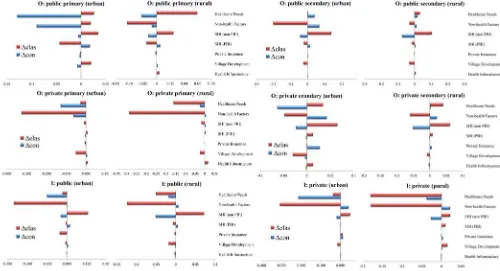
As there are likely to be significant differences in urban and rural areas (Table 1), we repeat the above decomposition exercises for urban and rural sample, separately. Figures 5-6 summarise the results. Figure 5 shows the sources of access inequities in each area pre- and post-JKN. Most observables variables contribute in the same direction to access inequities in rural and urban areas. However, health insurance variableshave larger roles in urban areas. Recall that inpatient care at public hospitals is pro-poor in urban areas but pro-rich in rural areas (Table 2). Figure 4 shows that the pro-rich access in rural areas is due to strong pro-rich non-health (economic) factors that are unmatched by pro-poor health needs and PBI distribution. Post-JKN, there are also pro-rich push to access to rural public hospital beds by unobservables.
Figure 4: Contributions of various determinants to access inequity pre- and post-JKN by remoteness
Note: each section of each bar shows the contribution of a given (group of) determinant on access inequity to that particular health service according to Equation (3). Pre-JKN uses data from pooled SUSENAS 2011-2013 and post-JKN uses data from pooled SUSENAS 2015-2016.
Figure 5 shows that, as with the overall sample, in both areas, most changes are driven by changing elasticities, more so than by changing inequities of access determinants. The large pro-poor push due to falling ∆con of health care needs we saw earlier in the overall sample occurs in urban areas. This is driven by a considerable increase in the CI of age in urban areas while older individuals are less likely to visit health facilities than the young. Differently, in rural areas, pro-poor ∆elas of health care needs is dominant in reducing pro-rich access to private clinics and inpatient care. Except at urban puskesmas,
on other hand, the falling contribution of non-health factors is due to pro-poor ∆con. CIs of non-health factors in urban areas increase significantly resulting in large pro-poor Δconbecause the better-off in these areas are very unlikely to visit puskesmas (large negative elasticity). More pro-poor distribution
of SHI (∆con<0) has larger counteracting effect to ∆elas in rural areas. We also observe urban-rural differences in the contributionsof health infrastructure to access inequity to outpatient care at private hospitals and village development to access inequity at private hospitals.
Figure 5: Oaxaca- Blinder type decomposition for change in access inequity pre- and post-JKN by remoteness
Note: each bar shows the extent of the change in access inequity that is due to changing elasticity and changing inequity of a given determinant according to Equation (6). Pre-JKN uses data from pooled SUSENAS 2011-2013 and post-JKN uses data from pooled SUSENAS 2015-2016.
As insurance is our key variables, we further investigate whether their changing elasticities post-JKN
are driven by a real change in the propensity of health care use (∆beta), rather than the implication of a
tend to be used by SHI members. On the other hand, for PBI that is always more pro-poor than utilisation, ∆mean will be positive for services that are less likely to be used by PBI beneficiaries.∆beta reflects the relationship between insurance and utilisation. For SHI, ∆beta>0 indicates that SHI members are increasingly more likely to use that particular health care services than before, whilst for PBI, ∆beta>0 indicates that PBI beneficiaries are increasingly less to use that health care services than before.
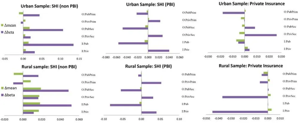
Figure 6 provides a graphical representation of the results. In both urban and rural areas,∆beta of SHI is positive and dominant, except for outpatient care at doctors’ clinics, indicating that utilisation has become more sensitive to SHI status post-JKN. For PBI, inboth areas, almost all ∆elas are driven by ∆mean: propensity to use public care increases whilst propensity to use private care falls. For private insurance, in urban areas, falling insurance rate has pro-poor contributions to most care, while ∆beta is also pro-poor for access to puskesmas services and public beds. In rural areas, ∆beta is pro-poorfor all primary care and services at private hospitals, suggesting that privately insured individuals are increasingly less likely to use these services. A possible explanation for this may be that the smaller private insurance pool (from 4.6% of the sample pre-JKN to 0.5% post-JKN) consists of relatively healthy, wealthy individuals who need less medical attention.
Figure 6: Sources of changing elasticities of access determinants pre- and post-JKN by remoteness
5. Conclusion
This paper has examined the extent of access inequities of various health care in Indonesia during
2011-2016. Access to outpatient care at public primary facilities, mainly puskesmas, is pro-poor, while access
to most other types of health care is pro-rich. Access to inpatient care at public hospitals is nearly universal at the national level but this masks significant variation according to geographical location. Inpatient care at public hospitals in urban areas is pro-poor whilst it is pro-rich in rural areas. Pro-rich access is driven by pro-rich non-health factors, mainly households’ economic status, geographical
factorsand non-targeted health insurance (SHI). Counteracting these factors are pro-poor health care
needs. Inequities in local village development, health infrastructure, targeted health insurance (PBI) and
unobservable factors have different contributions to access inequity depending on the type of care.
Village development has pro-rich contributions on access to puskesmas services, while health
infrastructure has pro-rich contributions to inpatient care, especially in rural areas. On the other hand,
pro-poor PBI has pro-poor contributions on access to all health services at public facilities, and
unobservables have pro-poor contributions on access to outpatient care at hospitals and private hospital
beds.
With the introduction of JKN in 2014, which increases the aggregate health insurance rate, access to
most health care services is still pro-rich but they become less pro-rich ormore pro-poorthan before.
The biggest changes are observed for access to outpatient care at private clinics and inpatient care at
private hospitals. Urban areas see bigger changes. The primary driver of thispro-poor movement is
much weaker association between households’ economic status and utilisation. This effect is consistent with the rationale of insurance as a consumption-smoothing mechanism; that is, the expansion of health
insurance due to JKN lowers the incidence of a household having to pay very expensive medical bill in
the event of an adverse health shock. Some of this pro-poor movement however is being counteracted
by increasing propensity of utilisation by SHI members, except for services at private clinics. While
SHI’s distribution is more pro-poor post-JKN, SHI is still positively related to wealthso an increased
utilisation by SHI members has pro-rich effect. For PBI, we find that PBI beneficiaries havehigher
propensity to use public facilities but lower propensity to use private facilities. We also observe changing roles of unobservable factors in explaining access inequity of private clinics and public hospital beds. Pre-JKN, unobservables have pro-poor contributions to access to these services but they turn pro-rich post-JKN.
Even with the introduction of JKN, there are still critical challenges in the Indonesian health care system
that prevent it from being pro-poor, such lack of supply-side readiness, limited public investments in health infrastructure, human resource constraints and pharmaceutical maldistribution to rural and
have lower health knowledge and awareness to seek medical care. Furthermore, while JKN may have
covered most of formal sector workers, it has yet to reach more of those in informal sector.
Our results have several policy implications. First, while accesses to most health services in Indonesia
are still favouring the wealthier, JKN has helped to reduce the size of the access gaps. Hence, as we move towards universal coverage, we may expect further reduction in access gap. Second, there may be wider scope to further improve access inequity in rural areas. Hitherto, bigger reductions in access gaps were observed in urban areas. Some policies may need to be specifically tailored to be more
effective in rural areas. Third, policymakers need to ensure that distribution of targeted program (PBI)
is pro-poor, since we find evidence thatitbecomes less pro-poor post-JKN. Fourth, we find noevidence
that the distribution of health infrastructure has become more equal post-JKN. To serve more patients,
improvements need totake place in both the physical quantity of health facilitiesand the adequacy of
References
Bago d’Uva T, Jones AM, Van Doorslaer E. 2009. Measurement of horizontal inequity in health care
utilisation using European panel data. Journal of Health Economics 28: 280–289.
Bonfrer I, Van De Poel E, Grimm M, Van Doorslaer E. 2014. Does the distribution of healthcare
utilization match needs in Africa? Health Policy and Planning 29: 921–937.
Doorslaer EV, Koolman X, Jones AM. 2004. Explaining income-related inequalities in doctor
utilisation in Europe. Health Economics 13: 629–647.
Elwell-Sutton TM, Jiang CQ, Zhang WS, et al. 2013. Inequality and inequity in access to health care and treatment for chronic conditions in China: the Guangzhou Biobank Cohort Study. Health Policy
and Planning 28: 467–479.
Habicht, J. and Kunst, A.E. (2005). Social Inequalities in Health Care Services Utilization After Eight Years of Health Care Reforms: A Cross-sectional Study of Estonia, 1999. Social Science & Medicine
60: 777–787.
Hotchkiss DR, Godha D, Do M. 2014. Expansion in the private sector provision of institutional delivery services and horizontal equity: evidence from Nepal and Bangladesh. Health Policy Planning 29(Suppl
1): i12–i19.
Johar, M., Jones, G., Keane, M., Savage, E., Stavrunova, O. 2013. Discrimination In A Universal Health Care System: Explaining Socioeconomic Waiting Time Gaps. Journal of Health Economics 32(1): 181-194.
Kakwani N, Wagstaff A, Van Doorslaer E. 1997. Socioeconomic inequalities in health: measurement,
computation, and statistical inference. Journal of Econometrics 77: 87–103.
Koolman X, Van Doorslaer E. 2004. On the interpretation of a concentration index of inequality. Health
Economics 13: 649–656.
Leung GM, Tin KY, O’Donnell O. 2009. Redistribution or horizontal equity in Hong Kong’s mixed
public–private health system: a policy conundrum. Health Economics 18: 37–54.
Liu GG, Zhao Z, Cai R., Yamada T, Yamada T. 2002. Equity in health care access to: assessing the
urban health insurance reform in China. Social Science & Medicine 55: 1779–1794.
Lu JR, Leung GM, Kwon S, Tin KYK, Van Doorslaer E, O’Donnell O. 2007. Horizontal equity in health care utilization evidence from three high-income Asian economies. Social Science & Medicine
64: 199–212.
O’Donnell O, Van Doorsslaer E, Wagstaff A, Lindelow M. 2008. Analyzing Health Equity Using Household Survey Data: A Guide to Techniques and Their Implementation. World Bank Publications. Paredes, K.P.P., 2016. Inequality in the use of maternal and child health services in the Philippines: do pro-poor health policies result in more equitable use of services?.International Journal for Equity in
Quayyum, Z., Khan, M.N.U., Quayyum, T., Nasreen, H.E., Chowdhury, M. and Ensor, T., 2013. “Can
community level interventions have an impact on equity and utilization of maternal health care”–
Evidence from rural Bangladesh. International journal for equity in health, 12(1), p.22.
Saito, E., Gilmour, S., Yoneoka, D., Gautam, G.S., Rahman, M.M., Shrestha, P.K. and Shibuya, K., 2016. Inequality and inequity in healthcare utilization in urban Nepal: a cross-sectional observational study. Health policy and planning, 31(7), pp.817-824.
UNICEF. 2012. Issue Briefs: Maternal and child health. Available from
https://www.unicef.org/indonesia/A5-_E_Issue_Brief_Maternal_REV.pdf
Van Doorslaer E, Masseria C. 2004. Income-Related Inequality in the Use of Medical Care in 21 OECD Countries. OECD.
Van Doorslaer E, Wagstaff A, Van Der Burg H, et al. 2000. Equity in the deliveryof health care in Europe and the US. Journal of Health Economics 19: 553.
Veugelers, P.J. and Yip, A.M., 2003. Socioeconomic disparities in health care use: Does universal coverage reduce inequalities in health? Journal of Epidemiology and Community Health, 57(6), pp.424-428.
Wagstaff A, Van Doorslaer E. 2000. Measuring and testing for inequity in the delivery of health care.
Journal of Human Resources 35: 716–733.
Wagstaff, A., van Doorslaer, E., Watanabe. N. 2003. On Decomposing the Causes of Health Sector Inequalities, with an Application to Malnutrition Inequalities in Vietnam. Journal of Econometrics
112(1): 219–27.
24
APPENDIX Detailed results
1. ALLSAMPLE: Detailed results
Mean Concentration Index O: Public PrimaryCoefficients O: Public PrimaryElasticity O: Private PrimaryCoefficients O: Private PrimaryElasticity
Pre Post Pre Post Pre Post Pre Post Pre Post Pre Post
Health needs
Age 27.8926 28.3973 0.1909 0.2805 -0.0069 -0.0059 -0.9376 -0.7422 -0.0040 -0.0108 -0.5105 -0.7719
Male 0.5063 0.5062 -0.0100 -0.0132 0.0030 0.0012 0.1503 0.0951 0.0002 0.0037 -0.0007 0.0675
# sick days 0.7325 0.8398 -0.0853 -0.0732 0.0120 0.0126 0.2001 0.2178 0.0129 0.0246 0.2476 0.2453
Non-health
Age of household head 47.116 47.741 0.2257 0.2963 -0.0003 -0.0003 -0.3408 -0.3266 -0.0001 -0.0006 -0.1802 -0.3446 Male household head 0.9121 0.9078 0.0367 0.0323 -0.0049 -0.0035 -0.1016 -0.0645 -0.0062 -0.0049 -0.1490 -0.0528
Wealth quantile 3.1205 3.1055 0.7959 0.7969 -0.0052 -0.0070 -0.3710 -0.4443 0.0088 0.0089 0.7242 0.3285
Education of household head 2.1247 2.2020 0.2598 0.2417 -0.0034 -0.0032 -0.1665 -0.1459 0.0009 -0.0031 0.0503 -0.0815
Married 0.4653 0.4656 0.0115 0.0189 0.0138 0.0076 0.1458 0.0731 0.0123 0.0220 0.1500 0.1218
Divorced/separated 0.0116 0.0127 -0.0671 -0.0676 0.0055 0.0055 0.0014 0.0015 0.0068 0.0124 0.0021 0.0019
Widowed 0.0379 0.0378 -0.0722 -0.0591 0.0153 0.0133 0.0132 0.0104 0.0109 0.0231 0.0108 0.0104
Insurance
SHI (non PBI) 0.1266 0.2277 0.6108 0.3890 -0.0074 0.0067 -0.0212 0.0313 0.0073 -0.0008 0.0244 -0.0022
PBI 0.2652 0.2861 -0.4157 -0.3655 0.0183 0.0308 0.1105 0.1812 -0.0035 -0.0116 -0.0241 -0.0393
Private 0.0450 0.0158 0.3821 0.7060 -0.0111 -0.0204 -0.0113 -0.0066 0.0071 0.0072 0.0085 0.0014
SHI/PBI and private 0.0222 0.0035 0.2726 0.7287 0.0303 -0.0145 0.0153 -0.0010 0.0132 0.0134 0.0077 0.0006 Geo
Rural 0.4951 0.4870 -0.5976 -0.5428 -0.0048 -0.0053 -0.0542 -0.0535 -0.0088 0.0057 -0.1142 0.0329
Village development index 1.3803 1.8461 0.2001 0.1925 0.0090 0.0121 0.2832 0.4585 -0.0017 -0.0163 -0.0624 -0.3577 Health infrastructure
Primary 0.8143 0.8428 0.0347 0.0301 0.0023 0.0084 0.0433 0.1450 -0.0023 0.0039 -0.0494 0.0387
Secondary 0.8064 0.8350 0.0537 0.0453 0.0151 -0.0012 0.2760 -0.0202 0.0073 0.0380 0.1537 0.3772
ALL SAMPLE: Detailed results (continued)
O: Public Secondary O: Public Secondary O: Private Secondary O: Private Secondary
Coefficients Elasticity Coefficients Elasticity
Pre Post Pre Post Pre Post Pre Post
Health needs
Age -0.0006 -0.0006 0.0792 0.1887 -0.0009 -0.0007 -0.6672 -0.4106 Male 0.0016 0.0014 0.2332 0.1449 0.0017 -0.0002 0.3002 -0.0008 # sick days 0.0049 0.0079 0.4942 0.6103 0.0029 0.0049 0.3682 0.4622
Non-health
Age of household head 0.0001 0.0001 0.4113 0.4063 0.0000 0.0000 0.1408 0.1953 Male household head -0.0007 -0.0014 -0.0918 -0.1184 -0.0013 -0.0024 -0.2042 -0.2427 Wealth quantile 0.0010 0.0011 0.4176 0.3080 0.0015 0.0021 0.8188 0.7157 Education of household
head 0.0015 0.0015 0.4417 0.2986 0.0013 0.0019 0.4666 0.4642 Married 0.0001 -0.0006 0.0072 -0.0254 0.0025 0.0027 0.1989 0.1405 Divorced/separated -0.0021 -0.0007 -0.0033 -0.0008 0.0004 0.0005 0.0009 0.0007 Widowed -0.0013 -0.0021 -0.0067 -0.0072 0.0004 -0.0026 0.0024 -0.0111
Insurance
SHI (non PBI) 0.0029 0.0137 0.0510 0.2868 0.0022 0.0072 0.0475 0.1832 PBI 0.0028 0.0059 0.1037 0.1553 0.0001 -0.0007 0.0035 -0.0216 Private -0.0014 0.0009 -0.0085 0.0013 0.0070 0.0406 0.0548 0.0722 SHI/PBI and private 0.0059 0.0041 0.0183 0.0013 0.0102 0.0372 0.0393 0.0146
Geo
Rural -0.0024 -0.0027 -0.1621 -0.1226 -0.0005 -0.0007 -0.0415 -0.0388 Village development
index 0.0004 -0.0005 0.0788 -0.0812 0.0031 0.0028 0.7293 0.5865
Health infrastructure
ALL SAMPLE: Detailed results (continued)
I: Public I: Public I: Private I: Private Coefficients Elasticity Coefficients Elasticity
Pre Post Pre Post Pre Post Pre Post
Health needs
Age -0.0015 -0.0007 -0.4441 -0.6074 -0.0013 -0.0033 -0.9043 -1.2776
Male 0.0044 0.0084 0.4589 0.5357 0.0036 0.0082 0.6173 0.7118
# sick days 0.0050 0.0072 0.3174 0.3084 0.0025 0.0044 0.5159 0.2265
Non-health
Age of household head 0.0000 0.0000 0.1791 0.0732 0.0000 0.0001 0.2539 0.2052 Male household head -0.0013 -0.0007 -0.1018 -0.0331 -0.0016 -0.0016 -0.1985 -0.0907 Wealth quantile 0.0012 0.0007 0.3141 0.1082 0.0021 0.0034 0.9259 0.6609 Education of household
head 0.0007 -0.0003 0.1217 -0.0301 0.0011 0.0004 0.3237 0.0592 Married 0.0075 0.0124 0.3018 0.2951 0.0074 0.0215 0.4836 0.6185 Divorced/separated 0.0041 0.0085 0.0041 0.0055 0.0036 0.0131 0.0059 0.0103 Widowed 0.0065 0.0116 0.0212 0.0224 0.0051 0.0172 0.0272 0.0404
Insurance
SHI (non PBI) 0.0022 0.0163 0.0241 0.1904 0.0028 0.0090 0.0503 0.1269
PBI 0.0068 0.0107 0.1559 0.1572 0.0003 -0.0002 0.0114 -0.0027
Private -0.0001 -0.0012 -0.0004 -0.0009 0.0068 0.0287 0.0425 0.0281 SHI/PBI and private 0.0114 0.0033 0.0218 0.0006 0.0081 0.0366 0.0250 0.0079
Geo
Rural -0.0019 -0.0021 -0.0790 -0.0529 -0.0005 -0.0005 -0.0344 -0.0165 Village development index -0.0039 -0.0052 -0.4570 -0.4893 0.0015 0.0022 0.2947 0.2566
Health infrastructure
27
2. URBAN:Contributions of various determinants to access inequity pre-and post-JKN
O: Public Primary O: Private primary O: Public secondary O: Private secondary I: Public I: Private
Pre Post Pre Post Pre Post Pre Post Pre Post Pre Post
Health needs
Age -0.1225 -0.2255 -0.0703 -0.2240 0.0223 0.0708 -0.0822 -0.1114 -0.0518 -0.1743 -0.1199 -0.3697
Male -0.0035 -0.0016 -0.0001 -0.0015 -0.0047 -0.0020 -0.0056 0.0019 -0.0095 -0.0111 -0.0113 -0.0155
# sick days -0.0159 -0.0173 -0.0207 -0.0210 -0.0414 -0.0498 -0.0310 -0.0380 -0.0276 -0.0269 -0.0219 -0.0186
Non-health
Age of household head -0.0543 -0.1378 -0.0330 -0.1354 0.0504 0.1302 0.0111 0.0511 0.0144 -0.0009 0.0255 0.0264 Male household head -0.0080 -0.0027 -0.0109 -0.0020 -0.0059 -0.0071 -0.0151 -0.0175 -0.0063 -0.0008 -0.0176 -0.0061 Wealth quintile -0.5202 -0.5360 0.4838 0.2211 0.2809 0.0926 0.6097 0.5671 0.1504 -0.0625 0.6797 0.4898 Education of household
head -0.0960 -0.0723 -0.0045 -0.0372 0.1137 0.0849 0.1354 0.1325 0.0293 -0.0157 0.0998 0.0205
Married 0.0012 0.0010 0.0014 0.0020 -0.0001 -0.0008 0.0019 0.0028 0.0029 0.0055 0.0052 0.0116
Divorced/separated -0.0001 -0.0002 -0.0003 -0.0003 0.0005 0.0002 -0.0002 -0.0002 -0.0004 -0.0007 -0.0008 -0.0013
Widowed -0.0013 -0.0008 -0.0013 -0.0007 0.0008 0.0007 -0.0007 0.0006 -0.0021 -0.0015 -0.0032 -0.0032
Insurance
SHI non PBI -0.0129 0.0161 0.0141 0.0034 0.0342 0.1282 0.0275 0.0690 0.0181 0.0920 0.0284 0.0571
PBI -0.0476 -0.0733 0.0125 0.0162 -0.0466 -0.0549 -0.0026 0.0081 -0.0701 -0.0607 -0.0033 -0.0016
Private -0.0070 -0.0070 0.0045 0.0018 -0.0045 0.0029 0.0296 0.0596 0.0001 -0.0000 0.0243 0.0260
SHI/PBI and private 0.0039 -0.0008 0.0027 0.0005 0.0068 0.0019 0.0161 0.0124 0.0074 0.0008 0.0102 0.0073
Geo
Village development index 0.0612 0.0738 -0.0057 -0.0519 0.0404 0.0140 0.0710 0.0372 -0.0553 -0.0572 0.0175 0.0233
Health infrastructure
Primary -0.0006 0.0021 -0.0024 -0.0013 -0.0014 -0.0007 -0.0020 0.0046 0.0013 0.0015 -0.0050 -0.0028
Secondary 0.0054 0.0023 -0.0003 0.0068 -0.0044 -0.0043 0.0018 0.0064 0.0044 0.0009 0.0107 0.0106
Maternal -0.0030 -0.0033 0.0005 -0.0005 -0.0030 -0.0024 -0.0035 -0.0038 0.0006 0.0004 -0.0003 -0.0024
Province FE -0.0018 -0.0059 -0.0022 -0.0032 -0.0087 -0.0210 -0.0037 -0.0212 -0.0063 -0.0144 -0.0078 -0.0014
28 Other unobserved 0.5628 0.7334 -0.2334 0.2448 -0.3666 -0.3386 -0.4268 -0.4220 -0.0752 0.2404 -0.4323 -0.0392
Total -0.2600 -0.2557 0.1350 0.0175 0.0630 0.0448 0.3255 0.3392 -0.0757 -0.0853 0.2779 0.1986