Model when Occupations are
Misclassified
Paul Sullivan
a b s t r a c t
This paper develops an empirical occupational choice model that corrects for misclassification in occupational choices and measurement error in occupation-specific work experience. The model is used to estimate the extent of measurement error in occupation data and quantify the bias that results from ignoring measurement error in occupation codes when studying the determinants of occupational choices and estimating the effects of occupation-specific human capital on wages. The parameter estimates reveal that 9 percent of occupational choices in the 1979 cohort of the NLSY are misclassified. Ignoring misclassification leads to biases that affect the conclusions drawn from empirical occupational choice models.
I. Introduction
Occupational choices have been the subject of considerable research interest by economists because of their importance in shaping employment outcomes and wages over the career. Topics of study range from the analysis of job search and occupational matching (McCall 1990; Neal 1999) to studies of the determinants of wage inequality (Gould 2002) to dynamic human capital models of occupational choices (Keane and Wolpin 1997). Despite the large amount of research into occu-pational choices and evidence from validation studies such as Mellow and Sider (1983) which suggests that as many as 20 percent of one-digit occupational choices are misclassified, it is surprising that existing research has not corrected for
Paul Sullivan is a research economist at the U.S. Bureau of Labor Statistics. The author thanks John Bound, two anonymous referees, and seminar participants at Virginia, the BLS, and the Annual Meeting of the Society of Labor Economists for comments that greatly improved this paper. Financial support from a National Institute on Aging Post-Doctoral Fellowship (grant number AG00221-14) at the University of Michigan is gratefully acknowledged. The views and opinions expressed in this paper are those of the author and do not necessarily reflect the views of the Bureau of Labor Statistics. The data used in this article can be obtained beginning October 2009 through September 2012 from Paul J. Sullivan, U.S. Bureau of Labor Statistics, 2 Massachusetts Ave., NE, Suite 3105, Washington, D.C. 20212-0001 <Sullivan.Paul.Joseph@bls.gov>.
½Submitted December 2006; accepted November 2007
classification error in occupations when estimating models of occupational choice. The existence of classification error in occupations is a serious concern because in the context of a nonlinear discrete choice occupational choice model, measurement error in the dependant variable results in biased parameter estimates.
The goal of this paper is to estimate a model of occupational choices that corrects for classification error in occupation data when direct evidence on the validity of individuals’ self-reported occupations is unavailable. The approach taken in this pa-per is to specify a model of occupational choices that incorporates a parametric model of occupational misclassification. The parameters of the occupational choice model and the parameters that describe the extent of misclassification in occupation data are estimated jointly by simulated maximum likelihood. As is the case in all structural models, a limitation of this approach is that it requires the researcher to make parametric assumptions about objects in the model such as the functional form of the wage equation, the distribution of random variables that affect occupational choices, and the process by which occupations are misclassified.
The classification error literature consists of two broadly defined approaches to es-timating parametric models in the presence of classification error.1 One approach uses assumptions about the measurement error process along with auxiliary informa-tion on error rates, which typically takes the form of validainforma-tion or reinterview data, to correct for classification error. Examples of this approach to measurement error are found in work by Abowd and Zellner (1985); Chua and Fuller (1987); Poterba and Summers (1995); Magnac and Visser (1999); and Chen, Hong, and Tamer (2005). The second approach to estimating models in the presence of misclassified data cor-rects for misclassification without relying on auxiliary information by estimating parametric models of misclassification. Examples of this approach are found in Hausman, Abrevaya, and Scott-Morton (1998); Dustmann and van Soest (2001); and Li, Trivedi, and Guo (2003).
The occupational choice model developed in this paper combines features of the two existing approaches to misclassification. Instead of relying on the availability of auxiliary information that provides direct evidence on misclassified occupational choices, information about misclassification is derived from observed wages. This approach takes advantage of the fact that observed wages provide information about true occupational choices because wages vary widely across occupations. Intuitively, the occupational choices identified by the model as likely to be misclassified are the ones where the observed wage is unlikely to be observed in the reported occupation. Also, the model developed in this paper uses additional information provided by the fact that true occupational choices are strongly influenced by observable variables, such as education, to draw inferences about the extent of misclassification in the data. One methodological contribution of this work is that it develops a method of deal-ing with the problems created in panel data models when misclassification in the de-pendant variable creates measurement error in the explanatory variables in the model. Misclassification in occupation codes creates measurement error in lagged
occupational choices and occupation-specific work experience variables, so the true values of these variables are unobserved state variables. Existing research into occu-pational choices and misclassification in general has not addressed this problem.2 This work addresses the problem by using simulation methods to approximate the otherwise intractable integrals over the unobserved state variables that appear in the likelihood function.3The simulation algorithm developed in this paper is appli-cable in a wide range of settings beyond occupational choice models.
The parameter estimates provide evidence that a substantial fraction of occupa-tional choices are misclassified in the NLSY data, and suggest that ignoring misclas-sification leads to biases that affect the qualitative and quantitative conclusions drawn from estimated occupational choice models. Estimates of the transferability of human capital across occupations appear to be particularly sensitive to the false occupational transitions created by misclassification. The results also suggest that the extent of misclassification varies widely across occupations, and that observed wages provide a large amount of information about which occupational choices in the data are likely to be affected by misclassification. For example, the model pre-dicts that high wage workers who are observed as professionals are very likely to be correctly classified, but low wage workers observed as professionals are likely to be misclassified.
The remainder of the paper is organized as follows. Section II describes the data and discusses the possible sources of measurement error in occupation codes. Section III presents the model of occupational choices and misclassification and discusses how the model is estimated. Section IV presents the parameter estimates, and Section V analyzes the patterns in misclassification predicted by the model using simulated occupational choice data. Section VI concludes.
II. Data
The National Longitudinal Survey of Youth (NLSY) is a panel data set that contains detailed information about the employment and educational experi-ences of a nationally representative sample of young men and women who were be-tween the ages of 14 and 22 when first interviewed in 1979. The employment data contain information about the durations of employment spells along with the wages, hours, and three-digit 1970 U.S. Census occupation codes for each job.
This analysis uses only white men ages 18 or older from the nationally represen-tative core sample of the NLSY. The weekly labor force record found in the work
2. The only other paper to examine the connection between misclassification in the dependant variable and measurement error in explanatory variables is Keane and Sauer’s (2006) study of female labor supply that examines misclassification in reported labor force status. Keane and Sauer (2006) estimate their model us-ing the simulation procedure developed by Keane and Wolpin (2001) to deal with the problem of unob-served state variables in dynamic models.
history files is aggregated into a yearly employment record for each individual. First, a primary job is assigned to each month based on the number of weeks worked in each job reported for the month. An individual’s primary job for each year is defined as the one in which the most months were spent during that year. The yearly employ-ment record is used to create a running tally of accumulated work experience in each occupation for each worker. This analysis considers only full-time employment, which is defined as a job where the weekly hours worked are at least 20.
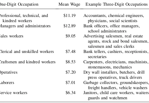
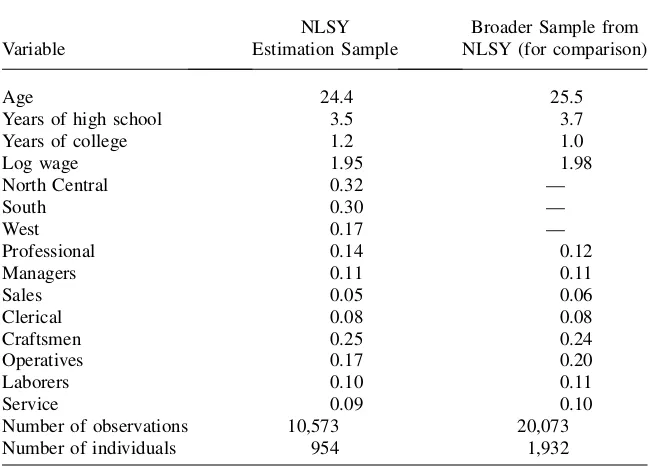
Descriptions of the one-digit occupation classifications along with average wages are presented in Table 1. The highest paid workers are professional and managerial workers, while the lowest paid workers are found in the service occupation. Descrip-tive statistics are presented in Table 2. There are 954 individuals in the estimation sample who contribute a total of 10,573 person-year observations to the data. On av-erage, each individual contributes approximately 11 observations to the data. Appen-dix 1 contains further details about the data used to estimate the model, including the details of how the sample is selected, and a discussion of the representativeness of the final sample.
A. Measurement Error in Occupation Codes
The NLSY provides the U.S. Census occupation codes for each job. Interviewers question respondents about the occupation of each job held during the year with
Table 1
Description of Occupations
One-Digit Occupation Mean Wage Example Three-Digit Occupations
Professional, technical, and kindred workers
$11.19 Accountants, chemical engineers, physicians, social scientists Managers and administrators $12.89 Bank officers, office managers,
school administrators
Sales workers $9.05 Advertising salesmen, real estate
agents, stock and bond salesmen, salesmen and sales clerks Clerical and unskilled workers $7.48 Bank tellers, cashiers, receptionists,
secretaries
Craftsmen and kindred workers $8.53 Carpenters, electricians, machinists, stonemasons, mechanics
Operatives $7.20 Dry wall installers, butchers, drill
press operatives, truck drivers
Laborers $7.01 Garbage collectors, groundskeepers,
freight handlers, vehicle washers Service workers $6.34 Janitors, child care workers, waiters,
guards and watchmen
the following two questions: What kind of work do you do? That is, what is your occupation? Coders use these descriptions to classify each job using the three-digit Census occupation coding scheme. Misclassification of occupation codes may arise from errors made by respondents when describing their job, or from errors made by coders when interpreting these descriptions. Evidence on the extent of misclassifica-tion is provided by Mellow and Sider (1983), who perform a validamisclassifica-tion study of oc-cupation codes using ococ-cupation codes found in the CPS matched with employer reports of their employee’s occupation. They find agreement rates for occupation codes of 58 percent at the narrowly defined three-digit level and 81 percent at the more broadly defined one-digit level. Additional evidence on measurement error in occupation codes is presented by Mathiowetz (1992), who independently creates one and three-digit occupation codes based on occupational descriptions from employees of a large manufacturing firm and job descriptions found in these worker’s personnel files. The agreement rate between these independently coded one-digit oc-cupation codes is 76 percent, while the agreement rate for three-digit codes is only 52 percent. In addition to comparing the three- and one-digit occupation codes produced by independent coding, Mathiowetz (1992) also conducts a direct comparison of the company record with the employee’s occupational description to see if the two sour-ces could be classified as same three-digit occupation. This direct comparison results in an agreement rate of 87 percent at the three-digit level.
Table 2
Descriptive Statistics
Variable
NLSY Estimation Sample
Broader Sample from NLSY (for comparison)
Age 24.4 25.5
Years of high school 3.5 3.7
Years of college 1.2 1.0
Log wage 1.95 1.98
North Central 0.32 —
South 0.30 —
West 0.17 —
Professional 0.14 0.12
Managers 0.11 0.11
Sales 0.05 0.06
Clerical 0.08 0.08
Craftsmen 0.25 0.24
Operatives 0.17 0.20
Laborers 0.10 0.11
Service 0.09 0.10
Number of observations 10,573 20,073
Number of individuals 954 1,932
In general, papers examining occupational choices and the returns to occupation-specific work experience have not dealt with the difficult issues raised by measurement error in occupation codes even though it is widely believed that occupation codes are quite noisy. Work by Kambourov and Manovskii (2007) is a notable exception to this trend. They exploit the fact that the Panel Study of Income Dynamics (PSID) originally coded occupations using an approach similar to the NLSY in which occupation coders translated worker’s verbatim descriptions of their occupation into an occupation code separately in each survey year. The PSID later released retrospective occupation data files where occupation coders were instead given access to a worker’s complete se-quence of occupational descriptions over his career. Kambourov and Manovskii (2007) show that occupational mobility is lower in the retrospective files, which is con-sistent with the hypothesis that coders introduce measurement error into occupation codes when they interpret workers’ verbatim job descriptions. However, it is important to note that while this type of retrospective coding is likely to reduce the number of false occupational transitions found in the data, it does not provide any additional in-formation about a worker’s true occupation. Given this limitation of the PSID data, Kambourov and Manovskii (2007) estimate the returns to occupation-specific work ex-perience, but they are not able to allow the wage equation to vary across occupations, or to estimate the importance of cross-occupation experience effects.
III. Occupational Choice Model with
Misclassification
A. A Baseline Model of Misclassification
The model of occupational choices developed in this paper builds on previous models of sectoral and occupational choices such as Heckman and Sedlacek (1985, 1990) and Gould (2002). These models are all based on the framework of self-selection in occupational choices introduced by Roy (1951). LetV
iqtrepresent the utility that workerireceives from working in occupation qat time periodt. LetN represent the number of people in the sample, let TðiÞ represent the number of time periods that personi is in the sample, and letQrepresent the number of occupations. Assume that the value of working in each occupation is the following function of the wage and nonpecuniary utility,
Viqt ¼wiqt+Hiqt+eiqt; ð1Þ
wherewiqtis the log wage of personiin occupationqat timet,Hiqtis the determin-istic portion of the nonpecuniary utility that personireceives from working in occu-pationqat timet, andeiqtis an error term that captures variation in the utility flow from working in occupationqcaused by factors that are observed by the worker but unobserved by the econometrician.
The log wage equation is
wiqt¼miq+Zitbq+ + Q
k¼1
dqkExpikt+eiqt; ð2Þ
occupationk. This specification allows for a full set of cross-occupation experience effects, so the parameter estimates provide evidence on the transferability of skills across occupations. The final term,eiqt;represents a random wage shock. The deter-ministic portion of the nonpecuniary utility flow equation for personiis specified as
Hiqt¼Xitpq+ + Q
k¼1
gqkExpikt+ + Q
k¼1
xqkLastoccikt+fiq; ð3Þ
whereXit is a vector of explanatory variables andLastoccikt is a dummy variable equal to one if personiworked in occupationkat time t21. This variable allows switching occupations to have a direct impact on nonpecuniary utility, as it would if workers incur nonpecuniary costs when switching occupations. The final term,
fiq;represents personi’s innate preference for working in occupationq. In general, sectoral choice models of this type are identified even if the same explanatory var-iables appear in both the wage equation and the nonpecuniary utility flow equation. However, it is normally considered desirable to include a variable that impacts pational choices but does not directly impact wages. In this application lagged occu-pational choice dummies and high school and college diploma dummies are included in the nonpecuniary equation but excluded from the wage equation. The exclusion of the lagged occupational choice dummies from the wage equation assumes that inviduals incur psychic mobility costs when switching occupations, but there is no di-rect monetary switching cost. However, because occupation-specific experience effects vary across occupations, when an individual switches occupations his accu-mulated skills may be valued less highly in his new occupation.4
LetOitrepresent the occupational choice observed in the data for personiat time t. This variable is an integer that takes a value ranging from one toQ. A person’s true occupational choice may differ from the one observed in the data if classification er-ror exists. LetOˆitrepresent the true occupational choice, which is simply the occu-pation that yields the highest utility,
ˆ
Oit¼q if Viqt ¼maxfVi1t ;Vi2t;.;V iQtg ð4Þ
The model of misclassification allows the probability of misclassification to depend on the value of the latent variableV
iqt. The misclassification probabilities are denoted as
ajk ¼PrðOit¼jjOˆit¼kÞ; for j¼1;.;Q k¼1;.;Q ð5Þ
That is,ajk represents the probability that the occupation observed in the data isj, conditional on the actual occupational choice beingk. Thea’s are estimated jointly along with the other parameters in the model. Theajjterms are the probabilities that occupational choices are correctly classified. There are Q3Q misclassification probabilities, but there are only½ðQ3QÞ2Qfree parameters because the misclas-sification probabilities must sum to one for each possible occupational choice,
+Qj¼1ajk¼1; for k¼1;.;Q: ð6Þ
Following existing parametric models of misclassification, the model assumes that the misclassification probabilitiesfajk : k¼1; ::;Q;j¼1;.;Qgdepend only onj andk, and not on the other explanatory variables in the model. One possible short-coming of this baseline model of occupational misclassification is that it rules out person specific heterogeneity in the propensity to misclassify occupations that may be present in panel data such as the NLSY. Section D of this paper presents an ex-tension of the model that allows for this type of within-person correlation in misclas-sification rates.
It is necessary to specify the distributions of the error terms in the model be-fore deriving the likelihood function. Assume that eiqt ; iid extreme value and eiqt;Nð0;s2eqÞ. Letfirepresent aQ31 vector of personi’s preferences for work-ing in each occupation, and letmirepresent theQ31 vector of personi’s log wage intercepts in each occupation. LetFðm;fÞdenote the joint distribution of the wage intercepts and occupational preferences.
Let u represent the vector of parameters in the model, u¼ fbk;gkj;xkj;akj;pk;djk;sek;Fðm;fÞ:k¼1;.;Q;j¼1;.;Qg. For brevity of no-tation, when it is convenient I suppress some or all of the arguments fu;Zit;Xit;Expikt;Lastoccikt;wobsit gat some points when writing equations for prob-abilities and likelihood contributions, even though the choice probprob-abilities and likeli-hood contributions are functions of all of these variables. Define Pˆitðq;wobs
it ) as the joint probability that person i chooses to work in occupation q in time period t
and receives a wage ofwobs
it . The outcome probability is ˆ
Pitðq;wobs
it jm;fÞ ¼PrðViqt ¼maxfVi1t;Vi2t;.;V
iQtgjwiqt¼wobsit Þ
3Prðwiqt¼wobsit Þ: ð7Þ
There is no closed form solution for this probability, so it is approximated using sim-ulation methods. This involves taking random draws from the distribution of the errors, and computing the mean of the simulated probabilities.5The likelihood func-tion for the observed data is constructed using the misclassificafunc-tion probabilities and the true choice probabilities. DefinePitðq;wobs
it Þas the probability that personiis ob-servedworking in occupationqat time periodtwith a wage ofwobs
it . This probability is the sum of the true occupational choice probabilities weighted by the misclassifi-cation probabilities,
Pitðq;wobsit jm;fÞ ¼ +
Q
k¼1
aqkPˆitðk;wobsit jm;fÞ: ð8Þ
Note that the outcome probability imposes the restriction that the observed wage is drawn from the worker’s actual occupation, which rules out situations where a
worker intentionally misrepresents his occupation and simultaneously provides a false wage consistent with the false occupation. The likelihood function is simply the product of the probabilities of observing the sequence of occupational choices observed in the data for each person over the years that they are in the sample,
LðuÞ ¼Y
where 1f•gdenotes the indicator function which is equal to one if its argument is true and zero otherwise. The likelihood function must be integrated over the joint distri-bution of skills and preferences,Fðm;fÞ. Following Heckman and Singer (1984), this distribution is specified as a discrete multinomial distribution.6 Suppose that there areMtypes of people, each with aQ31 vector of wage intercepts mm and
Q31 vector of preferences fm. Let vm represent the proportion of themth type in the population. The unconditional likelihood function is simply a weighted aver-age of the type specific likelihoods,
LðuÞ ¼Y
B. Evaluating the Likelihood Function
The major complication in evaluating the likelihood function arises from the fact that classification error in occupation codes creates nonclassical measurement error in the observed occupation-specific work experience variables and previous occupational choice dummy variables that describe an individual’s state. This implies that the true state of each agent is unobserved. Previous research into occupational choices has not addressed this issue. The key to understanding the solution to this problem is to realize that the model of misclassification implies a distribution of true values of occupation-specific work experience and lagged occupational choices for each in-dividual in each time period. Estimating the parameters of the model by maximum likelihood involves integrating over the distribution of these unobserved state varia-bles. However, there is no closed form solution for this integral, and, more impor-tantly, the distribution is intractably complex. These problems are solved by
simulating the likelihood function. The algorithm involves recursively simulatingR
sequences of occupation-specific work experience and lagged occupational choices that span a worker’s entire career. The individual’s likelihood contribution is com-puted for each simulated sequence, and the path probabilities are averaged over theRsequences to obtain the simulated likelihood contribution. A detailed descrip-tion of the simuladescrip-tion algorithm is presented in Appendix 2.
C. Identification
This section presents the identification conditions for the occupational choice model with misclassification and discusses several related issues.
1. Identification Conditions
The identification conditions for a model of misclassification in a binary dependant variable are presented by Hausman, Abrevaya, and Scott-Morton (1998). This con-dition is extended to the case of discrete choice models with more than two outcomes by Ramalho (2002). The parameters of the model are identified if the sum of the con-ditional misclassification probabilities for each observed outcome is smaller than the conditional probability of correct classification. In the context of the occupational choice model presented in this paper this condition amounts to the following restric-tion on the misclassificarestric-tion probabilities,
+
k6¼j
ajk,ajj; j¼1;.;Q: ð12Þ
This condition implies that it is not possible to estimate the extent of misclassifica-tion along with the rest of the parameter vector if the quality of the data is so poor that one is more likely to observe a misclassified occupational choice than a correctly classified occupational choice.
2. Discussion
Estimating the extent of classification error in the NLSY occupation data along with the parameters of the occupational choice model is only possible if one is willing to adopt a parametric model along with the associated functional form and distribu-tional assumptions.7It is worthwhile to consider at an intuitive level how the para-metric occupational choice model and misclassification model are linked together. Let ˜brepresent the parameter vector for the occupational choice model, and let ˜a
represent the vector of misclassification parameters. Given ˜bthe parametric model of occupational choices provides the probability that each occupational choice and wage combination observed in the NLSY is generated by the model. Taking ˜b as given, one could choose the value of ˜athat maximizes the probability of observing the NLSY occupation and wage data. Broadly speaking, this will happen when the combinations of occupational choices and wages that are unlikely to be generated by the model at the parameter vector ˜bare assigned a relatively high probability of being affected by misclassification. During estimation, ˜b is not fixed, it is
estimated simultaneously with ˜a, so estimating the model amounts to choosing the value of ˜bthat best fits the data, with the added consideration that the chosen value of ˜aallows misclassification to account for some of the observed patterns in the data. Existing parametric models of misclassification estimate misclassification rates using discrete choice models, while in contrast this paper jointly models discrete oc-cupational choices along with wages. The advantage of this approach is that to the extent that wages vary across occupations, observed wages provide information about which observed choices are likely to be affected by misclassification.8This ap-proach uses information about the relationship between observable variables (such as education) and occupational choices, along with information about the consistency of observed wages with reported occupations to infer the extent of misclassification in the data. It should be noted that when occupations are measured with error, it is not possible to nonparametrically determine the exact relationship between true oc-cupational choices, wages, and observable variables such as education. However, within a particular parametric model of occupational choices and wages, these parameters can be estimated.9
The availability of validation data on occupations from an outside data source would, in principle, allow one to relax some of the parametric assumptions adopted in this paper. For example, if another data set contained information about reported occupations, true occupations, and possibly other explanatory variables, this informa-tion could be used to integrate out the effect of measurement error. Of course, this ap-proach relies on the assumption that the measurement error process is identical in the two sources of data. While this approach appears promising and is certainly worth pur-suing in future research, on a practical level adopting this approach would most likely require additional data collection that was targeted specifically at validating occupation codes.10 One possible approach would be to validate an individual’s occupation by
8. In the extreme case where the wage distribution is identical across occupations observed wages do not provide any additional information about misclassification. However, even if the unconditional wage dis-tribution is identical across occupations, if the wage disdis-tribution in each occupation is a function of observ-able characteristics (such as education and occupation-specific experience), and the effects of these variables on wages vary across occupations, then observed wages will still provide information about mis-classification.
9. Although panel data is used to estimate the model, it is also possible to estimate this type of model using cross-sectional data. As an experiment, I randomly selected a cross-section of workers from the panel data NLSY sample and reestimated the model. The estimated level of misclassification in the cross-sectional version of the model was 8 percent, compared to 9 percent in the panel data version. The fact that these estimates are so close suggests that misclassification rates are primarily identified by the consistency of an individual’s reported occupation with the cross-sectional distribution of choices, wages, and observable variables, rather than by the extent to which an observed occupational choice is consistent with an individ-ual worker’s observed sequence of career choices.
questioning his supervisor, since presumably supervisors know the type of work per-formed by workers that they manage. This approach would circumvent some of the problems associated with validating occupation codes using personnel records, which may or may not contain job descriptions that accurately reflect occupations.
D. An Extended Model: Heterogeneity in Misclassification Rates
The model of misclassification presented in Section III, Subsection A assumes that all individuals have the same probability of having one of their occupational choices misclassified. In a panel data setting such as the NLSY, it is possible that during the yearly NLSY interviews some individuals consistently provide poor descriptions of their jobs that are likely to lead to measurement error in the occupation codes created by the NLSY coders. On the other hand, some workers may be more likely to provide accurate descriptions of their occupations that are extremely unlikely to be misclas-sified. The remainder of this section extends the occupational choice model with mis-classification to allow for time persistent mismis-classification by using an approach similar to the one adopted by Dustmann and van Soest (2001) in their study of mis-classification of language fluency.
The primary goal of the extended model is to allow for person-specific heteroge-neity in misclassification rates in a way that results in a tractable empirical model. Suppose that there are three subpopulations of workers in the economy, and that these subpopulations each have different probabilities of having their occupational choices misclassified. Define the occupational choice misclassification probabilities for Subpopulationyas
ajkðyÞ ¼PrðOit¼jjOˆit¼kÞ; j¼1;.;Q k¼1;.;Q ð13Þ
+
Q
j¼1
ajkðyÞ ¼1 k¼1;.;Q; y¼1;2;3: ð14Þ
Denote the proportion of Subpopulationyin the economy asjðyÞ,wherey¼1;2;3 and+3y¼1jðyÞ ¼1. This specification of the misclassification rates allows for time-persistence in misclassification, since theajkðyÞ’s are fixed over time for each sub-population. During estimation the jðyÞ’s and ajkðyÞ’s of each subpopulation are estimated along with the other parameters of the model, so it is necessary to specify the misclassification model in such a way that the number of parameters in the model does not become unreasonably large. In order to keep the number of parameters at a tractable level, the number of subpopulations is set to a small number (3), and the misclassification probabilities are restricted during estimation so that the occupa-tional choices of subpopulation one are always correctly classified.11
This model of misclassification incorporates the key features of heterogeneous misclassification rates in a fairly parsimonious way. Some fraction of the population (jð1Þ) is always correctly classified, and the remaining two subpopulations are allowed to have completely different misclassification rates, so that both the overall
level of misclassification and the particular patterns in misclassification are allowed to vary between subpopulations.
The likelihood function presented in Section III, Subsection A can be modified to account for person-specific heterogeneity in misclassification. The observed choice probabilities are easily modified so that they are allowed to vary by subpopulation,
Pitðq;wobsit jm;f;yÞ ¼ +Q
k¼1
aqkðyÞPˆitðk;wobsit jm;fÞ; ð15Þ
wherey¼1,.,3indexes subpopulations. Conditional on subpopulations, the likeli-hood function is
The subpopulation that a particular person belongs to is not observed, so the likeli-hood function must be integrated over the discrete distribution of the type-specific misclassification rates,
This section presents the simulated maximum likelihood parameter estimates for the occupational choice model. First, the parameters that reveal the ex-tent of classification error in reported occupations are discussed, and then the param-eter estimates from the occupational choice model that corrects for classification error and allows for person-specific heterogeneity in misclassification are compared to the estimates from a model that does not correct for measurement error. Next, the sensitivity of the estimates to measurement error in wages is examined. Finally, the model is used to simulate data that is free from classification error in occupation codes.
A. The Extent of Measurement Error in Occupation Codes
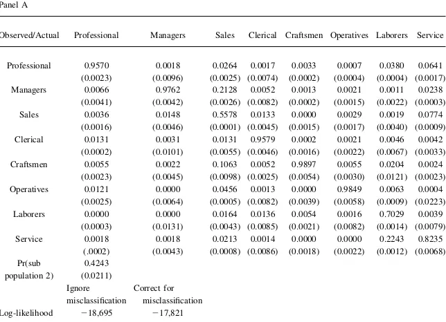
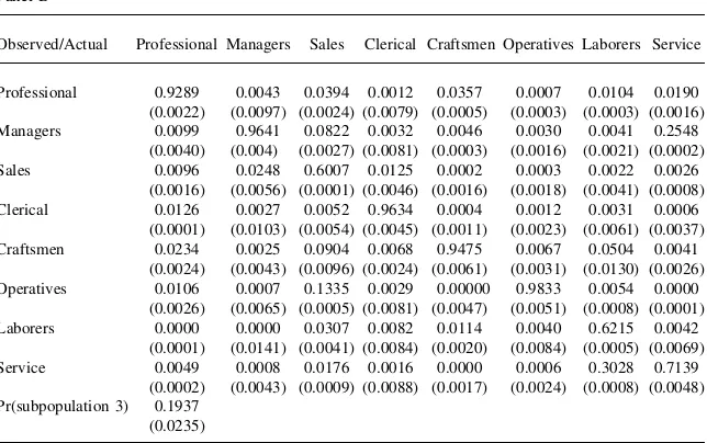
the estimate ofaijðyÞ, which is the probability that occupationiis observed in the data conditional on occupationjbeing the actual choice for a person in Subpopula-tiony. For example, the entry in the third column of the first row indicates that con-dition of being a member of Subpopulation 2, there is a 2.6 percent chance that a person who is actually a sales worker will be misclassified as a professional worker. The diagonal elements of the two panels of Table 4 show the probabilities that oc-cupational choices are correctly classified. Averaged across all occupations, the prob-ability that an occupational choice is correctly classified is 0.868 for Subpopulation 2 and 0.840 for Subpopulation 3. One striking feature of the estimated misclassifica-tion probabilities is that they provide substantial evidence that misclassificamisclassifica-tion rates vary widely across occupations. For example, in Subpopulation 2 the probability that an occupational choice is correctly classified ranges from a low of 0.56 for sales workers to a high of 0.99 for craftsmen, while in Subpopulation 3 the probability that an occupational choice is correctly classified ranges from a low of 0.60 for sales workers to a high of 0.98 for operatives.
The estimates of the probabilities that a person belongs to Subpopulations 2 and 3 are 42 percent and 19 percent, which leaves an estimated 38 percent of the popula-tion belonging to Subpopulapopula-tion 1, the group whose occupapopula-tional choices are never misclassified. The fact that a substantial fraction of the population belongs to the sub-population whose occupational choices are never misclassified highlights the impor-tance of allowing for person-specific heterogeneity in misclassification rates. When averaged over subpopulations, the subpopulation-specific misclassification rates Table 3
Occupational Transition Matrix—NLSY Data (top entry) and Simulated Data (bottom entry)
Professional Managers Sales Clerical Craftsmen Operatives Laborers Service
Professional 74.7 6.9 2.3 4.5 5.0 3.0 1.3 2.2
78.5 5.6 4.2 3.7 3.2 2.2 1.4 1.2
Managers 6.4 57.4 7.2 7.3 10.7 3.5 2.5 5.0
6.6 58.5 9.4 7.4 10.3 2.9 2.6 2.3
Sales 8.0 14.9 53.5 7.7 5.4 5.2 2.2 3.2
7.6 9.2 55.2 6.3 6.8 5.9 5.2 3.6
Clerical 10.3 12.4 5.9 44.8 6.8 7.0 8.3 4.6
8.7 11.4 7.2 45.8 6.3 6.8 9.8 4.0
Craftsmen 2.9 5.3 1.0 2.2 66.6 11.1 8.1 2.6
2.0 4.7 2.3 2.0 67.4 10.8 9.6 1.2
Operatives 2.4 2.2 2.1 3.1 18.4 56.8 10.1 4.9
1.9 1.3 3.3 2.9 18.3 56.3 11.6 4.4
Laborers 2.7 3.3 1.8 7.9 23.2 18.6 36.2 6.1
2.5 2.7 4.0 7.3 21.6 16.5 39.1 6.2
Service 3.9 7.8 1.5 3.5 8.4 6.8 8.6 59.5
3.7 4.2 2.8 3.1 6.8 6.2 9.5 63.7
Total 14.0 11.5 5.3 7.6 25.8 16.9 9.6 9.4
13.9 9.5 7.9 7.3 25.2 16.2 11.5 8.4
indicate that 91 percent of one-digit occupational choices are correctly classified. This estimate of the overall extent of misclassification in the NLSY data is lower than the misclassification rates reported in validation studies based on other datasets. For example, Mellow and Sider (1983) find an agreement rate of 81 percent at the one-digit level between employee’s reported occupations and employer’s oc-cupational descriptions in the January 1977 Current Population Survey (CPS). Mathiowetz (1992) finds a 76 percent agreement rate between the occupational descriptions given by workers of a single large manufacturing firm and personnel records.12
One possible explanation for the lower misclassification rate found in this study compared to the validation studies is that the NLSY occupation data is of higher qual-ity than both the CPS data and the survey conducted by Mathiowetz (1992). It appears that the procedures used by the CPS and NLSY in constructing occupation codes are quite similar, so it is not clear that one should expect the NLSY data to Table 4
Parameter Estimates- Misclassification Probabilities for Subpopulation 2 (ajk(2))
Panel A
Observed/Actual Professional Managers Sales Clerical Craftsmen Operatives Laborers Service Professional 0.9570 0.0018 0.0264 0.0017 0.0033 0.0007 0.0380 0.0641 (0.0023) (0.0096) (0.0025) (0.0074) (0.0002) (0.0004) (0.0004) (0.0017) Managers 0.0066 0.9762 0.2128 0.0052 0.0013 0.0021 0.0011 0.0238
(0.0041) (0.0042) (0.0026) (0.0082) (0.0002) (0.0015) (0.0022) (0.0003) Sales 0.0036 0.0148 0.5578 0.0133 0.0000 0.0029 0.0019 0.0774
(0.0016) (0.0046) (0.0001) (0.0045) (0.0015) (0.0017) (0.0040) (0.0009) Clerical 0.0131 0.0031 0.0131 0.9579 0.0002 0.0021 0.0046 0.0042
(0.0002) (0.0101) (0.0055) (0.0046) (0.0016) (0.0022) (0.0067) (0.0033) Craftsmen 0.0055 0.0022 0.1063 0.0052 0.9897 0.0055 0.0204 0.0024
(0.0023) (0.0045) (0.0098) (0.0025) (0.0054) (0.0030) (0.0121) (0.0023) Operatives 0.0121 0.0000 0.0456 0.0013 0.0000 0.9849 0.0063 0.0004
(0.0025) (0.0064) (0.0005) (0.0082) (0.0039) (0.0058) (0.0009) (0.0223) Laborers 0.0000 0.0000 0.0164 0.0136 0.0054 0.0016 0.7029 0.0039
(0.0003) (0.0131) (0.0043) (0.0085) (0.0021) (0.0082) (0.0014) (0.0079) Service 0.0018 0.0018 0.0213 0.0014 0.0000 0.0000 0.2243 0.8235
(.0002) (0.0043) (0.0008) (0.0086) (0.0018) (0.0022) (0.0012) (0.0068) Pr(sub
population 2)
0.4243 (0.0211) Ignore misclassification
Correct for misclassification Log-likelihood 218,695 217,821
Notes: Elementa(i,j)of this table, whereirefers to the row andjrefers to the column is the probability that occupationiis observed, conditional onjbeing the true choice:a(j,k)¼Pr(occupation j observed | occu-pation k is true choice).Standard errors in parentheses. ‘‘Subpopulation’’ refers to the fact that the misclas-sification model allows for heterogeneity in misclasmisclas-sification rates.
have a lower misclassification rate than the CPS. An alternative explanation is that the employer reports of occupation codes that are assumed to be completely free from classification error in validation studies are in fact measured with error.13If this is true, then comparing noisy self-reported data to noisy employer reported data would cause validation studies to overstate the extent of classification error in occu-pation codes. The idea that this type of validation study may result in an overstate-ment of classification error in occupation or industry codes is not a new one. For example, Krueger and Summers (1988) assume that the error rate for one-digit indus-try classifications is half as large as the one reported by Mellow and Sider (1983) as a rough correction for the overstatement of classification error in validation studies.
The wide variation in misclassification rates across occupations along with the pat-terns in misclassification suggest that certain types of jobs are likely to be misclas-sified in particular directions. In addition, the misclassification matrix is highly asymmetric. For example, there is only a 1.4 percent chance that a manager will be misclassified as a sales worker, but there is a 21 percent chance that a sales worker Table 4
Misclassification Probabilities for Subpopulation 3 (aij(3))
Panel B
Observed/Actual Professional Managers Sales Clerical Craftsmen Operatives Laborers Service
Professional 0.9289 0.0043 0.0394 0.0012 0.0357 0.0007 0.0104 0.0190 (0.0022) (0.0097) (0.0024) (0.0079) (0.0005) (0.0003) (0.0003) (0.0016)
Managers 0.0099 0.9641 0.0822 0.0032 0.0046 0.0030 0.0041 0.2548
(0.0040) (0.004) (0.0027) (0.0081) (0.0003) (0.0016) (0.0021) (0.0002)
Sales 0.0096 0.0248 0.6007 0.0125 0.0002 0.0003 0.0022 0.0026
(0.0016) (0.0056) (0.0001) (0.0046) (0.0016) (0.0018) (0.0041) (0.0008)
Clerical 0.0126 0.0027 0.0052 0.9634 0.0004 0.0012 0.0031 0.0006
(0.0001) (0.0103) (0.0054) (0.0045) (0.0011) (0.0023) (0.0061) (0.0037)
Craftsmen 0.0234 0.0025 0.0904 0.0068 0.9475 0.0067 0.0504 0.0041
(0.0024) (0.0043) (0.0096) (0.0024) (0.0061) (0.0031) (0.0130) (0.0026) Operatives 0.0106 0.0007 0.1335 0.0029 0.00000 0.9833 0.0054 0.0000
(0.0026) (0.0065) (0.0005) (0.0081) (0.0047) (0.0051) (0.0008) (0.0001)
Laborers 0.0000 0.0000 0.0307 0.0082 0.0114 0.0040 0.6215 0.0042
(0.0001) (0.0141) (0.0041) (0.0084) (0.0020) (0.0084) (0.0005) (0.0069)
Service 0.0049 0.0008 0.0176 0.0016 0.0000 0.0006 0.3028 0.7139
(0.0002) (0.0043) (0.0009) (0.0088) (0.0017) (0.0024) (0.0008) (0.0048) Pr(subpopulation 3) 0.1937
(0.0235)
Notes: Elementa(i,j)of this table, whereirefers to the row andjrefers to the column is the probability that occupationiis observed, conditional onjbeing the true choice:a(j,k)¼Pr(occupation j observed | occu-pation k is true choice).Standard errors in parentheses. ‘‘Subpopulation’’ refers to the fact that the misclas-sification model controls for unobserved heterogeneity in misclasmisclas-sification rates by allowing for a discrete number of subpopulations that are each allowed to have different misclassification matrices.
will be misclassified as a manager. Reading down the laborers column of Panel A of Table 4 shows that laborers are frequently misclassified as service workers (22 cent), but service workers are very unlikely to be misclassified as laborers (.39 per-cent). Further evidence of asymmetric misclassification is found throughout Table 4.
B. Occupational Choice Model Parameter Estimates
The parameter estimates for the occupational choice model estimated with and with-out correcting for classification error are presented in Table 5. In addition, this table presents a measure of the difference between each parameter in the baseline (bb) and
Table 5
Age 0.0233 0.0079 0.0474 0.0351
(0.0154) (0.0073) 2.12 (0.0184) (0.0091) 1.35
Age2/100 20.2280 20.1434 20.4028 20.3543
(0.0985) (0.0426) 21.98 (0.1230) (0.0630) 20.77
Education 0.0734 0.0626 0.0825 0.0837
(0.0057) (0.0041) 2.66 (0.0082) (0.0060) 20.20
Professional experience 0.0715 0.0687 0.0944 0.0896
(0.0053) (0.0034) 0.81 (0.0130) (0.0086) 0.56
Managerial experience 0.0375 0.0644 0.0656 0.0547
(0.0158) (0.0123) 22.19 (0.0071) (0.0055) 1.99
Sales experience 0.0493 0.0499 0.0888 0.0879
(0.0147) (0.0101) 20.06 (0.0135) (0.0097) 0.09
Clerical experience 0.0430 0.0377 0.0191 0.0209
(0.0191) (0.0162) 0.33 (0.0096) (0.0073) 20.25
Craftsmen experience 0.0280 0.0203 0.0488 0.0556
(0.0092) (0.0100) 0.77 (0.0074) (0.0062) 21.10
Operatives experience 0.0447 0.0259 0.0634 0.0705
(0.0236) (0.0210) 0.90 (0.0124) (0.0121) 20.59
Laborer experience 0.0146 20.0083 0.0416 0.0233
(0.0291) (0.0232) 0.99 (0.0268) (0.0179) 1.02
Service experience 0.0000 0.0718 0.0100 0.0069
(0.0224) (0.0234) 23.07 (0.0140) (0.0117) 0.26
North central 20.0635 20.0139 20.1063 20.0667
(0.0262) (0.0189) 22.63 (0.0302) (0.0233) 21.70
South 20.0448 0.0222 20.0726 20.0849
(0.0245) (0.0182) 23.69 (0.0345) (0.0284) 0.43
West 0.0412 0.1046 20.0919 20.0531
(0.0294) (0.0205) 23.09 (0.0438) (0.0311) 21.25
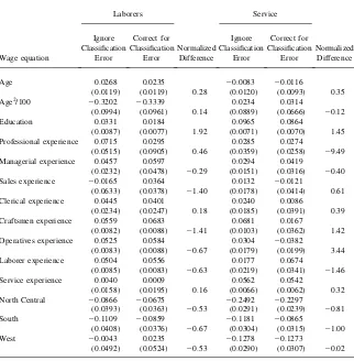
classification error (bce) models,ðbb2bceÞ=seðbceÞ, where seðbceÞ is the standard error ofbce. In the remainder of the paper this standard error normalized difference will be referred to as the normalized change in the parameter.
1. Wage Equation
While theoretical results regarding the effects of measurement error in simple linear models have been derived, there are no clear predictions for nonlinear models such as this occupational choice model. Broadly speaking, one would expect the patterns of Table 5
Age 0.0662 0.1354 0.0480 0.0413
(0.0368) (0.0272) 22.55 (0.0153) (0.0157) 0.43
Age2/100 21.0006 21.0984 20.4330 20.3588
(0.2662) (0.1886) 0.52 (0.1057) (0.1095) 20.68
Education 0.1837 0.1593 0.0528 0.0511
(0.0189) (0.0268) 0.91 (0.0087) (0.0081) 0.21
Professional experience 0.0672 0.0308 0.0957 0.1051
(0.0366) (0.0542) 0.67 (0.0146) (0.0230) 20.41
Managerial experience 0.1316 0.1089 0.0454 0.0418
(0.0274) (0.0322) 0.71 (0.0104) (0.0121) 0.30
Sales experience 0.1774 0.1571 0.0806 0.0888
(0.0163) (0.0195) 1.04 (0.0162) (0.0203) 20.40
Clerical Experience 0.1281 0.0430 0.0562 0.0572
(0.0333) (0.0433) 1.97 (0.0085) (0.0093) 20.11
Craftsmen experience 20.0183 20.0453 0.0502 0.0646
(0.0258) (0.0297) 0.91 (0.0083) (0.0119) 21.21
Operatives experience 0.0845 0.0845 0.0516 0.0500
(0.0284) (0.0297) 0.00 (0.0118) (0.0125) 0.13
Laborer experience 0.0507 0.0521 0.0420 0.0345
(0.0431) (0.0552) 20.03 (0.0167) (0.0153) 0.49
Service experience 0.0241 20.0657 0.0191 0.0215
(0.0295) (0.0826) 1.09 (0.0177) (0.0183) 20.13
North Central 20.2505 20.3711 20.1688 20.1965
(0.0754) (0.1051) 1.15 (0.0311) (0.0369) 0.75
South 0.1225 0.1249 20.0847 20.1030
(0.0764) (0.0915) 20.03 (0.0307) (0.0377) 0.49
West 0.0979 0.1015 20.0228 20.0230
(0.0945) (0.1070) 20.03 (0.0342) (0.0362) 0.01
misclassification present in the data to be a key determinant of the magnitude and direction of the resulting bias. Due to the large number of wage equation parameters, this discussion focuses on a small subset of parameter estimates with the goal of demonstrating that classification error is something that needs to be accounted for when estimating occupation-specific wage equations. In addition, this discussion will attempt to highlight the type of questions in general that one might receive mislead-ing answers to if one examines occupational choices and ignores misclassification.
The wage equation parameter estimates are presented in Panel A of Table 5. The estimates of the wage equation for the professional occupation show a number of Table 5
Age 0.0606 0.0489 0.0128 0.0123
(0.0068) (0.0053) 2.21 (0.0085) (0.0073) 0.07
Age2/100 20.5257 20.4576 20.2230 20.2605
(0.0481) (0.0398) 21.71 (0.0642) (0.0604) 0.62
Education 0.0290 0.0254 0.0209 0.0079
(0.0048) (0.0045) 0.80 (0.0054) (0.0048) 2.74
Professional experience 0.0290 0.0188 0.0670 0.0751
(0.0120) (0.0210) 0.49 (0.0229) (0.0344) 20.24
Managerial experience 0.0558 0.0646 0.0432 0.0552
(0.0115) (0.0113) 20.78 (0.0157) (0.0152) 20.79
Sales experience 0.0100 0.0438 0.0200 0.0157
(0.0169) (0.0183) 21.85 (0.0149) (0.0176) 0.24
Clerical experience 0.0381 0.0366 0.0499 0.0370
(0.0125) (0.0210) 0.07 (0.0110) (0.0191) 0.68
Craftsmen experience 0.0591 0.0605 0.0607 0.0764
(0.0028) (0.0027) 20.52 (0.0067) (0.0062) 22.52
Operatives experience 0.0386 0.0352 0.0549 0.0470
(0.0052) (0.0048) 0.71 (0.0045) (0.0041) 1.92
Laborer experience 0.0217 0.0114 0.0708 0.0512
(0.0069) (0.0066) 1.57 (0.0090) (0.0077) 2.56
Service experience 0.0254 0.0361 20.0023 0.0285
(0.0094) (0.0106) 21.00 (0.0149) (0.0147) 22.10
North Central 20.1034 20.1201 20.0637 20.0948
(0.0197) (0.0185) 0.91 (0.0266) (0.0222) 1.40
South 20.0786 20.0828 0.0234 0.0026
(0.0209) (0.0182) 0.23 (0.0270) (0.0222) 0.94
West 0.0847 0.0868 0.0086 20.0043
(0.0210) (0.0208) 20.10 (0.0307) (0.0268) 0.48
large changes in the estimated effects of occupation-specific work experience on wages between the model that ignores classification error in occupations and the one that accounts for classification error. For example, the effect of a year of man-agerial experience on wages in the professional occupation is biased downward by 42 percent from 0.064 to 0.037 when misclassification is ignored. The standard error normalized difference for this parameter is -2.19, so the bias appears relatively large relative to the standard error. The bias in this particular parameter is also interesting because the estimated misclassification probabilities show that professionals are rarely misclassified as managers (a21ð2Þ ¼0:0066,a21ð3Þ ¼0:0099), and managers
Age 0.0268 0.0235 20.0083 20.0116
(0.0119) (0.0119) 0.28 (0.0120) (0.0093) 0.35
Age2/100 20.3202 20.3339 0.0234 0.0314
(0.0994) (0.0961) 0.14 (0.0889) (0.0666) 20.12
Education 0.0331 0.0184 0.0965 0.0864
(0.0087) (0.0077) 1.92 (0.0071) (0.0070) 1.45
Professional experience 0.0715 0.0295 0.0285 0.0274
(0.0515) (0.0905) 0.46 (0.0359) (0.0258) 29.49
Managerial experience 0.0457 0.0597 0.0294 0.0419
(0.0232) (0.0478) 20.29 (0.0151) (0.0316) 20.40
Sales experience 20.0165 0.0364 0.0132 20.0121
(0.0633) (0.0378) 21.40 (0.0178) (0.0414) 0.61
Clerical experience 0.0445 0.0401 0.0240 0.0086
(0.0234) (0.0247) 0.18 (0.0185) (0.0391) 0.39
Craftsmen experience 0.0559 0.0683 0.0681 0.0167
(0.0082) (0.0088) 21.41 (0.0103) (0.0362) 1.42
Operatives experience 0.0525 0.0584 0.0304 20.0382
(0.0083) (0.0088) 20.67 (0.0179) (0.0199) 3.44
Laborer experience 0.0504 0.0556 0.0177 0.0674
(0.0085) (0.0083) 20.63 (0.0219) (0.0341) 21.46
Service experience 0.0040 0.0009 0.0562 0.0542
(0.0158) (0.0195) 0.16 (0.0066) (0.0062) 0.32
North Central 20.0866 20.0675 20.2492 20.2297
(0.0393) (0.0363) 20.53 (0.0291) (0.0239) 20.81
South 20.1109 20.0859 20.1181 20.0865
(0.0408) (0.0376) 20.67 (0.0304) (0.0315) 21.00
West 20.0043 0.0235 20.1278 20.1273
(0.0492) (0.0524) 20.53 (0.0290) (0.0307) 20.02
are rarely misclassified as professionals (a12ð2Þ ¼0:0018, a12ð3Þ ¼0:0043). The low misclassification rates between these occupations combined with the large bias in the experience coefficient illustrates the point that even a small amount of misclas-sification can produce large biases in estimates of the transferability of human capital across occupations.
Sales workers are the most frequently misclassified workers in both Subpopula-tions 2 and 3. Averaged across all three subpopulaSubpopula-tions, only 72 percent of sales workers are correctly classified. In the most common subpopulation, sales workers are most likely to be misclassified as managers (a23ð2Þ ¼0:21), so one might expect significant bias in estimates of the parameters of the managerial and sales wage equa-tions. The estimates show that ignoring classification error causes the value of expe-rience as a manager in the managerial occupation to be overstated by 19 percent (normalized change¼1.99). In addition, ignoring classification error leads to the misleading conclusion that one year of clerical experience increases wages by nearly 13 percent in the sales occupation, and this effect is statistically significant at the 5 percent level. However, once classification error is corrected for, the estimated effect of clerical experience on sales wages falls by 2/3, and the effect is not statistically different at conventional levels. Similarly, ignoring classification error leads to an overstatement in the value of professional experience in the sales occupation (0.0672 vs. 0.0308), although the normalized difference for this parameter is only 0.67.
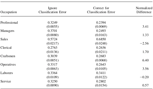
Table 5
Parameter Estimates—Error Standard Deviations
Panel A
Occupation
Ignore Classification Error
Correct for Classification Error
Normalized Difference
Professional 0.3249 0.2394
(0.0055) (0.0069) 3.41
Managers 0.3701 0.2493
(0.0080) (0.0163) 1.33
Sales 0.5724 0.6850
(0.0217) (0.0248) 22.56
Clerical 0.2763 0.2636
(0.0136) (0.0211) 1.70
Craftsmen 0.3039 0.2683
(0.0051) (0.0068) 6.40
Operatives 0.3317 0.2643
(0.0063) (0.0105) 3.56
Laborers 0.3364 0.3411
(0.0109) (0.0122) 20.20
Service 0.3250 0.2802
(0.0090) (0.0154) 0.57
Table 5
Age 0.1203 0.0973 20.0409 20.1448
(0.0799) (0.0305) 0.75 (0.0809) (0.0551) 21.40
Age2/100 20.2295 20.0345 0.4907 1.0633
(0.6142) (0.2001) 0.97 (0.5784) (0.4094) 22.02
Education 0.4260 0.4715 0.2145 0.2631
(0.0543) (0.0370) 21.23 (0.0570) (0.0240) 0.35
High school diploma 20.6393 20.3529 20.2384 20.3125
(0.2354) (0.2103) 21.36 (0.2213) (0.2106) 20.99
College diploma 0.0984 0.3509 0.2867 0.5197
(0.1881) (0.2144) 21.18 (0.2013) (0.2353) 20.46
Professional experience 0.4819 0.4894 0.3134 0.3707
(0.1484) (0.1162) 20.06 (0.1468) (0.1250) 20.63
Managerial experience 20.0761 20.0229 0.2605 0.3433
(0.0830) (0.1472) 20.36 (0.0688) (0.1308) 20.17
Sales experience 20.1569 20.1803 0.0811 0.1052
(0.1171) (0.1604) 0.15 (0.1009) (0.1430) 20.75
Clerical experience 20.1028 20.0184 0.1471 0.2410
(0.1126) (0.1637) 20.52 (0.0860) (0.1249) 21.08
Craftsmen experience 0.1531 0.2813 0.2197 0.3523
(0.0657) (0.1271) 21.01 (0.0579) (0.1224) 21.06
Operatives experience 20.1836 20.1056 0.0218 0.1383
(0.0874) (0.1784) 20.44 (0.0608) (0.1102) 21.39
Laborer experience 20.0459 0.1008 20.0207 0.2366
(0.1420) (0.2052) 20.71 (0.1182) (0.1849) 0.10
Service experience 20.4737 20.8955 20.2765 20.2843
(0.0645) (0.1467) 2.88 (0.0574) (0.0820) 21.62
Previously a professional 2.469 3.108 1.237 2.022
(0.339) (0.368) 21.74 (0.379) (0.484) 21.47
Previously a manager 0.792 1.181 2.780 3.717
(0.340) (0.665) 20.59 (0.261) (0.636) 0.14
Previously sales 1.194 0.893 1.703 1.623
(0.459) (0.594) 0.51 (0.432) (0.591) 21.20
Previously clerical 1.628 1.546 1.853 2.198
(0.354) (0.364) 0.22 (0.322) (0.287) 21.71
Previously a craftsman 1.042 1.064 1.673 2.482
(0.298) (0.485) 20.05 (0.294) (0.472) 20.18
Previously an operative 0.752 0.537 0.400 0.493
(0.305) (0.488) 0.44 (0.320) (0.516) 20.20
Previously a laborer 0.634 0.341 0.839 0.931
(0.346) (0.509) 0.58 (0.333) (0.471) 1.89
Table 5
Age 20.1327 20.3511 20.1327 20.3511
(0.1137) (0.0484) 4.52 (0.1137) (0.0484) 1.38
Age2/100 1.3350 2.8694 1.3350 2.8694
(0.8122) (0.4692) 23.27 (0.8122) (0.4692) 21.19
Education 0.1403 0.1338 0.1403 0.1338
(0.0764) (0.0563) 0.12 (0.0764) (0.0563) 0.28
High school diploma 20.0762 20.3263 20.0762 20.3263
(0.3236) (0.2981) 0.84 (0.3236) (0.2981) 0.15
College diploma 0.6676 0.9465 0.6676 0.9465
(0.2308) (0.2761) 21.01 (0.2308) (0.2761) 21.04
Professional experience 0.0865 0.0444 0.0865 0.0444
(0.1731) (0.1797) 0.23 (0.1731) (0.1797) 0.08
Managerial experience 0.0223 0.0827 0.0223 0.0827
(0.0903) (0.1555) 20.39 (0.0903) (0.1555) 20.40
Sales experience 0.1072 0.0814 0.1072 0.0814
(0.1016) (0.1502) 0.17 (0.1016) (0.1502) 0.34
Clerical experience 20.0090 0.0779 20.0090 0.0779
(0.1083) (0.1501) 20.58 (0.1083) (0.1501) 20.53
Craftsmen experience 0.1471 0.3264 0.1471 0.3264
(0.0948) (0.1370) 21.31 (0.0948) (0.1370) 20.70
Operatives experience 0.0325 0.1358 0.0325 0.1358
(0.0869) (0.1214) 20.85 (0.0869) (0.1214) 21.20
Laborer experience 20.0951 0.0596 20.0951 0.0596
(0.1618) (0.1700) 20.91 (0.1618) (0.1700) 20.87
Service experience 20.3775 20.4288 20.3775 20.4288
(0.0972) (0.1928) 0.27 (0.0972) (0.1928) 20.25
Previously a professional 1.312 1.934 1.312 0.1934
(0.476) (0.599) 21.04 (0.476) (0.0599) 21.11
Previously a manager 1.837 2.194 1.837 2.194
(0.393) (0.735) 20.49 (0.393) (0.735) 20.85
Previously sales 3.262 2.869 3.262 2.869
(0.411) (0.544) 0.72 (0.411) (0.544) 0.48
Previously clerical 2.005 1.864 2.005 1.864
(0.388) (0.0427) 0.33 (0.388) (0.427) 20.73
Previously a craftsman 1.358 1.778 1.358 1.778
(0.407) (0.573) 20.73 (0.407) (0.573) 20.72
Previously an operative 1.272 1.049 1.272 1.049
(0.361) (0.457) 0.49 (0.361) (0.457) 0.37
Previously a laborer 1.358 1.015 1.358 1.015
(0.457) (0.545) 0.63 (0.457) (0.545) 0.65
Table 5
Age 20.1896 20.2998 20.1519 20.2535
(0.0717) (0.0799) 1.82 (0.0551) (0.0558) 1.87
Age2/100 1.1693 1.8996 1.3557 2.0207
(0.5598) (0.6139) 21.43 (0.4459) (0.4634) 21.51
Education 0.1443 0.1253 20.0703 20.0873
(0.0638) (0.0678) 0.40 (0.0479) (0.0422) 0.36
High school diploma 0.2760 0.2466 0.1959 0.1931
(0.2437) (0.1995) 0.02 (0.1839) (0.1680) 20.09
College diploma 0.5009 0.7951 20.4700 20.4137
(0.2163) (0.2838) 20.16 (0.2633) (0.3614) 20.05
Professional experience 0.1874 0.1779 0.1858 0.1962
(0.1529) (0.1211) 20.08 (0.1581) (0.1387) 0.79
Managerial experience 0.0188 0.0697 20.1568 20.0980
(0.0762) (0.1283) 20.45 (0.0753) (0.1321) 0.00
Sales experience 20.1264 20.1851 20.2418 20.3401
(0.1093) (0.1752) 0.54 (0.1272) (0.1816) 20.14
Clerical experience 0.3591 0.4253 20.1887 20.1428
(0.0857) (0.1258) 20.32 (0.0887) (0.1439) 20.46
Craftsmen Experience 0.1197 0.2104 0.3067 0.4074
(0.0637) (0.1293) 20.86 (0.0520) (0.1172) 20.64
Operatives experience 0.0786 0.2151 0.0571 0.1824
(0.0707) (0.1136) 21.24 (0.0552) (0.1010) 21.36
Laborer experience 0.0089 0.1485 0.0430 0.2381
(0.1066) (0.1601) 21.35 (0.0848) (0.1449) 21.30
Service experience 20.3782 20.3587 20.4665 20.5178
(0.0623) (0.0787) 0.74 (0.0448) (0.0697) 0.41
Previously professional 1.338 1.866 0.1124 1.337
(0.380) (0.478) 20.40 (0.0394) (0.526) 20.84
Previously a manager 1.477 2.034 0.1527 2.115
(0.325) (0.653) 20.90 (0.0312) (0.651) 20.55
Previously sales 1.710 1.415 0.1413 1.059
(0.457) (0.618) 0.66 (0.0489) (0.536) 0.52
Previously clerical 2.804 2.874 0.1198 1.166
(0.301) (0.097) 0.10 (0.0333) (0.324) 20.07
Previously a craftsman 1.105 1.462 0.2903 3.368
(0.307) (0.492) 21.26 (0.0195) (0.368) 21.02
Previously an operative 0.763 0.609 0.1521 1.415
(0.280) (0.416) 0.36 (0.0195) (0.294) 0.42
Previously a laborer 1.672 1.411 0.1636 1.312
(0.286) (0.399) 0.98 (0.0231) (0.329) 1.06
Table 5
Parameter Estimates—Nonpecuniary Utility
Panel B
Laborers
Ignore classification
error
Correct for classification
error
Normalized difference
Age 20.2017 20.3403
(0.0634) (0.0650) 2.13
Age2/100 1.8105 2.7642
(0.5104) (0.5240) 21.82
Education 20.1514 20.1099
(0.0613) (0.0545) 20.76
High school diploma 0.2912 0.1422
(0.2274) (0.2124) 0.70
College diploma 0.0821 0.3030
(0.3341) (0.3584) 20.62
Professional experience 20.4791 20.3477
(0.2656) (0.4226) 20.31
Managerial experience 20.2364 20.3256
(0.1162) (0.1955) 0.46
Sales experience 20.2337 20.2623
(0.1279) (0.1937) 0.15
Clerical experience 0.0255 0.0713
(0.0883) (0.1468) 20.31
Craftsmen experience 0.0943 0.1882
(0.0594) (0.1207) 20.78
Operatives experience 0.0370 0.1673
(0.0575) (0.1032) 21.26
Laborer experience 0.3250 0.4753
(0.0910) (0.1501) 21.00
Service experience 20.4093 20.4625
(0.0654) (0.0884) 0.60
Previously a professional 0.943 0.175
(0.484) (0.695) 20.33
Previously a manager 0.609 0.129
(0.400) (0.776) 20.67
Previously sales 0.604 0.754
(0.699) (0.707) 20.21
Previously clerical 1.310 1.322
(0.354) (0.351) 20.04
Previously a craftsman 1.525 1.832
(0.240) (0.435) 20.70
Previously an operative 1.139 0.976
(0.204) (0.311) 0.53
Previously a laborer 1.870 1.579
(0.213) (0.331) 0.88
Further evidence of large changes in estimates of the transferability of human cap-ital across occupations is found in the craftsman occupation. The model that does not correct for classification error implies that a year of professional experience increases a craftsman’s wages by 2.9 percent, and this effect is statistically significant at the 5 percent level. Once classification error is accounted for this effect falls to 1.8 percent and it is not statistically different from zero at the 5 percent level. This finding sug-gests that the type of skills accumulated during employment as a professional have little or no value in craftsman jobs. It appears that the false transitions created by classification error lead to an overstatement of the transferability of human capital between the professional occupation and this seemingly unrelated lower skill occu-pation.
Another way of comparing the wage equations in the baseline and measurement error model is to determine the number of hypothesis tests where the results of the test change between the baseline and classification error models. For example, one hypothesis that is commonly of interest is the null hypothesis that the effect of each individual explanatory variable on wages equals zero. Comparing the results of these hypothesis tests for the baseline model and the classification error model shows that the rejection or acceptance of the null hypothesis at the 5 percent level Table 5
Parameter Estimates—Unobserved Heterogeneity: Classification Error Model
Panel C
Type 1 Type 2 Type 3
Parameter Standard error Parameter Standard error Parameter Standard error
Nonpecuniary Intercepts
Professional 24.7210 0.3270 24.1600 0.2920 22.8250 0.3810
Managers 23.1880 0.0930 23.0920 0.1770 22.2050 0.2510
Sales 26.1960 0.4940 20.9120 0.3780 0.0160 0.3850
Clerical 21.7920 0.3340 21.7200 0.3460 20.5640 0.3520
Craftsmen 20.1250 0.2410 20.0660 0.2260 0.5370 0.3130
Operatives 0.0310 0.2470 0.0570 0.2310 0.6560 0.3100
Laborers 0.3220 0.2590 0.4030 0.2180 1.2000 0.3180
Wage intercepts
Professional 1.9360 0.0220 1.1810 0.0250 1.6380 0.0220
Managers 1.4510 0.0350 1.0740 0.0260 1.5990 0.0360
Sales 2.3700 0.2600 20.2990 0.1770 0.2740 0.1850
Clerical 1.4400 0.0380 1.1220 0.0450 1.5480 0.0300
Craftsmen 1.6460 0.0260 1.3670 0.0250 1.9630 0.0300
Operatives 1.6220 0.0240 1.3810 0.0230 1.9710 0.0260
Laborers 1.4130 0.0480 1.3000 0.0470 1.7150 0.0420
Service 1.5020 0.0310 1.0620 0.0240 0.0010 0.1240
Type probabilities
Pr(Type 1) 0.1216 0.032
Pr(Type 2) 0.3675 0.041
changes for 17 variables in the wage equation between the two models. In other words, ignoring classification error would cause one to mistakenly accept or reject the null hypothesis that the effect of an explanatory variable equals zero for 17 wage equation variables.
The final parameters of the wage equation are the standard deviations of the ran-dom shock to wages in each occupation,seq, forq¼1;.;8. The estimates of these standard deviations show that random fluctuations in wages are overstated in six out of the eight occupations in the model that ignores classification error. The intuition behind the direction of this bias is that the model must provide an explanation for the large number of short duration occupation switches that occur in the data. When clas-sification error is ignored, the model accomplishes this through relatively large tran-sitory wage shocks.
The determinants of occupational choices have been the subject of considerable research interest, and several recent papers have examined the related question of the role of occupation-specific human capital in determining wages. Although labor economists have typically focused on determining the roles of firm tenure and Table 5
Parameter Estimates—Unobserved Heterogeneity: Model that Ignores Classification Error
Panel C
Type 1 Type 2 Type 3
Parameter
Standard
error Parameter
Standard
error Parameter
Standard error
Nonpecuniary intercepts
Professional 23.6890 0.3330 23.4730 0.3160 22.1610 0.3520
Managers 22.4600 0.3300 22.5340 0.3060 21.5880 0.3640
Sales 27.2570 0.7340 22.0600 0.4340 21.0310 0.4350
Clerical 21.8030 0.2820 22.0260 0.2860 20.9600 0.3590
Craftsmen 20.1680 0.2170 20.3450 0.2110 0.5080 0.2910
Operatives 20.1820 0.2210 20.1820 0.2180 0.5370 0.2930
Laborers 20.0110 0.2560 20.0090 0.2420 0.6280 0.3030
Wage intercepts
Professional 1.7720 0.0630 1.0550 0.0610 1.5460 0.0600
Managers 1.3740 0.0750 0.9420 0.0720 1.4420 0.0720
Sales 1.8580 0.1800 20.0220 0.1420 0.4980 0.1390
Clerical 1.4640 0.0470 1.1000 0.0510 1.5630 0.0490
Craftsmen 1.5540 0.0320 1.2910 0.0300 1.8530 0.0340
Operatives 1.5590 0.0380 1.3020 0.0360 1.7940 0.0360
Laborers 1.4670 0.0570 1.2880 0.0550 1.7770 0.0600
Service 1.4630 0.0520 1.0170 0.0480 1.3190 0.0690
Type probabilities
Pr(Type 1) 0.0456 0.033
Pr(Type 2) 0.5030 0.039
general work experience in determining wages, new evidence suggests that in fact occupation-specific skills play an important role in determining wages.14Comparing the estimates of the wage equation found in this paper to existing estimates is diffi-cult for a number of reasons. First, there is no existing paper that estimates directly comparable occupation-specific wage equations at the one-digit level. Second, exist-ing papers that estimate wage equations that are similar in some respects do not allow for the type of cross-occupation experience effects found in this study.15However, overall the wage equation estimates appear to be broadly consistent with existing research in this area. For example, Both Kambourov and Manovskii (2007) and Sullivan (2007) find that while experience in a workers’ current occupation has as an important effect on wages, wages are strongly impacted by total work experience. This finding is consistent with the relatively large cross-occupation experience effects reported in this paper. Keane and Wolpin (1997) also find relatively large cross-occupation experience effects between blue collar and white collar employ-ment, which is again broadly consistent with the wage equation estimates reported in this paper. It is also possible to get a rough sense of how the magnitudes of the estimated effects of occupation-specific work experience on wages in this paper com-pare to existing research. The estimates in this paper suggest that when classification error is ignored, averaged across all occupations one year of occupation-specific work experience increases wages by approximately 7 percent. Kambourov and Manovskii (2007) do not report a parameter estimate that is directly comparable to this number, but combining the different parameter estimates that they report sug-gest that wages grow by approximately 5 percent to 8 percent with each year that a worker spends in an occupation.
2. Nonpecuniary Utility Flows & Unobserved Heterogeneity
The occupational choice model presented in this paper allows occupational choices to depend on nonpecuniary utility flows as well as wages. The importance of mod-eling occupational choices in a utility maximizing framework rather than in an in-come maximizing framework is demonstrated in work by Keane and Wolpin (1997) and Gould (2002). The parameter estimates for the nonpecuniary utility flow equations for the models estimated with and without accounting for classification er-ror are presented in Panel B of Table 5. These results show that ignoring classifica-tion error leads to significant biases in estimates of the effects of variables such as age, education, and work experience on occupational choices.
The nonpecuniary utility flow parameters are all measured in log-wage units rel-ative to the base choice of service employment. For example, the estimate of the ef-fect of working as a professional in the previous time period on the professional utility flow is 2.469 in the model that ignores classification error. This means that
14. See, for example, Kambourov and Manovskii (2007) and Sullivan (2007).