Full Terms & Conditions of access and use can be found at
http://www.tandfonline.com/action/journalInformation?journalCode=ubes20
Download by: [Universitas Maritim Raja Ali Haji] Date: 11 January 2016, At: 22:59
Journal of Business & Economic Statistics
ISSN: 0735-0015 (Print) 1537-2707 (Online) Journal homepage: http://www.tandfonline.com/loi/ubes20
The Fed and the Stock Market: An Identification
Based on Intraday Futures Data
Stefania D’Amico & Mira Farka
To cite this article: Stefania D’Amico & Mira Farka (2011) The Fed and the Stock Market: An Identification Based on Intraday Futures Data, Journal of Business & Economic Statistics, 29:1, 126-137, DOI: 10.1198/jbes.2009.08019
To link to this article: http://dx.doi.org/10.1198/jbes.2009.08019
Published online: 01 Jan 2012.
Submit your article to this journal
Article views: 226
View related articles
The Fed and the Stock Market: An Identification
Based on Intraday Futures Data
Stefania D’A
MICOBoard of Governors of the Federal Reserve System, Washington, DC 20551 (stefania.d’amico@frb.gov)
Mira F
ARKADepartment of Economics, Mihaylo College of Business and Economics, California State University, Fullerton, Fullerton, CA 92834 (efarka@fullerton.edu)
This article develops a new identification procedure to estimate the contemporaneous relation between monetary policy and the stock market within a vector autoregression (VAR) framework. The approach combines high-frequency data from the futures market with the VAR methodology to circumvent exclu-sion restrictions and achieve identification. Our analysis casts doubt on VAR models imposing a recursive structure between innovations in policy rates and stock returns. We find that a tightening in policy rates has a negative impact on stock prices and that the Federal Reserve (Fed) has responded significantly to movements in the stock market. Estimates are robust to various model specifications.
KEY WORDS: Identification; Monetary policy; Stock market; Structural VAR.
1. INTRODUCTION
Developments in the stock market are likely to have a signifi-cant role in monetary policy decisions given their impact on the macroeconomy. Stock prices affect the economy through aggre-gate consumption by changing household financial wealth and investment by affecting firms’ ability to raise funds. At the same time, policy decisions influence the stock market by changing expected real interest rates and future earnings.
Obtaining reliable estimates of (1) the stock market response to policy actions, and (2) the Fed’s reaction to the stock mar-ket is important for policymakers and marmar-ket participants. The simultaneous interaction between stock prices and policy deci-sions, however, makes it difficult to identify their individual ef-fects. Estimation is complicated by the endogeneity and omitted variable issues. The endogeneity problem arises because policy announcements affect stock prices while at the same time re-sponding to their information content. The omitted variable bias is caused by factors that influence both policy rates and stock prices that are typically excluded from analysis.
This article develops a new identification approach within a vector autoregression (VAR) framework to address the endo-geneity and omitted variable issues. The procedure enables us to estimate both parameters: the response of stock returns to policy decisions and the Federal Reserve’s (Fed) reaction to the stock market. In contrast, the traditional VAR approach typi-cally uses recursive identification schemes that rule out simulta-neous responses between these variables. By not imposing these restrictions and under a different set of assumptions we are able to identify both parameters of interest.
Our approach combines high-frequency data from the futures market with the VAR methodology to achieve identification. The procedure is performed in two steps. On policy announce-ment days a high-frequency regression of stock returns on pol-icy shocks is first run outside the VAR to obtain the stock mar-ket response to policy actions. In the second step, the monetary policy reaction to stock prices is identified by directly impos-ing the first-step estimate in the monthly VAR. The validity of
this approach rests on a few identifying assumptions, which we discuss and support.
To deal with endogeneity and omitted variable issues, a high-frequency dataset is used in the first step constructed from intraday price changes around policy announcements in fed-eral funds and S&P500 futures. Fedfed-eral funds contracts are used to measure policy shocks and S&P500 futures capture un-expected changes in stock prices caused by policy decisions. High-frequency data address the endogeneity issue by bracket-ing the announcement time so that the Fed does not respond to stock prices within this window and significantly reduce the omitted variable problem by decreasing the likelihood that other news is released in the market during this time.
Estimates based on data since 1994 indicate that a surprise 1% tightening in policy rates causes a decline of 4.9% in stock prices. In addition, results show that the Fed responds to the stock market, as in Rigobon and Sack (2003), and that this response is also statistically significant. Specifically, pol-icy rates rise by around 10 basis points in response to a 5% increase in stock prices. These results are robust with respect to different measures of policy shocks, sample periods, and “broader” policy decisions that include statements from the Federal Open Market Committee (FOMC) in addition to “in-terest rate shocks.”
A number of studies analyze the response of stock prices to policy decisions, but empirical evidence with regards to the Fed’s reaction to the stock market is relatively sparse. As Rigobon and Sack (2003) pointed out, this scarcity comes from the fact that it is very difficult to identify the policy response us-ing traditional approaches given the simultaneity between pol-icy rates and stock prices. Studies that estimate only one of the parameters—the stock market reaction to the Fed—have con-sistently reported that an unexpected tightening in policy rates causes a significant decline in stock prices (e.g., Jensen,
John-© 2011American Statistical Association Journal of Business & Economic Statistics January 2011, Vol. 29, No. 1 DOI:10.1198/jbes.2009.08019
126
son, and Mercer1996; Thorbecke1997; Thornton1998; Fair 2002; Bomfim2003; Rigobon and Sack2004; Bernanke and Kuttner2005; and Gürkaynak, Sack, and Swanson2005).
A relatively small but expanding literature has sought to iden-tify both responses. Rigobon and Sack (2003, 2004) developed a heteroscedasticity-based identification that allows for simul-taneous reactions. They find that the Fed tightens in response to an increase in stock prices and that policy shocks have a negative impact on stock returns. Using long-run restrictions, Crowder (2006) reported that policy shocks lead to an immedi-ate and opposite movement in stock prices, whereas the stock market has no contemporaneous impact on policy rates.
The identification approach developed in this study follows previous work that combines high-frequency financial market data with monthly VARs to achieve identification. Bagliano and Favero (1999) and Cochrane and Piazzesi (2002) used high-frequency interest rate data around announcements to identify monetary policy shocks in a conventional VAR. Faust et al. (2003) and Faust, Swanson, and Wright (2004) computed pol-icy shocks from federal funds futures and imposed that impulse responses derived from the VAR match those from the futures market. The novelty of our approach is that we exploit high-frequency stock market data to estimate the contemporaneous impact of stock prices on policy rates. The methodology has broad application and can be used to identify monetary VARs augmented with other asset prices where exclusion restrictions may not hold given the speed of interaction between policy de-cisions and financial variables.
The rest of the article is organized as follows. Section2 de-velops the identification method. Identifying assumptions are discussed in Section3. Section4describes the data. Baseline results are provided in Section5and robustness in Section6. Concluding remarks are presented in Section7.
2. IDENTIFICATION STRATEGY
Suppose the economy is described by the structural form VAR
A0Xt=A(L)Xt+εt, (1)
and its reduced form counterpartXt=ψ(L)Xt+ut, whereεtis
an(n×1)vector of zero-mean structural shocks with diagonal variance–covariance matrixD,ut=Rεtis a vector of reduced
form shocks, the diagonal elements ofA0are equal to one, and R=A−1
0 .Xtis given by(Yt,SRt,FFRt)
′, whereY
tis a vector
ofn−2 macroeconomic variables, and SRt andFFRt denote
stock returns and the federal funds rate, respectively. It is as-sumed that the matrix of contemporaneous coefficientsA0is of the form
0Fblocks contain contemporaneous responses of
financial variables(f)to macroeconomic(M)and financial(F) shocks. The northeast block of the contemporaneous matrix is zero. In other words, a standard Cholesky identification scheme is assumed with the exception that we allow for simultaneous
responses between financial variables. The dynamic equations for(SR)and(FFR)are given by diagonal elements ofA0are equal to 1, theAf
0F block can be
. Under these conditions, the matrixR will also be block-diagonal of the formR
m
so thatα/(1−αβ)denotes the contemporaneous response of stock prices to a policy shock.
The variance–covariance matrix of the reduced form model containsn(n+1)/2 distinct elements, while the matrixA0has (n(n+1)/2)−1 free parameters. Therefore, one more restric-tion is needed to ensure identificarestric-tion and recover the struc-tural parameters from the reduced form ones. Typically, VAR studies assume some type of exclusion restrictions (setting ei-therα=0 orβ=0) to identify the system. In order to avoid such restrictions and complete identification, we introduce an additional relationship between changes in the price of stock futures and changes in the price of federal funds futures at the time of policy announcements and impose this relationship in the monthly VAR. The methodology proceeds in two steps. In the first step,α—the stock market response to policy shocks, is estimated outside the VAR by regressing stock returns on pol-icy shocks. In the second step, we directly impose the estimate from the first step in the monthly VAR to obtain the reaction ofFFRto stock prices(β).The identifying assumptions of the procedure are discussed in detail in Section3.
The first step of our approach estimates the contempora-neous effect of policy shocks on stock returns using intraday futures data around FOMC announcement time. Although the vector of structural shocksεtis observed at low frequency (say,
monthly), we can think of these as cumulative shocks in short intraday windows over the course of the monthεt=Dd=1εt,d,
wheredindexes the subintervals within the month. The reduced form errors can be decomposed into higher frequency shocks in the same way, so thatut=D
d=1ut,d. We assume that the
same relationship between structural and reduced form errors applies at high-frequency as it does in monthly data, which implies thatut,d=Rεt,d.In a tight interval around an FOMC
announcement, theonlyavailable information is the monetary policy news. We, therefore, assume that all elements ofεt,dare
zero in this small window, except for the last element, which is the policy shockεtFFR,d .Accordingly, ifutSR,danduFFRt,d denote the unexpected components of stock returns and the federal funds rate in a narrow interval around the policy announcement, given the structure of the matrixRf
F, we have
As in Kuttner (2001), it is assumed that high-frequency data on federal funds futures around FOMC announcements
128 Journal of Business & Economic Statistics, January 2011
(FFRfutt,d)can be used to measure the difference between the announced funds rate and the ex-ante expectationuFFRt,d . Like-wise, changes in S&P500 futures in a similarly short window (SP500futt,d) are a good measure of unexpected changes in stock pricesuSRt,dso that
SP500futt,d=αFFRfutt,d. (4)
We estimate a regression of SP500futt,d on FFRfutt,d over all FOMC announcements using short high-frequency intervals. This provides reliable estimates of the stock market response to policy actions as it addresses the simultaneity and omitted vari-able issues. Let α denote the resulting ordinary least squares (OLS) estimate. In principle, under the stated assumptions, the regression should be a perfect fit and will give us the true value ofα.In practice, the fit is not perfect but very good.
In the second step, we directly impose the estimated coeffi-cientαin the monthly VAR to estimate the response of mone-tary policy to stock prices(β). In our VAR notation, the second stage estimation is given by
LetεSRt denote the residuals from the first regression in Equa-tion (5). The second equation is then estimated by regressing the federal funds rate on contemporaneous and lagged values of all variables, using residualsεSRt as an instrument forSRt. In this
way, we can estimate all structural impulse responses.
Standard errors are produced using the recursive-design wild bootstrap of Gonçalves and Kilian (2004). This method al-lows inference in autoregressive models with conditional het-eroscedasticity of unknown form, which is of particular con-cern in macroeconomic VAR models with stock return data and performs well in small samples such as ours. The bootstrap is based on 2000 simulated realizations. As in Gonçalves and Kil-ian (2004), the bootstrap sample(X∗
t)is generated recursively
from reduced form residuals(ut)and a standard normal vari-able according toX∗
t =ψ1X∗t−1+ψ2Xt∗−2+ · · · +ψpX∗t−p+u∗t
whereu∗
t =utϕtandϕt∼N(0,1). Conditioning on the original
estimated value ofα, we then re-estimate the coefficients of the structural VAR. This procedure is repeated for each simulated realization in order to obtain a distribution for β. The confi-dence intervals thus incorporate the additional sampling uncer-tainty due to the factαis generated outside the VAR while ac-counting for conditional heteroscedasticity of unknown form.
The fundamental basis for Equation (4) was developed by Bagliano and Favero (1999) and Faust, Swanson, and Wright (2004). These studies also used information from financial mar-kets in an otherwise conventional VAR to complete identifica-tion and estimate the impact of policy shocks on other variables. Our approach extends these works by adding the step that iden-tifies the policy response to the stock market in monetary VARs augmented with financial variables.
It is worth noting that an alternative related approach to identification would be to estimate both α andβ within the VAR model. Under this procedure,αcan be obtained from the first regression in Equation (5) whereFFRtis instrumented by
changes in federal fund futures(FFRfutt,d) around policy an-nouncements. We follow this procedure and find that the stan-dard errors ofαare higher than usual, likely reflecting the fact that monthly stock returns are more noisy and omitted variables become more problematic in lower frequencies. For this reason, in the first step of our methodology, we use an event-study style approach that is likely to produce more precise estimates ofα than the alternative approach.
3. IDENTIFYING ASSUMPTIONS
The methodology is based on the following identifying as-sumptions:
(1) A recursive ordering of the VAR variables, except within the financial block.
(2) The same relationship between reduced form and struc-tural form errors exists in intraday and monthly frequency.
(3) The monetary policy shock is the only shock at the time of the FOMC announcement.
(4) Intraday changes in spot month federal funds futures around policy announcements provide a good measure for pol-icy shocks.
(5) Intraday changes in S&P500 futures around policy an-nouncements provide a good measure for unexpected changes in stock prices caused by the monetary shock.
These assumptions are discussed in this section.
A recursive ordering of the VAR variables, except within the financial block.
The recursiveness assumption is common in the VAR lit-erature. Ordering the federal funds rate after the macro block follows the conventional assumption that macroeconomic vari-ables respond with lag to policy actions (e.g., Sims 1980; Bernanke and Blinder 1992; Christiano, Eichenbaum, and Evans 1996, 1999; Clarida and Gertler 1997; and Bernanke and Mihov1998). The main innovation of this article is that it allows for simultaneous responses between the federal funds rate and stock returns. This is more plausible than setting either α=0 orβ =0, given the simultaneity between stock prices and policy rates.
The same relationship between reduced form and structural form errors exists in intraday and monthly frequency.
The relationship between unexpected changes in stock prices and policy shocks in intraday frequency is given by Equa-tion (3b),uSRt,d= α
1−αβε
FFR
t,d ,wheredindexes the intraday
inter-vals. Monthly shocks (both reduced and structural forms) can be viewed as the sum of intraday shocks (i.e.,uSRt =Dd=1uSRt,d and εtFFR =Dd
=1εFFRt,d ). In addition, since the funds rate
changes at most only once per month in our sample (except in January 2001 when two announcements took place) and this jump occurs during the tight interval around the FOMC an-nouncement, interest rate shocksεtFFR,d measured outside this window are zero. To deal with the January 2001 case we re-did our analysis removing from the sample the intermeeting announcement of January 3 and found that our estimates are not affected by this modification. Summing both sides of Equa-tion (3b),Dd=1uSRt,d=
α
1−αβ
D
d=1εFFRt,d ,we have that the
rela-tionship between reduced and structural form errors is the same in intraday and monthly frequency, i.e.,uSRt = α
1−αβε
FFR
t .This
implies that estimates ofαobtained from the high-frequency Equation (4) can be imposed in the monthly VAR to complete identification.
The intraday response ought to fully incorporate the adjust-ment of stock prices to policy announceadjust-ments given that this co-efficient is subsequently used in the low-frequency VAR. Thus, the size of the intraday interval is important. The microstruc-ture literamicrostruc-ture of announcement effects has found that sched-uled releases have an (almost) instantaneous impact on asset prices, but that volatility and trading volume remains high for up to 1 hr after the announcement (e.g., Ederington and Lee 1993; Fleming and Remolona1997, 1999; Balduzzi, Elton, and Green2001). These studies argue that while asset prices adjust immediately (within 1–2 min) to the new information, volatil-ity persistence is largely driven by informed trading as more details about the announcement become available. Policy an-nouncements, in particular, may take longer to process because FOMC statements contain a relatively large amount of infor-mation. Bentzen et al. (2008) found that the information from the FOMC release is fully incorporated into the equity mar-kets within 15 min of the announcement. Gürkaynak, Sack, and Swanson (2005) also found that FOMC statements typically re-quire more time to digest than interest rate decisions since they include additional information regarding future monetary pol-icy and economic outlook and are subject to diverse interpreta-tions.
Because no clear consensus exists on how quickly FOMC announcements are incorporated in asset prices, we provide re-sults for several time windows around announcement time start-ing with 1 min up to 20 min. This exercise illustrates the evo-lution of response coefficients across various high-frequency intervals. We also estimated parameters for wider time frames such as 30, 45, and 60 min and found that these responses are almost identical to the 20-min window. The 20-min interval is, therefore, sufficiently long to avoid market microstructure is-sues by sampling too frequently and tight enough around policy announcements to avoid omitted variable problems. Therefore, throughout the article we emphasize the 20-min response be-cause, in our sample, the policy information appears to be fully assimilated within this interval.
It is also possible that a policy shock may occur in non-FOMC days such as during the Chairman’s semi-annual mone-tary policy testimony to Congress. Motivated by this, we follow Rigobon and Sack (2004) and include both FOMC and testi-mony days in our sample. Results (available upon request) are largely robust to this change:α is slightly smaller relative to FOMC-only estimates, whileβchanges very little. These find-ings are consistent with those of Chirinko and Curran (2005) who reported that the Chairman’s testimonies have limited im-pact on asset prices.
The monetary policy shock is the only shock at the time of the FOMC announcement.
The main implication of this assumption is that when esti-matingα, policy shocks as captured by interest rate surprises (FFRfutt,d)are orthogonal to the error term.
In a tight interval around the time of the FOMC release the only new piece of information is the actual policy decision, which means that any change in market expectation is due to this decision. As argued by Faust, Swanson, and Wright (2004),
any surprise caused by the FOMC announcement can be re-garded, at least in part, as a policy shock. Our assumption here, similar to Faust, Swanson, and Wright (2004), is a bit stronger: it not only requires that all other shocks are zero in this inter-val, but that the policy announcement itself does not cause the market to revise its expectations about other variables.
This assumption may not hold if FOMC statements reveal to the public the Fed’s assessment of future macroeconomic developments, which may cause the market to reevaluate its view on other shocks. A number of recent studies found that FOMC statements are an important component of policy an-nouncements and have a significant impact on asset prices (e.g., Bernanke, Reinhart, and Sack 2004; Kohn and Sack 2004; Gürkaynak, Sack, and Swanson2005; Ehrmann and Fratzscher 2007a, 2007b; and Lucca and Trebbi2008). We address this issue in the robustness section where we apply the methodol-ogy of Gürkaynak, Sack, and Swanson (2005) and “broaden” the traditional measure of monetary policy to include “FOMC statements” in addition to “interest rate surprises.” By control-ling for the two factors when estimating α, we ensure that the orthogonality condition is not violated from the release of FOMC statements. Results (shown in Section 6) are broadly similar to the baseline case when only “interest rate surprises” are used to capture policy shocks.
Intraday changes in spot month federal funds futures around policy announcements provide a good measure for policy shocks.
This assumption holds if risk premia in federal funds fu-tures around announcement time are approximately constant. Piazzesi and Swanson (2008) documented that risk premia in futures contracts are constant around policy announcements for short-dated contracts such as spot month futures. Krueger and Kuttner (1996) and Faust, Swanson, and Wright (2004) tested the efficiency of the federal funds futures market and concluded that federal funds futures provide efficient forecasts of the pol-icy rate. In addition, intraday (instead of daily) prices deliver a more precise measure of policy shocks given that the endogene-ity issue is more problematic in daily data because other news may affect federal funds futures within the day.
Rudebusch (1998) showed that policy shocks derived from federal funds futures have little correlation with forecast errors generated from a reduced form VAR. The two sets of shocks, however, are found to have similar effects on the economy. Sims (1998) argued that any shock series that is correlated with mon-etary policy can serve as an instrument for it as long as it is uncorrelated with other shocks in the system. Evans and Kut-tner (1998) suggested that two factors may contribute to this low correlation: (1) higher standard deviation of VAR forecast errors, and (2) a positive covariance between VAR policy rate forecasts and policy shocks from the futures market(FFRfutt,d).
The correlation between VAR residuals andFFRfutt,din our sample is also relatively low at 0.48. To address Evans and Kuttner’s (1998) first point, we regress VAR residuals on spot month federal funds futures and find that the estimated pa-rameter of 0.79 is much higher than the simple correlation measure. On the second point, we find that the covariance be-tween the funds rate forecasts implied by the VAR andFFRfutt,d is 14.6, indicating that the observed low correlation is par-tially attributable to this positive relationship (we decompose
130 Journal of Business & Economic Statistics, January 2011
the covariance between the two shocks following Evans and Kuttner (1998): Cov(uFFRt , FFR
Intraday changes in S&P500 futures around policy an-nouncements provide a good measure for unexpected changes in stock prices caused by the monetary shock.
Futures prices are an accurate measure of expectations be-cause they embed all available and relevant information neces-sary for pricing. Prices are affected by incoming information only to the extent that the news is unanticipated. Since the pol-icy surprise is the only shock at the time of the announcement, changes in S&P500 futures around the time of the release cap-ture unexpected changes in stock prices that are caused by the policy decision.
S&P500 futures may also be contaminated by risk premia. If FOMC announcements reveal some information about the state of the economy that influences investors’ risk aversion, S&P500 futures may reflect third-factor effects rather than unexpected changes caused by policy shocks. This issue is addressed in the robustness section where S&P500 futures are regressed on “FOMC statements” and “interest rate shocks.”
Using futures instead of spot prices offers an additional im-provement relative to the traditional event-study approach as it addresses the timing issue concerning the aggregate level of the S&P500 index (Jackwerth and Rubinstein1996; Jackwerth 2000). Futures data can more accurately bracket the FOMC an-nouncements since they are recorded in real time whereas the spot index tends to lag stock trades by an average of 5–7 min. The timing discrepancy in the spot index may be of concern when a trade that occurs before a policy announcement, for ex-ample at 2:13 p.m., is stamped and recorded at 2:20 p.m., which happens to be after the policy announcement. Thus, the use of futures data improves the accuracy of estimates obtained from the high-frequency Equation (4).
4. DATA
4.1 S&P500 Futures
A new high-frequency dataset is constructed consisting of in-traday, real-time futures prices from January 1994 to Septem-ber 2006. This period is particularly important because of the change in announcement practices adopted by the Fed in early 1994. The S&P500 futures data are obtained from the Chicago Mercantile Exchange.
The contract months are March, June, September, and De-cember. The shortest two maturity contracts are the most heavily traded with an average frequency of one trade every 8 sec. The entire dataset examined includes a total of 3325 trading days. Of these, 106 observations correspond to pol-icy announcement dates accounting for roughly 130,000 of the recorded trades. Several high-frequency intervals are con-structed from stock price data 1, 2, 3, 4, 5, 10, and 20 min before and after policy release time. Specifically, if the policy announcement occurs at 2:15 p.m., the 1-min window is con-structed as a simple return from the average of all recorded prices from 2:14–2:15 p.m. and 2:15–2:16 p.m.
The response horizon captured by S&P500 futures depends on the date of the announcement. For meetings that fall on
settlement months, the spot month contract delivers the con-temporaneous response, whereas for nonsettlement announce-ments the shortest maturity contract captures the reaction (ap-proximately) one to two months ahead. To address this issue, we construct a constant-horizon stock return series by selecting S&P500 contracts with maturity closest to three months—the second most liquid futures after the shortest maturity ones. For example, if the FOMC meeting occurs in March, the June con-tract is used to capture its impact and for the June meeting the September contract reflects the response of stock returns to the June announcement. It should be noted that the three-month fu-tures series constructed in this manner and the S&P500 spot prices are tightly related: correlations range from 0.92 for the 1 and 2 min time-frames up to 0.98 for the 10 and 20-min in-tervals. With an average risk-free rate of 3.9% over the 1994– 2006 sample and a no-arbitrage setting where future-spot parity holds, S&P500 futures closely track movements in spot prices.
4.2 Federal Funds Futures
Intraday changes in spot month federal funds futures are used to measure policy shocks. The sample includes a total of 106 monetary policy announcements of which 102 are sched-uled FOMC meetings and four are intermeetings. We follow Bernanke and Kuttner (2005) and omit the observation of Sep-tember 17, 2001, due to the extreme idiosyncratic nature of the policy move.
Federal funds futures data are obtained from the Chicago Board of Trade and their settlement price is based on the av-erage of the relevant month’s effective overnight federal funds rate. We follow Kuttner (2001) and compute policy shocks by unwinding the monthly average as:FFRfutt,d= m
m−τ(FFR
fut t,d− FFRfutt−1,d), where m is the number of days in the month, τ is the day of the monetary policy announcement, andFFRfutt,d (FFRfutt−1,d) is the futures rate at timet(t−1). Statistical prop-erties of the intraday S&P500 returns and various measures of policy shocks for all policy days, scheduled FOMC meetings, and intermeetings are provided in Table1. As is evident from the table, intermeeting changes are larger than regular FOMC days. Intermeeting moves likely capture the Fed’s response to extreme macroeconomic events. As the timing of policy actions in these cases is itself surprising, the overall policy shocks and changes in stock prices are larger.
4.3 VAR Data
In the second step of the procedure, we estimate a tradi-tional seven variable monetary VAR augmented with stock re-turns. Our specification includes several benchmark variables: industrial production (IP), the consumer price index (CPI), the smoothed index of commodity prices from the Conference Board(PCOM), nonfarm payroll (NFP), the survey index of the Institute for Supply Management(ISM), S&P500 stock re-turns(SR),and the federal funds rate(FFR).SRandFFRare monthly averages and all variables with the exception of stock returns and policy rates are expressed in logarithmic form. We use average instead of end-period data for financial variables in order to circumvent potential outlier issues. Re-estimating models with end of month data has virtually no impact in our
results. Datastream and Bloomberg are the underlying sources for all data series. The ordering of the variables in the VAR is (IP,CPI,PCOM,NFP,ISM,SR,FFR). VAR estimates are car-ried out in monthly frequency and in the baseline sample, which runs from January 1994 to September 2006, they include three lags of each variable. Although VARs are commonly estimated with a higher number of lags, given our short baseline sample, we use only three consecutive lags. In the robustness section, where VARs are estimated over longer and more conventional periods, the number of lags are chosen by the Akaike informa-tion selecinforma-tion criterion (AIC).
5. RESULTS
The initial step in the identification procedure is to determine the response of stock prices to policy shocks(α). This is esti-mated from the high-frequency Equation (4). Focusing on the 20-min interval (which we stress throughout the article), our baseline results indicate that a 1% tightening in policy rates causes a decline of 4.91% in stock returns (Table2, columni). Translated in traditional policy moves, a surprise 25 basis points increase in the target rate leads to an average decline in stock returns of about 1.25%.
These findings are consistent with other studies that focused on the impact of policy actions on stock prices (Rigobon and Sack2004; Bernanke and Kuttner2005; Gürkaynak, Sack, and Swanson 2005), although the effect is somewhat more pro-nounced here perhaps reflecting an increased precision in es-timates from high-frequency futures data. We also find that the stock market response to policy shocks increases with the size of the interval suggesting that with longer time-frames market participants have more time to absorb and adjust to the new in-formation.
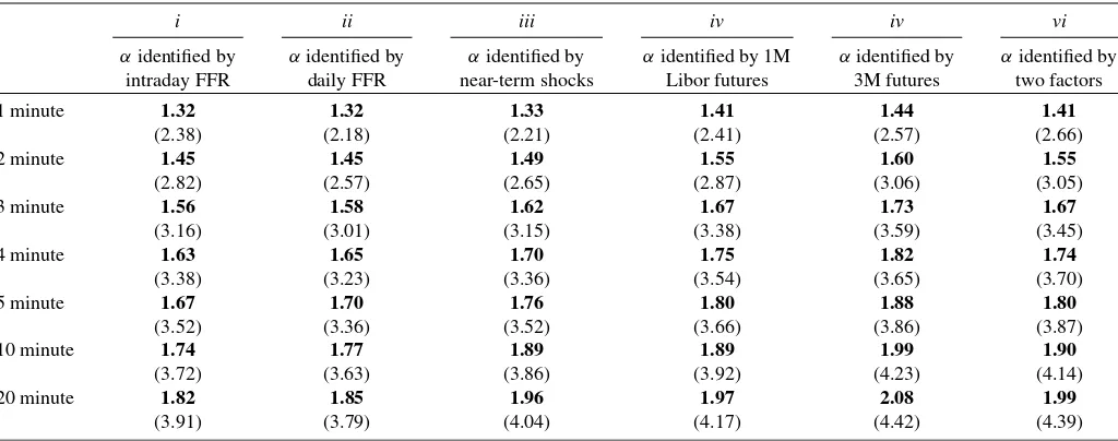
Onceαis obtained, we proceed with the second step of the identification and directly impose this estimate in the monthly VAR in order to identify the response of monetary policy to stock prices(β).We find that the response of the Fed to stock prices is positive and statistically significant. Specifically, pol-icy rates increase by 1.82 basis points in response to a 1% rise in stock prices (Table3, columni). Putting it in a more real-istic context (as in Rigobon and Sack2003), a 5% rise in the stock market tends to increase the federal funds rate by 9.1 ba-sis points. In the following section we report the policy reac-tion to stock prices across various measures of policy shocks, “broader” policy decisions that include “FOMC statements” in addition to “target rate surprises,” and sample periods. The find-ings from these robustness checks are broadly similar to our baseline estimates with the policy response remaining positive and statistically significant.
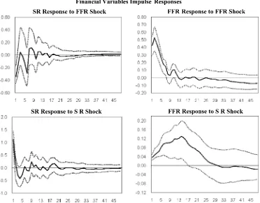
The impulse responses of financial variables to stock returns and policy shocks are shown in the top panel of Figure1. As seen, the federal funds rate rises in response to an increase in stock prices with this reaction reaching its peak 10 to 12 months after the shock and declining steadily afterwards. Stock prices fall on impact after a contractionary policy move sustaining their decline for the first two to three months. The response of macroeconomic variables to a monetary shock are broadly sim-ilar to the ones found in the literature, with economic activity, prices, business expectations (ISM), and the nonfarm payroll
declining in response to a contractionary policy shock (bottom panel of Figure1).
Though the scope of this study is to provide an identifica-tion methodology that enables the estimaidentifica-tion of contemporane-ous responses between the stock market and monetary policy, it may be of interest to evaluate if our results are realistic in an economic sense. We find that stock prices decline on average by 1.25% in response to a 25 basis points tightening in policy rates. The direction and the magnitude of this response is in line with other studies and shows that policy decisions have a sizable impact on equity markets.
The estimated reaction of the Fed to stock prices is posi-tive and significant and of the same magnitude as the one re-ported by Rigobon and Sack (2004). Through rough calcula-tions these authors evaluated the impact of stock prices on ag-gregate spending to assess whether the Fed’s reaction to the stock market is reasonable from a macroeconomic perspective. They find that a 5% rise in stock prices causes a tightening in policy rates in the range of 12 to 23 basis points and that the magnitude of this response is approximately of the same order as the one needed to eliminate the effect of the stock market on aggregate spending. Under the “stabilizing policy” of Reif-schneider, Tetlow, and Williams (1999), which reduced the im-pact of shocks on output and inflation, it appears that a perma-nent 5% increase in the stock market requires a tightening by the Fed of about 12.5 basis points. Our results fall within the range reported by these studies suggesting that the estimated policy response is consistent with that of a central bank con-cerned with developments in the stock market and their impact on the macroeconomy.
6. ROBUSTNESS
In this section several sensitivity analyses are performed to evaluate the robustness of the baseline estimates. The tests use alternative measures of policy shocks, “broader” policy deci-sions that include “FOMC statements” in addition to “interest rate surprises,” and various sample periods. The findings sug-gest that the baseline results are quite robust to these changes.
6.1 Alternative Measures of Policy Shocks
We check whether our results are robust with respect to other measures of policy shocks: (1) daily (instead of intraday) changes in spot month federal funds futures, (2) a measure that captures the “near-term path” of monetary policy, and (3) daily changes in one-month and three-month Eurodollar futures on days of policy releases. Descriptive statistics for these shocks are summarized in the right-hand side of Table1.
Estimates from daily changes in spot month federal funds futures are broadly similar to the baseline case (Table2, col-umn ii). For all event windows, stock returns decline in re-sponse to a policy tightening and this reaction increases with the size of the interval. As in the baseline case, the largest response is recorded for the 20 min interval with a surprise 1% increase in policy rates causing a decline in stock returns of 5.11%.
One potential issue with spot month futures comes from the fact that they capture the “immediate” policy surprise, which
132
Jour
nal
of
Business
&
Economic
Statistics
,
Jan
uar
y
2011
Table 1. Summary statistics: S&P500 and policy shocks
S&P500 returns Policy shocks
1 min 2 min 3 min 4 min 5 min 10 min 20 min
Intraday shocks
Daily shocks
Near-term shocks
1M Libor shocks
3M futures shocks Average All days(N=106) −0.01 0.01 0.03 0.04 0.05 0.05 0.02 −1.26 −1.20 −1.22 −1.20 −1.39 FOMC(N=102) −0.02 −0.01 −0.01 −0.01 −0.01 −0.02 −0.06 −0.41 −0.44 −0.30 −0.48 −0.66 Intermeeting(N=4) 0.29 0.66 1.02 1.29 1.51 1.82 1.94 −23.07 −21.24 −24.17 −19.37 −20.12 St. Dev. All days(N=106) 0.29 0.35 0.40 0.44 0.48 0.53 0.59 8.48 8.09 6.61 6.73 6.53 FOMC(N=102) 0.28 0.31 0.32 0.33 0.33 0.33 0.35 5.84 4.37 5.43 5.21 4.81 Intermeeting(N=4) 0.34 0.63 0.89 1.02 1.14 1.37 1.67 26.72 18.14 23.83 14.63 15.09 Max All days(N=106) 1.07 1.34 1.82 1.96 2.24 2.75 3.43 16.33 14.47 9.05 23.00 12.50 FOMC(N=102) 1.07 1.09 1.10 1.08 1.05 1.31 1.52 16.33 9.05 14.47 23.00 12.50 Intermeeting(N=4) 0.73 1.34 1.82 1.96 2.24 2.75 3.43 15.02 −0.50 10.21 1.00 2.00 Min All days(N=106) −1.02 −1.09 −1.08 −1.16 −1.21 −1.17 −0.99 −43.75 −42.50 −44.24 −33.50 −32.00 FOMC(N=102) −1.02 −1.09 −1.08 −1.16 −1.21 −1.17 −0.99 −22.55 −18.23 −19.40 −15.00 −16.00 Intermeeting(N=4) −0.11 −0.18 −0.21 −0.22 −0.19 −0.21 −0.46 −43.75 −44.24 −42.50 −33.50 −32.00 NOTE: High-frequency intervals for S&P500 and intraday shocks are computed around the time of monetary policy announcement. S&P500 returns are expressed in percent while policy shocks are expressed in basis points. Policy shocks are derived from: (1) intraday spot month federal funds futures (Intraday shocks), (2) daily spot month federal funds futures (Daily shocks), (3) intraday price changes in federal funds futures for those contracts expiring on the month of the next release (Near-term shocks), (4) daily changes in 1-Month Libor futures (1M Libor shocks), and (5) daily changes in 3-month Eurodollar futures (3M futures shocks). The sample extends from January 1994 to September 2006.
Table 2. The response of stock returns to policy actions: Estimatingα
i ii iii iv iv vi
Intraday FFR
shocks R2
Daily FFR
shocks R2
Near-term
shocks R2 1M futures R2 3M futures R2
Interest rate shocks
FOMC
statements R2 1 minute −1.48 0.19
−1.44 0.16 −1.54 0.12 −2.08 0.23 −2.31 0.27 −1.51 −0.58 0.23
(4.66) (4.35) (3.04) (4.96) (5.82) (6.43) (2.23)
2 minute −2.37 0.34
−2.38 0.31 −2.60 0.25 −3.06 0.35 −3.36 0.40 −2.49 −0.56 0.37
(6.16) (5.73) (3.76) (5.18) (7.40) (9.26) (2.06)
3 minute −3.14 0.44 −3.22 0.42 −3.51 0.33 −3.90 0.43 −4.30 0.49 −3.33 −0.52 0.47
(6.10) (5.94) (4.06) (4.71) (6.76) (8.18) (1.87)
4 minute −3.57 0.47 −3.71 0.46 −4.06 0.37 −4.42 0.46 −4.92 0.53 −3.81 −0.56 0.50
(5.81) (5.84) (4.38) (4.60) (6.64) (7.05) (2.14)
5 minute −3.89 0.48 −4.06 0.48 −4.49 0.39 −4.82 0.47 −5.38 0.55 −4.17 −0.59 0.52
(5.25) (5.34) (4.36) (4.38) (6.08) (5.93) (2.17)
10 minute −4.36 0.49 −4.58 0.49 −5.44 0.46 −5.46 0.48 −6.16 0.58 −4.82 −0.69 0.59
(4.52) (4.55) (4.83) (4.08) (5.52) (5.33) (2.18)
20 minute −4.91 0.50 −5.11 0.50 −5.92 0.44 −5.99 0.47 −6.80 0.58 −5.34 −0.80 0.62
(4.13) (4.07) (4.78) (3.98) (5.09) (4.54) (2.32)
NOTE: Estimates are obtained from high-frequency regressions around policy announcement time. Baseline results are in columni. “Interest rate shocks” and “FOMC statements” in columnviare derived from factor analysis as is Gürkaynak, Sack, and Swanson (2005). Parentheses containt-statistics from heteroskedasticity-consistent (hc3) standard errors. The sample extends from January 1994 to September 2006.
Table 3. The reaction of monetary policy to stock returns: Estimatingβ
i ii iii iv iv vi
αidentified by intraday FFR
αidentified by daily FFR
αidentified by near-term shocks
αidentified by 1M Libor futures
αidentified by 3M futures
αidentified by two factors
1 minute 1.32 1.32 1.33 1.41 1.44 1.41
(2.38) (2.18) (2.21) (2.41) (2.57) (2.66)
2 minute 1.45 1.45 1.49 1.55 1.60 1.55
(2.82) (2.57) (2.65) (2.87) (3.06) (3.05)
3 minute 1.56 1.58 1.62 1.67 1.73 1.67
(3.16) (3.01) (3.15) (3.38) (3.59) (3.45)
4 minute 1.63 1.65 1.70 1.75 1.82 1.74
(3.38) (3.23) (3.36) (3.54) (3.65) (3.70)
5 minute 1.67 1.70 1.76 1.80 1.88 1.80
(3.52) (3.36) (3.52) (3.66) (3.86) (3.87)
10 minute 1.74 1.77 1.89 1.89 1.99 1.90
(3.72) (3.63) (3.86) (3.92) (4.23) (4.14)
20 minute 1.82 1.85 1.96 1.97 2.08 1.99
(3.91) (3.79) (4.04) (4.17) (4.42) (4.39)
NOTE: Estimates are obtained by imposing the (corresponding) stock market response on a monthly VAR which includes the following variables: industrial production (IP), infla-tion (CPI), commodity prices (PCOM), nonfarm payroll (NFP), the survey of the Institute for Supply Management (ISM), S&P500 stock returns (SR), and the federal funds rate (FFR).
t-statistics (in parentheses) are computed from the recursive-design wild bootstrap of Gonçalves and Kilian (2004) based on 2000 draws. The sample extends from January 1994 to September 2006.
can be attributed to a number of factors such as the tim-ing of policy actions (advancement or postponement), the ex-pected path of near-term policy moves, or a combination of both. Clearly, announcements that cause changes in expecta-tion about the future path of monetary policy are likely to have a stronger impact on stock prices than those that reflect simply a shift in the timing of an anticipated policy action. We follow Gürkaynak, Sack, and Swanson (2007) and use intraday federal funds futures for the month of the next release to construct a measure for “near-term path” shocks. As expected, the response of stock prices to these shocks is larger than our baseline esti-mates (Table2, columniii).
The future path of monetary policy can also be captured by one-month and three-month Eurodollar futures (Cochrane and Piazzesi2002; Rigobon and Sack2004). We find that the reac-tion of stock returns is relatively larger with respect to these shocks, with a surprise 1% tightening causing a decline in stock returns of 5.9% and 6.8% for the one-month and three-month Eurodollar futures, respectively (Table 2, columns iv andv). One potential explanation for the larger response under these alternative shocks is the horizon they capture; while spot month federal funds futures deliver surprises regarding imme-diate policy moves, the nearest one-month Eurodollar futures have around one month to expiration, with the three-month fu-tures stretching further out to three months. In addition, the value of these contracts is based on the Libor rate and not the federal funds rate, so the accuracy of policy shocks they deliver depends on how closely the Libor rate follows movements in the funds rate.
Estimates ofβ associated with the various measures of pol-icy shocks are reported in Table3, columnsii–v. As seen, the response of the Fed to stock returns is positive and statistically significant and slightly larger in magnitude than our baseline re-sults. Estimates ofβappear relatively less sensitive to the mea-sure of policy surprises thanα. For example as the response of stock prices increases from 4.91% (with intradayFFRfutures)
to 6.8% (with three-month Eurodollars),βincreases from 1.82 to 2.08 basis points. It is also worth noting that the standard errors of αincrease as we move from a more accurate policy measure (intraday federal funds futures) to a less accurate one (daily changes in three-month Eurodollar futures).
6.2 Broader Policy Shocks: Incorporating FOMC Statements
So far we assumed that policy announcements are entirely captured by “interest rate shocks” as measured by changes in federal funds futures. This characterization misses an im-portant component of announcements—FOMC statements— which may effectively communicate to the public important information about the outlook for growth, inflation, and fu-ture policy moves. If FOMC announcements reveal some formation about the state of the economy that influences in-vestors’ risk aversion, they may at the same time impact federal funds futures and S&P500 futures. Stock prices incorporate the information content of FOMC releases relatively fast, and as forward-looking jump variables, the correlation between them and policy shocks may still be due to omitted factors that affect both variables.
In fact, a number of recent studies found that FOMC state-ments are as powerful as policy actions and in some instances even more powerful. Bernanke, Reinhart, and Sack (2004) and Kohn and Sack (2004) showed that FOMC statements increase the variance of asset prices relative to policy days when no statements are issued. Chirinko and Curran (2005) examined the impact of speeches, testimonies, and FOMC statements on the 30-year Treasury bond futures and concluded that FOMC statements are the most effective communicative tool. Lucca and Trebbi (2008) reported that the information content of pol-icy statements has considerable forecasting power for future short-term rates. Gürkaynak, Sack, and Swanson (GSS) (2005) showed that two factors are required to adequately capture
134 Journal of Business & Economic Statistics, January 2011
Figure 1. Impulse responses to a one-standard deviation shock are estimated assuming a recursive ordering of the macrovariables and al-lowing for contemporaneous responses between the federal funds rate and stock returns. The confidence intervals are constructed from the recursive-design wild bootstrap of Gonçalves and Kilian (2004) based on 2000 draws. The sample runs from January 1994 to September 2006.
policy actions: one factor related to the current “interest rate shocks” and the other to the “FOMC statements.” They found that FOMC statements explain around 90% of the variation in the 10-year Treasury notes.
We follow the GSS (2005) method of principle component analysis and extract the two orthogonal factors, which we la-bel “FOMC statement” and “interest rate shocks.” A high-frequency regression is then carried out by runningSP500futt,d on these two factors. Estimates indicate that the “FOMC state-ment” factor has a statistically significant impact on stock prices and the response of stock returns to “interest rate shocks” is slightly larger than in the baseline case (Table2, column vi). The fit of the models improves suggesting that a two-factor model which includes FOMC statements and interest rate sur-prises captures policy announcements more adequately.
Estimates of the Fed’s reaction to the stock market whenαis identified from the two-factor model are slightly larger than the baseline case (Table3, columnvi). As seen,β increases from 1.32 to 1.41 basis points for the 1-min interval and from 1.82 to 1.99 basis points for the 20-min interval.
6.3 Alternative Samples
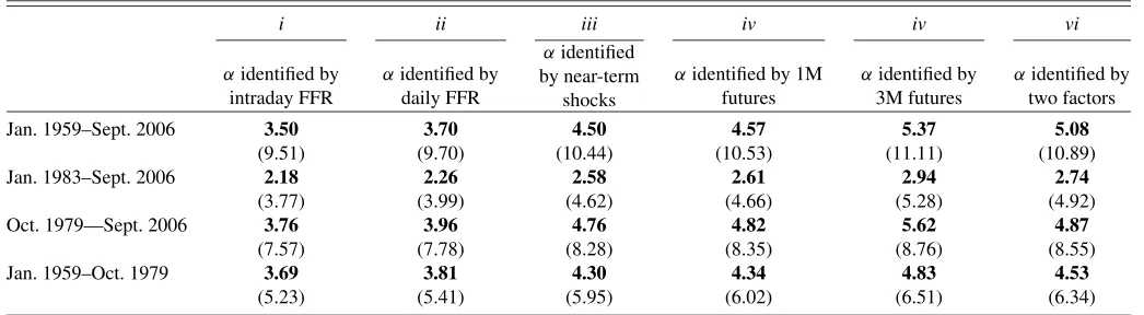
This article identifies a monetary VAR augmented with stock returns for the period from January 1994 to September 2006. We focus on these years because the high-frequency Equa-tion (4) can be carried out with precision only in the post-1994 period when the Fed has announced its decision at a prede-termined time. However, this is not a standard VAR estima-tion sample and it will be of interest to report estimates from more conventional samples. We also consider the possibility of a structural break in the conduct of monetary policy in late 1970s and early 1980s as documented by a number of studies (e.g., Bernanke and Mihov1998; Boivin and Giannoni2006).
This exercise is carried out assuming that the response of the stock market to policy shocks over all subsamples is the same as the one obtained from the 1994–2006 period. In other words, estimates ofα are still obtained from the recent high-frequency dataset, whereasβ is estimated from monthly VARs from longer periods. This approach is not new. Faust, Swan-son, and Wright (2004) also combined impulse responses esti-mated from various periods in their identification approach. The
estimation samples are: January 1959–September 2006, Janu-ary 1983–September 2006, October 1979–September 2006, and January 1959–October 1979.
Results are shown in Table4. As expected, the response of monetary policy to stock returns shows some variation over time. For the entire sample (1959–2006), we find that a 1% rise in stock returns causes a tightening of policy rates by an average of around 4.5 basis points (a 5% increase translates to a rise of 22 basis points). Results for the 1983–2006 sample are slightly larger than the baseline period with a 1% (5%) increase in stock returns causing a rise in policy rates by an average of 2.6 (14) basis points. Estimates also show that during 1979–2006 and 1959–1979 the Fed’s response to stock returns is larger than in the most recent samples. These findings suggest that the con-duct of monetary policy in recent times has changed not only toward inflation and output, but also with respect to the stock market.
7. CONCLUSION
This study develops a new identification approach to es-timate the contemporaneous responses between stock returns and policy rates in a standard monetary VAR. The method-ology combines high-frequency data from the futures market with the VAR framework to circumvent exclusion restrictions on the parameters of interest. First, intraday changes in stock prices around policy announcements are regressed on policy shocks to obtain the stock market response to policy actions. This estimate is then imposed in the monthly VAR system in order to identify the second parameter—the Fed’s reaction to stock prices. The high-frequency dataset addresses both the en-dogeneity issue (since there is no simultaneous reaction within the small time-frame around the policy release) and the omitted variable problem (by reducing the likelihood that new informa-tion is released in the market during the tight window).
The results indicate that the stock market reacts strongly and significantly to monetary policy shocks with a surprise 1% tightening in policy rates causing a decline of 4.91% in stock returns. We also estimate the Fed’s reaction to stock prices, and similar to Rigobon and Sack (2003), find this response to be
Table 4. Estimates ofβover various samples
i ii iii iv iv vi
αidentified by intraday FFR
αidentified by daily FFR
αidentified by near-term
shocks
αidentified by 1M futures
αidentified by 3M futures
αidentified by two factors
Jan. 1959–Sept. 2006 3.50 3.70 4.50 4.57 5.37 5.08
(9.51) (9.70) (10.44) (10.53) (11.11) (10.89)
Jan. 1983–Sept. 2006 2.18 2.26 2.58 2.61 2.94 2.74
(3.77) (3.99) (4.62) (4.66) (5.28) (4.92)
Oct. 1979—Sept. 2006 3.76 3.96 4.76 4.82 5.62 4.87
(7.57) (7.78) (8.28) (8.35) (8.76) (8.55)
Jan. 1959–Oct. 1979 3.69 3.81 4.30 4.34 4.83 4.53
(5.23) (5.41) (5.95) (6.02) (6.51) (6.34)
NOTE: VAR estimations are carried out assuming that the response of stock market to policy moves is the same as the one obtained from the 1994–2006 period. Estimates are identified by imposing the stock market response on monthly VARs which include the following variables: industrial production (IP), inflation (CPI), commodity prices (PCOM), nonfarm payroll (NFP), the survey of the Institute for Supply Management (ISM), S&P500 stock returns (SR), and the federal funds rate (FFR).t-statistics (in parentheses) are computed from the recursive-design wild bootstrap of Gonçalves and Kilian (2004) based on 2000 draws.
136 Journal of Business & Economic Statistics, January 2011
positive and significant. According to the estimates, a 5% in-crease in stock returns causes a rise in policy rates by 9.1 basis points suggesting that the Fed has dedicated considerable at-tention to developments in equity markets. In addition, by us-ing a different identification method, we find that the standard assumption of exclusions restriction between policy rates and stock returns is rejected.
One limitation of the proposed method comes from the fact that the time of the policy announcement can be identified with precision only in the post-1994 period. As such, analysis for longer samples can be carried out assuming that the stock market response to policy shocks has not changed over time. Nonetheless, the methodology has wide application and can be used to address identification issues arising from the endogene-ity between policy rates and other financial variables such as Treasuries, exchange rates, commodity prices, and other finan-cial instruments. One interesting generalization for future re-search will be to expand the financial block to include simul-taneously several financial variables in addition to the federal funds rate.
ACKNOWLEDGMENTS
The authors thank Jean Boivin, Jonathan Wright, Refet Gürkaynak, Serena Ng, two associate editors, and two review-ers for numerous comments and suggestions. They also thank Kenneth Kuttner, Frederic Mishkin, Brian Sack, seminar partic-ipants of the 2003 Royal Economic Society, and the 2006 Euro-pean Financial Management Association International (FMA). Part of the research was supported by the Department of Eco-nomics, Columbia University. Mira Farka acknowledges the support of California State University, Fullerton, Faculty De-velopment Research Grant Program. The opinions expressed in this article do not necessarily reflect those of the Federal Re-serve Board or of the Federal ReRe-serve System.
[Received January 2008. Revised July 2009.]
REFERENCES
Bagliano, F. C., and Favero, C. (1999), “Information From Financial Markets and VAR Measures of Monetary Policy,”European Economic Review, 43, 825–837. [127,128]
Balduzzi, P., Elton, E. J., and Green, T. C. (2001), “Economic News and Bond Prices: Evidence From the U.S. Treasury Market,”Journal of Financial and Quantitative Analysis, 36 (4), 523–541. [129]
Bentzen, E., Hansen, P., Lunde, A., and Zebedee, A. (2008), “The Greenspan Years: An Analysis of the Magnitude and Speed of the Equity Market Re-sponse to FOMC Announcements,”Financial Markets and Portfolio Man-agement, 22 (1), 3–20. [129]
Bernanke, B., and Blinder, A. S. (1992), “The Federal Funds Rate and the Chan-nels of Monetary Transmission,”American Economic Review, 82, 901–921. [128]
Bernanke, B., and Kuttner, K. (2005), “What Explains the Stock Market’s Re-action to Federal Reserve Policy?”Journal of Finance, 60, 1221–1257. [127,130,131]
Bernanke, B., and Mihov, I. (1998), “Measuring Monetary Policy,”Quarterly Journal of Economics, 113, 869–902. [128,135]
Bernanke, B., Reinhart, V., and Sack, B. (2004), “Monetary Policy Alternatives at the Zero Bound: An Empirical Assessment,”Brookings Papers on Eco-nomic Activity, 2, 1–100. [129,133]
Boivin, J., and Giannoni, M. (2006), “Has Monetary Policy Become More Ef-fective?”Review of Economics and Statistics, 88 (3), 445–462. [135]
Bomfim, A. N. (2003), “Pre-Announcement Effects, News Effects, and Volatil-ity: Monetary Policy and the Stock Market,”Journal of Banking and Fi-nance, 27, 133–151. [127]
Chirinko, R., and Curran, C. (2005), “Greenspan Shrugs: Formal Pronounce-ments, Bond Market Volatility, and Central Bank Communication,” manu-script, Emory University. [129,133]
Christiano, L. J., Eichenbaum, M., and Evans, C. L. (1996), “The Effects of Monetary Policy Shocks: Evidence From the Flow of Funds,”Review of Economics and Statistics, 78, 16–34. [128]
(1999), “Monetary Policy Shocks: What Have We Learned and to What End?” inHandbook of Macroeconomics, Vol. 1A, eds. J. Taylor and M. Woodford, Amsterdam: Elsevier, pp. 3–64. [128]
Clarida, R. H., and Gertler, M. (1997), “How the Bundesbank Conducts Mone-tary Policy,” inReducing Inflation: Motivation and Strategy, eds. C. Romer and D. Romer, Chicago: University of Chicago Press, pp. 363–406. [128] Cochrane, J. H., and Piazzesi, M. (2002), “The Fed and Interest Rates—A
High-Frequency Identification,”American Economic Review, 92 (2), 90–95. [127,
133]
Crowder, W. (2006), “The Interaction of Monetary Policy and Stock Returns,” Journal of Financial Research, 29 (4), 523–535. [127]
Ederington, L., and Lee, J. H. (1993), “How Markets Process Information: News Releases and Volatility,”Journal of Finance, 52, 1287–1321. [129] Ehrmann, M., and Fratzscher, M. (2007a), “Communication by Central Bank
Committee Members: Different Strategies, Same Effectiveness?”Journal of Money, Credit and Banking, 39 (2–3), 509–541. [129]
(2007b), “Transparency, Disclosure, and the Federal Reserve,” Inter-national Journal of Central Banking, 3 (1), 179–225. [129]
Evans, C. E., and Kuttner, K. (1998), “Can VARs Describe Monetary Policy?” inTopics in Monetary Policy Modelling, Basel: Bank for International Set-tlements. [129,130]
Fair, R. (2002), “Events That Shook the Market,”Journal of Business, 75 (4), 713–731. [127]
Faust, J., Rogers, J., Swanson, E., and Wright, J. (2003), “Identifying the Ef-fects of Monetary Policy Shocks on Exchange Rates Using High Frequency Data,”Journal of the European Economic Association, 1 (5), 1031–1057. [127]
Faust, J., Swanson, E., and Wright, J. (2004), “Identifying VARs Based on High Frequency Futures Data,”Journal of Monetary Economics, 51 (6), 1107– 1131. [127-129,135]
Fleming, M., and Remolona, E. (1997), “What Moves the Bond Market?” Eco-nomic Policy Review, Federal Reserve Bank of New York, December, 31– 50. [129]
(1999), “Price Formation and Liquidity in the U.S. Treasury Market: The Response to Public Information,”Journal of Finance, 54 (5), 1901– 1915. [129]
Gonçalves, S., and Kilian, L. (2004), “Bootstrapping Autoregressions With Conditional Heteroskedasticity of Unknown Form,”Journal of Economet-rics, 123 (1), 89–120. [128,133-135]
Gürkaynak, R., Sack, B., and Swanson, E. (2005), “Do Actions Speak Louder Than Words? The Response of Asset Prices to Monetary Policy Actions and Statements,”International Journal of Central Banking, 1, 55–93. [127,129,
131-133,135]
(2007), “Market-Based Measures of Monetary Policy Expectations,” Journal of Business & Economics Statistics, 25 (2), 201–212. [133] Jackwerth, J. C. (2000), “Recovering Risk Aversion From Option Prices and
Realized Returns,”Review of Financial Studies, 13 (2), 433–451. [130] Jackwerth, J. C., and Rubinstein, M. (1996), “Recovering Probability
Distribu-tions From Option Prices,”Journal of Finance, 51 (5), 1611–1632. [130] Jensen, G., Johnson, R., and Mercer, J. (1996), “Business Conditions, Monetary
Policy and Expected Security Returns,”Journal of Financial Economics, 40, 213–237. [127]
Kohn, D., and Sack, B. (2004), “Central Bank Talk: Does It Matter and Why?” in Macroeconomics, Monetary Policy, and Financial Stability, Ottawa: Bank of Canada. [129,133]
Krueger, J., and Kuttner, K. (1996), “The Fed Funds Futures Rate as a Predictor of Federal Reserve Policy,”Journal of Futures Markets, 16, 865–879. [129] Kuttner, K. (2001), “Monetary Policy Surprises and Interest Rates: Evidence From the Fed Funds Futures Market,”Journal of Monetary Economics, 47, 523–544. [127,130]
Lucca, D., and Trebbi, F. (2008), “Measuring Central Bank Communication: An Automated Approach With Application to FOMC Statements,” manu-script, University of Chicago. [129,133]
Piazzesi, M., and Swanson, E. (2008), “Futures Rates as Risk-Adjusted Fore-casts of Monetary Policy,”Journal of Monetary Economics, 55 (4), 677– 691. [129]
Reifschneider, D., Tetlow, R., and Williams, J. (1999), “Aggregate Distur-bances, Monetary Policy, and the Macroeconomy: The FRB/US Perspec-tive,”Federal Reserve Bulletin, 85, 1–19. [131]
Rigobon, R., and Sack, B. (2003), “Measuring the Reaction of Monetary Policy to the Stock Market,”Quarterly Journal of Economics, 118, 639–669. [126,
127,131,135]
(2004), “The Impact of Monetary Policy on Asset Prices,”Journal of Monetary Economics, 51 (8), 1553–1575. [127,129,131,133]
Rudebusch, G. D. (1998) “Do Measures of Monetary Policy in a VAR Make Sense?”International Economic Review, 39, 907–931. [129]
Sims, C. (1980), “Macroeconomics and Reality,” Econometrica, 48, 1–48. [128]
(1998), “Comment on Glenn Rudebusch’s ‘Do Measures of Monetary Policy in a VAR Make Sense?’ ”International Economic Review, 39, 933– 941. [129]
Thorbecke, W. (1997), “On Stock Market Returns and Monetary Policy,” Jour-nal of Finance, 52, 635–654. [127]
Thornton, D. L. (1998), “Tests of the Market’s Reaction to Federal Funds Rate Target Change,”Federal Reserve Bank of St. Louis Review, 80 (6), 25–36. [127]