Publication Repository ASIAPes2008

NEURAL PREDICTIVE CONTROL FOR A THREE-PHASE POWER

CONVERTER SVPWM WITH CURRENT REGULATOR

Hari Sutiksno, Mochamad Ashari, and Mauridhi Hery Purnomo Institut Teknologi Sepuluh Nopember

Kampus ITS Sukolilo Surabaya Indonesia

hari@stts.edu, ashari@ee.its.ac.id , hery@eepis-its.edu

ABSTRACT

This paper presents the application of predictive control technique using artificial neural networks for a three-phase power converter space vector PWM with current regulator. Predictive control is an algorithm to minimize the performance index of prediction model of the power converter to generate control action. The model of three-phase power converter which is used to predict the future values, is based on artificial neural network. The simulation results of the proposed method are shown by using Matlab Simulink.

KEY WORDS

Predictive Control, Power Converter, Current Regulator, Neural Networks

1. Introduction

Many three-phase rectifiers with a diode bridge rectifier circuit and capacitor on dc side are used in industrial applications. These rectifiers are very simple and low in cost. However, these rectifiers perform only unidirectional power flow and are characterized poor power factor and high harmonic line currents [1]. Therefore, a three-phase power converter space vector PWM gives a good solution for industrial application. The advantages of three-phase converters are bidirectional power flow, sinusoidal line current, possible to regulate the power factor of input line, and to stabilize the dc link voltage[1-2],[8-9],[10]. To perform a unity power factor of line current and good performance of dc link volage of a three-phase power converter, control design is required. Proportional and Integral (PI) controllers have been used to solve the problem[3]. However, it is difficult to optimise the performance of the plant. Another approach is based on the predictive control. With this strategy, plant model to predict future behaviour of plant, and an optimization algorithm is required.

As known that neural networks have been applied very sucsessfully in the identification and control of dynamic systems [4]. Multilayer perceptron is the most popular neural network that used to be applied as a

[image:1.612.328.553.264.389.2]

universal approximator for modelling of nonlinear systems and controllers.

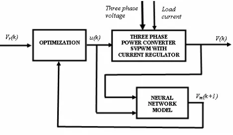
Figure 1. Three-Phase Power Converter SVPWM with Current Regulator

In this paper, it is proposed to use neural predictive control for three-phase power converter with current regulator. With this method, a neural network model is used by controller to predict the future dc voltage of converter response, so that the line currents can be controlled. An optimization algorithm computes the control signal to optimize the future plant performance. The neural network plant model is a time delayed neural network (TDNN) and trainned offline.

.

Figure 2. Neural Predictive Control of Three-Phase Converter SVPWM with Current Regulator

Proceedings of the Fourth IASTED International Conference

April 2-4, 2008 Langkawi, Malaysia

POWER AND ENERGY SYSTEMS (AsiaPES 2008)

[image:1.612.324.558.540.676.2]

⎥ ⎥ ⎥ ⎥ ⎥ ⎤ ⎦ ⎥ ⎥ ⎦ ⎢ ) ⎢ ⎢ ⎢ ⎢ ⎢ ⎣ ⎡ + ⎥ ⎥ ⎥ ⎥ ⎥ ⎥ ⎥ ⎤ ⎢ ⎢ ⎢ ⎢ ⎢ ⎢ ⎢ ⎢ ⎣ ⎡ − + − + − ⎥ ⎥ ⎥ ⎥ ⎥ ⎦ ⎤ ⎢ ⎢ ⎢ ⎢ ⎢ ⎣ ⎡ + + + + + + = ⎥ ⎥ ⎥ ⎥ ⎥ ⎦ ⎤ ⎢ ⎢ ⎢ ⎢ ⎢ ⎣ ⎡ ) , 1 ( ... ... ) 2 , 1 ( ) 1 , 1 ( 1 ( ... ) ( ) 1 ( ... ) 1 ( ) ( ) , ( .... , ( ... ... ... ... .... ... ) , 2 ( .... ) 1 , 2 ( ) , 1 ( ... ) 1 , 1 ( ) , ( .... ) 2 , ( ) 1 , ( .... ... ... ... ... ... ... ... ) , 2 ( .... ) 2 , 2 ( ) 1 , 2 ( ) , 1 ( ... ) 2 , 1 ( ) 1 , 1 ( ... ... 1 1 1 1 1 1 1 1 1 1 1 1 1 1 1 2 1 N b b b n k V k V m k u k u k u n m N w Nm w n m w m w n m w m w m N w N w N w m w w w m w w w X X X

N 1)

. .

2. Neural Predictor

In neural predictive control, neural network model of three-phase power converter will be used as a predictor. As known, that neural networks have been used very succesfully in the identification and control of dynamic systems [5]. A nonlinear system generally can be expressed in NARMAX model (Fig 3) as:

)]

(

),....

2

(

),...

1

(

),

(

),...,

2

(

),.

1

(

[

)

(

m

d

k

u

d

k

u

d

k

u

n

k

V

k

V

k

V

f

k

V

−

−

−

−

−

−

−

−

−

=

(1)

where f(.) is a nonlinear function d is dead-time

n and m is the order of the system u is the input of the system V is the output of the system

[image:2.612.359.536.54.163.2]

Figure 3. NARMAX Model

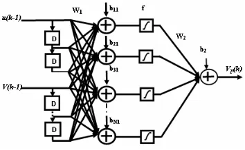
In many applications, time-delayed neural networks (TDNN) have been used to model of the plant with NARMAX. The structure of two-layer neural networks as shown in Fig.4 with sigmoid transfer functions in hidden layer, and linear transfer functions in the output layer are commonly used [6]. The number of neurons in hidden layer and output layer respectively is N and one. The size of matrices of weights W1 dan W2 respectively

is N×(m+n) and 1×N, that connect inputs to hidden layer, and connect hidden layer to the output. Then b11,…bN1

are the biases of neurons in hidden layer, and b2 is the

bias of output neuron. The output of neural networks can be expressed as follow.

[

]

2

2 ) 1 2 2 2 ) ( ... ) ( ( ) , 1 ( ... ) 2 , 1 ( ) 1 , 1 ( ) ( b X f X f X f N w w w k V N p + ⎥ ⎥ ⎥ ⎥ ⎦ ⎤ ⎢ ⎢ ⎢ ⎢ ⎣ ⎡

= (2)

where ⎥ ⎥ ⎥ ⎥ ⎥ ⎦ ⎤ ⎢ ⎢ ⎢ ⎢ ⎢ ⎣ ⎡ + ⎥ ⎥ ⎥ ⎥ ⎥ ⎥ ⎥ ⎥ ⎥ ⎦ ⎤ ⎢ ⎢ ⎢ ⎢ ⎢ ⎢ ⎢ ⎢ ⎢ ⎣ ⎡ − − − − − ⎥ ⎥ ⎥ ⎥ ⎥ ⎦ ⎤ ⎢ ⎢ ⎢ ⎢ ⎢ ⎣ ⎡ + + + + + + = ⎥ ⎥ ⎥ ⎥ ⎥ ⎦ ⎤ ⎢ ⎢ ⎢ ⎢ ⎢ ⎣ ⎡ ) , 1 ( ... ... ) 2 , 1 ( ) 1 , 1 ( ) ( ... ) 1 ( ) ( ... ) 2 ( ) 1 ( ) , ( .... ) 1 , ( ... ... ... ... ... ... ) , 2 ( .... ) 1 , 2 ( ) , 1 ( ... ) 1 , 1 ( ) , ( .... ) 2 , ( ) 1 , ( ... ... ... ... ... ... ... ... ) , 2 ( .... ) 2 , 2 ( ) 1 , 2 ( ) , 1 ( ... ) 2 , 1 ( ) 1 , 1 ( ... ... 1 1 1 1 1 1 1 1 1 1 1 1 1 1 1 2 1 N b b b n k V k V m k u k u k u n m N w Nm w n m w m w n m w m w m N w N w N w m w w w m w w w X X X N (3) and f (X) is sigmoid function.

Figure 4. The Structure of TDNN

To determine the parameters W1 , W2, b11,…bN1, and b2 , it can be done by training procedure. With this

[image:2.612.55.286.260.361.2]

procedure, training data of u(k-1) and V(k-1) is required. Fig.5 shows the training procedure for the plant. The value of u(k-1) and V(k-1) can be obtained respectively from u(k) and V(k) through a delay element. With initial weights and biases, the output of the neural network and the plant produces an error value. This value is used to correct the parameters of the network. Backpropagation is one of the training procedures in multilayer neural networks. With the new parameters, it will produce new error signal. The recursive process will continue until the minimum error is reached.

[image:2.612.326.558.355.471.2]

Figure 5. The diagram for Training of the Plant Model

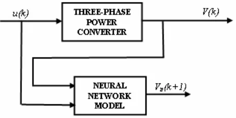
Now a neural network predictor of the plant has been obtained as shown in fig.6. With input values of u(k) dan

V(k), the neural network will produce one step prediction value of V(k+1) . It can be expressed as follow.

[

]

2

2 ) 1 2 2 2 ) ( ... ) ( ( ) , 1 ( ... ) 2 , 1 ( ) 1 , 1 ( ) 1 ( b X f X f X f N w w w k V N p + ⎥ ⎥ ⎥ ⎥ ⎦ ⎤ ⎢ ⎢ ⎢ ⎢ ⎣ ⎡ =

+ (4)

where

[image:2.612.313.558.556.704.2]

[image:3.612.56.288.103.219.2]

predictors will be used by predictive algorithm for calculating the future control signal to be applied to the power converter.

Figure 6. One Step Neural Predictor

3. Optimization Algorithm

In neural predictive control, it is expected that the time response of the output dc voltage of power converter respect to load change can be optimised. The function to be optimised is a function or error. The cost function is defined as follow:[7]

∑

₌

+

−

+

+

∑

₌

Δ

+

−

=

2 1 1 2 2

)

1

(

)]

(

)

(

[

N N i N i r p u

i

k

u

i

k

V

i

k

V

J

λ

(6)

with

Δ

u

(

k

+

i

−

1

)

=

0

,

1

≤

N

_u

<

i

≤

N

₂ (7)

where Nu is the control horizon

N1 is the minimum prediction horizon

N2is the prediction horizon

i is the order of the predictor

r is the reference trajectory λ is weight factor

The command u may be subject to amplitude constraints.

(8) 2 max

min

u

(

k

i

)

u

,

i

1

,...

N

u

≤

+

≤

=

The cost function is often used with λ=0, so J becomes:

∑

∑

+

−

+

=

+

=

= N i N N i r

p

k

i

V

k

i

e

k

i

V

J

[

(

)

(

)]

2

(

)

2

2

1

(9)

With predicted value of neural network and reference, the control action must be determined and updated based on the gradient descent method, It is simply expressed in equation:

)

(

)

(

)

1

(

k

u

J

k

u

k

u

∂

∂

−

=

+

γ

(10)

where is small number.

Based on equation (9), the term

)

(

k

u

J

∂

∂

for one-step ahead prediction can be calculated as follow.

{[ ( ) ( )] } ) ( ) ( 2 i k V i k V k u k J r

p + − +

∂ ∂ = ∂∂ (11)

)]

(

[

)

(

)]

(

)

(

[

2

)

(

k

V

k

i

V

k

i

u

k

V

k

i

J

p r p

+

∂

∂

+

−

+

=

∂

∂

(12)

where ⎥ ⎥ ⎥ ⎥ ⎥ ⎥ ⎦ ⎤ ⎢ ⎢ ⎢ ⎢ ⎢ ⎢ ⎣ ⎡ ⎥ ⎥ ⎥ ⎥ ⎥ ⎥ ⎦ ⎤ ⎢ ⎢ ⎢ ⎢ ⎢ ⎢ ⎣ ⎡ ⎥ ⎥ ⎥ ⎥ ⎥ ⎥ ⎦ ⎤ ⎢ ⎢ ⎢ ⎢ ⎢ ⎢ ⎣ ⎡ + + + = + ∂∂ ) , 1 ( .... ... ) 2 , 1 ( ) 1 , 1 ( ) ( ' 0 0 0 0 ... ... .... ... ... ... ... ... ... ... 0 0 0 ) ( ' 0 0 0 0 0 ) ( ' ) , ( .... ... ) , 2 ( ) , 1 ( )] ( [ ) ( 2 2 2 2 1 1 1 1 N w w w X f X f X f n m N w n m w n m w i k V k u N T p (13) Finally, by subtituting equation (12) and (13) into equation (10). ⎥ ⎥ ⎥ ⎥ ⎥ ⎥ ⎦ ⎤ ⎢ ⎢ ⎢ ⎢ ⎢ ⎢ ⎣ ⎡ ⎥ ⎥ ⎥ ⎥ ⎥ ⎥ ⎦ ⎤ ⎢ ⎢ ⎢ ⎢ ⎢ ⎢ ⎣ ⎡ ⎥ ⎥ ⎥ ⎥ ⎥ ⎥ ⎦ ⎤ ⎢ ⎢ ⎢ ⎢ ⎢ ⎢ ⎣ ⎡ + + + + − + − = + ) , 1 ( .... ... ) 2 , 1 ( ) 1 , 1 ( ) ( ' 0 0 0 0 ... ... .... ... ... ... ... ... ... ... 0 0 0 ) ( ' 0 0 0 0 0 ) ( ' ) , ( .... ... ) , 2 ( ) , 1 ( )] ( ) ( [ 2 ) ( ) 1 ( 2 2 2 2 1 1 1 1 N w w w X f X f X f n m N w n m w n m w i k V i k V k u k u N T r p γ (14) Now, here is the optimization algorithm:

1. Select value

2. Compute the predicted value Vp(k+1) from equation (4) and (5)

3. Compute the new control signal u(k+1)

from equation (14) 4. Return to step 2.

4.

Three-Phase Power Converter SVPWM

with Regulator

⎥ ⎥ ⎥ ⎦ ⎤

⎢ ⎢ ⎢ ⎣ ⎡

+ − =

⎥ ⎥ ⎥ ⎦ ⎤

⎢ ⎢ ⎢ ⎣ ⎡

) 3 / ) 3 / 2 cos(

2 cos(

cos

π

ωω π

ω

t v

t v

t v

v v v

m m

m

c b a

(12)

The voltages v’a, v’b dan v’c can be determined using the equation below:

⎥ ⎥ ⎥ ⎦ ⎤

⎢ ⎢ ⎢ ⎣ ⎡ + ⎥ ⎥ ⎥ ⎦ ⎤

⎢ ⎢ ⎢ ⎣ ⎡

⎥ ⎥ ⎥ ⎦ ⎤

⎢ ⎢ ⎢ ⎣ ⎡ + ⎥ ⎥ ⎥ ⎦ ⎤

⎢ ⎢ ⎢ ⎣ ⎡

⎥ ⎥ ⎥ ⎦ ⎤

⎢ ⎢ ⎢ ⎣ ⎡ = ⎥ ⎥ ⎥ ⎦ ⎤

⎢ ⎢ ⎢ ⎣ ⎡

c b a

c b a

c b a

c b a

v v v

i i i

dt d

L L L

i i i

R R R

v v v

' ' '

0 0

0 0

0 0

0 0

0 0

0 0

(13)

Then rectified current id can be obtained using this equation:

c c b b a a

d

S

i

S

i

S

i

i

=

+

+

(14)

The dc voltage VDC can be found the differential equation:

dt

dV

C

R

V

i

DC

L DC

d

=

+

(15) [image:4.612.365.516.55.180.2]

Using equations (12-15), it can be shown that dc voltage is affected by voltage source, load resistance, and control (Sa, Sb, and Sc).

Figure 7. Three-phase Power Converter Circuit Space Vector PWM is a method which is used to produce an three-phase ac voltage based on the space vector representation of voltages in the α, plane. The α,

components can be obtained using Clarke transformation as follow:

ref c b a

v v v

v v

⎥ ⎥ ⎥ ⎦ ⎤

⎢ ⎢ ⎢ ⎣ ⎡ ⎥⎦ ⎤ ⎢⎣

⎡

− − − =

⎥ ⎦ ⎤ ⎢ ⎣ ⎡

866 . 0 866 . 0 0

5 . 0 5 . 0 1 3 2

β

[image:4.612.324.556.322.427.2]

α (14)

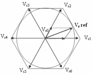
Fig. 8 shows 8 space vectors in according to 8 switching positions of inverter, V’ is the phase-to-center voltage which is obtained by proper selection of adjacent vectors Vs1 and Vs2.

Figure 8. Space Vector Voltage The reference space vector V’ is given by

T T Vs T Vs

V_'= 1 1+ 2 2 ₍₁₅₎

where T1, T2 are the intervals of application of vector Vs1 and Vs2 respectively, and zero vectors V0 (Sa=0, Sb=0 and

Sc=0) and V7 (Sa=1, Sb=1 and Sc=1) are selected for T0. They can be calculated using these equations:

)]

3

cos(

)

3

sin(

[

1

π

π

β

α

m

v

m

v

V

T

T

_{s s}

DC

s

−

=

(16)

)] 3

) 1 ( cos( )

3 ) 1 ( sin( [

2

π π

β

α − + −

−

= v m v m

V T

T s s

DC

s ₍₁₇₎

and

2 1

0

T

T

T

T

=

s

−

−

(18)

The space-vector PWM current regulator is accomplished by estimating the appropriate duty cycles for the α- space vectors adjacent to the reference vector in such a way that the line current is driven to the reference value at the end of period of time. In the case of steady-state operation, this is equivalent to calculating a reference voltage vector that accomplishes the deadbeat control and calculating the duty cycles for the appropriate states using space-vector PWM. Considering the voltage-source converter power circuit shown in Fig. 1, if Ts is

assumed to be small in comparison with the period of the source voltage (V ), then V can be assumed constant over the period Ts: Let tn denote the time at the beginning of one Ts period. Then, the change in line current over one period (neglecting the source resistance) is

s n s n n

ac n

T

t

I

T

t

I

L

t

I

L

t

V

t

V

(

)

(

)

=

(

+

)

−

(

)

Δ

Δ

=

−

(19)

where Vref is the average value of the ac-side rectifier

voltage over Ts.

[image:4.612.56.286.382.480.2]

)

(

)

(

t

n

T

s

KV

t

n

T

s

I

+

=

+

(20)

Substituting I(tn+Ts) from equation (20) into equation(19) and rearranging, the ac-side rectifier voltage is [9]:

)

(

)

(

)

(

)

2

1

(

)

(

n

s s n s n s n

ac

I

t

T

L

T

t

I

T

KL

t

V

T

KL

t

V

=

−

−

−

−

(21)

Using equation (20), input line current of the power converter can be regulated by means of the input K.

5. Simulation results

The predictive control of three-phase power converter SVPWM with current regulator has been simulated using Matlab Simulink R14 (Matlab 7.0). In this simulation, it is asumed that the data of three-phase power converter given below:

• Phase Voltage Source 100 Volt (max)

• Output Voltage (DC) = 300 volt

• Voltage Frequency = 50 Hz

• Input Inductance L = 3mH

• DC Link Capacitor C = 2200uF

• Switching Frequency 5kHz

• Full Load Resistance RL = 35 Ohm

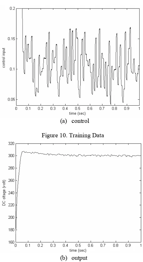
[image:5.612.325.553.47.465.2]

To compute the parameters of network, the training data will be required. This training data can be obtained using the method shown in fig.9.

Figure 9. Diagram for Training Data Provider

[image:5.612.327.553.55.255.2]

(a) control Figure 10. Training Data

[image:5.612.56.292.460.640.2]

(b) output Figure 10. Training Data

In this case, the three-phase power converter must be operated in close loop system using PI controller. The training data represents relationship between input control and output voltage (dc voltage) with load changes as its parameter. Form the results of simulation as shown in fig.10, neural network can be trained using Levenberg and Marquard method. Neural model of the plant has been established succesfully using TDNN with 2 inputs, 8 neurons hidden layer, and single output.

[image:6.612.55.290.52.450.2] [image:6.612.55.283.484.668.2]

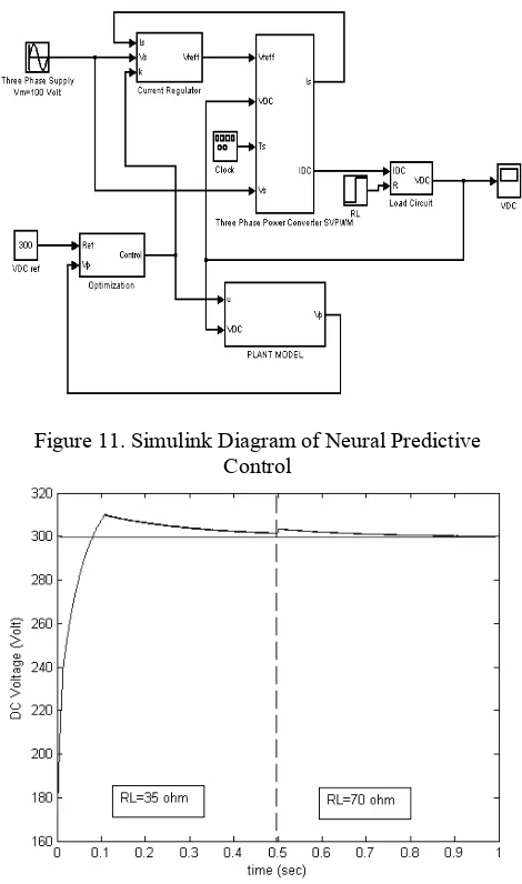
Figure 11. Simulink Diagram of Neural Predictive Control

Figure 12. Time Response of DC Voltage respect to the load change

Figure 13. Line Current (line A)

6. Conclusion

With the use of current regulator in three-phase power

currents with a dc value (not a sinusoidal function). Therefore, the neural model of the plant can be built simply using time-delayed neural network (TDNN).

From the simulations results, Neural Predictive Control for three-phase power converter SVPWM provides a good dynamic of controlled voltage, line currents in phase with line voltage, and gives low harmonic distortion.

References

[1] P. Antoniewicz and M.P. Kazmierkowski, Predictive direct Power Control of Three-phase Boost Rectifier,

Bulletin of the Polish Academy of Sciences, Vol 54, No.3, 2006, 287-292.

[2] S.Y. Ron Hui, Henry Shu-Hung Chung, A Bidirectional AC-DC Power Converter with Power Correction, IEEE Transactions on Power Electronics,

Vol.15, No.5, 2000, 942-949.

[3] Vitor Fernao Pires and Jose Fernando A. Silva, Single-Stage Three-Phase Buck-Boost Type AC-DC Converter With High Power Factor, IEEE Transactions on Power Electronics, Vol.16, No.6, November 2001, 784-793.

[4] Orlando de Jesus and M. Hagan, Backpropagation Algorithms for a Broad Class of Dynamic Networks,

IEEE Transactions on Neural Networks, Vol.18, No.1, January 2007, 14-27

[5] Shi Hong-li , Cai Yuan-li and Qiu Zu-lian, System Identification based on NARMAX Model using Hopfield Networks, Journal of Shanghai University, Vol 10 no.4 June, 2006, 238-243.

[6] Bimal K.Bose, Neural Network Applications in Power Electronics and Motor Drives-An Introduction and Perspective, IEEE Transactions on Power Electronics, Vol.54, No.1, Februari 2007, 14-33

[7] Leizer Schnitman and Adhemar de Barros Fontes, The Basic of Neural Predictive Control, Proceeding of the

7th Mediterranian Conference on Control and

Automation(MED99) Haifa, Israel, June 28-30, 1999. [8] Yi-Hwa Liu, Chern-Lin Chen and Rong-Jie Tiu, A Novel Space Vector Current Regulation Scheme for Field-Oriented-Controlled Induction Motor Drive, Trans IE, Vol. 45, no.5, 1998.

[9] Suttichai Saetieo, and David A.Torey, Fuzzy Logic Control of a Space Vector PWM Current Regulator for Three-Phase Power Converters, IEEE Transactions on Power Electronics, Vol13, No.3, 1998, 419-426