Mothers’ Time Choices
Caregiving, Leisure, Home Production, and
Paid Work
Jean Kimmel
Rachel Connelly
a b s t r a c t
Using data from the 2003 and 2004 American Time Use Survey, we study the role that socioeconomic factors play in mothers’ time choices. We estimate a four-equation system in which the dependent variables are the minutes used in home production, active leisure, market work, and child caregiving. Our results show that mothers’ caregiving time increases with the number of children, decreases with age of the child, and increases with the price of child care. We also find a substantial positive wage elasticity for caregiving time, while both leisure and home production time declines with increased wages.
I. Introduction
The last half of the twentieth century was a period of dramatic trans-formation in the role that women play in society, highlighted most clearly by the rapid rise in paid employment of mothers with young children. Currently, about 60 percent of mothers with children younger than six participate in the paid work force. As mothers have increased their paid work efforts, conflicts between employ-ment and family responsibilities have grown, leading researchers to explore more
Jean Kimmel is an associate professor of economics at Western Michigan University and Research Fellow of IZA, Bonn. Rachel Connelly is professor of economics at Bowdoin College. The authors thank the W.E. Upjohn Institute for Employment Research for financial support for this research. They also thank Dawit Senbet and Fei Tan for research assistance and Erdal Tekin, Dorinda Allard, and two anonymous reviewers for providing feedback that substantially improved the paper. Finally, they thank their children for enlightening them regarding the distinction between the process and outcome utility components of caregiving time. Earlier drafts of this manuscript were presented at the November 2005 SEA meeting, December 2005 ATUS Early Results Conference, and the January 2006 ASSA meeting. The data used in this article can be obtained beginning January 2008 through December 2010 from Rachel Connelly, Department of Economics, Bowdoin College, Brunswick ME 04011,
connelly@bowdoin.edu.
[Submitted March 2006; accepted September 2006]
ISSN 022-166X E-ISSN 1548-8004Ó2007 by the Board of Regents of the University of Wisconsin System
fully the role that caregiving responsibilities play in mothers’ time choices and the effects that these choices may be expected to have on their children.
Our paper relies on the recently released American Time Use Survey (ATUS) data to describe the time-use choices of mothers in the United States. Using these data, we describe how mothers allocate time to four aggregated categories of time: home pro-duction, caregiving time, leisure, and paid market work, with a focus on identifying differential responses to demographics and prices for these different time uses. Our four time-use categories, which expands the analysis beyond the traditional three time-use categories of paid work, leisure and home production by explicitly separat-ing caregivseparat-ing time from home production, permits us to identify the factors relevant to caregiving time choices. Additionally, this more detailed stratification enables us to gain a better understanding of how mothers’ caregiving time choices compare to their choices regarding other unpaid uses of time, household production and leisure time. If caregiving time responds differently in any substantive way to economic and demographic factors, then aggregating caregiving time into household production or leisure time might yield mistaken empirical conclusions.
The first goal of the paper is to describe mothers’ time responsiveness to economic factors. Specifically, we estimate market wage and childcare price elasticities for each of four general categories of time utilization, thereby providing for both abso-lute and relative interpretations. We find that all four time uses of mothers in the United States are sensitive to wages and childcare time is sensitive to childcare prices of preschoolers but less so to childcare prices for school-age children. Most interest-ingly, we find that higher-wage mothers devote more time to caregiving both on weekdays and weekend days, ceteris paribus. Additionally, paid work time on week-days also responds positively to higher wages, while leisure time and home produc-tion weekday time are reduced by higher wages.1 On weekends, only leisure time and childcare time are impacted by higher wages, with leisure time decreased and childcare increased for higher-wage mothers.
The second motivation for this research is to gain a better understanding of the importance that marital status, race, and other demographic factors play in time choices, once economic factors are controlled, and to determine whether these factors affect competing time choices differently. We expect to find that single mothers make time-use decisions very differently from their married counterparts, in part due to the lesser availability of adults in the household to engage in home production, resulting in a greater need to purchase products in the market. With regard to race, previous research on the use of nonparental childcare has revealed different childcare utiliza-tion patterns by race, and we wonder whether these differences carry over to mater-nal time use as well. Difference in time use by race may help explain differences observed in other policy-relevant variables such as differences by race in the gender wage gap or in wealth acquisition. Examining the role of race in four different time uses will allow us to identify the different roles that race could play in these very different activities.
Finally, our third goal with this research is reflected in methodological improve-ments, most importantly our implementation of a structural model of time choice in which the correlation across time choices is incorporated into the econometric
methodology. Additionally, we implement a Tobit model to permit incorporation of individuals observed allocating their time into fewer than our four categories (for ex-ample, mothers who do not work for pay on diary day or who have no home produc-tion minutes on diary day).
The rest of the paper is as follows: Section II reviews the economic literature on time allocation from the Robbins labor/leisure tradeoff model through the work of Becker and Gronau, concluding with the empirical literature that looks explicitly at childcare time. Section III outlines a behavioral model of four distinct time uses for mothers of young children, while Section IV discusses the ATUS data and our esti-mation strategy. Section V presents our results and Section VI summarizes the findings.
II. Time Allocation Models and Mothers’ Time Use
Economists have long understood that the standard Robbins (1930) labor/leisure model is inadequate for understanding the time-allocation process of mothers. The microeconomic theory underlying the labor/leisure framework posits that paid work yields no direct utility thus paid work enhances the worker’s utility only via the goods purchased with the earned income (outcome utility). In addition, the theory posits that all time devoted to leisure produces utility directly (process utility). The very foundation of the theory of neoclassical labor supply relies on the credibility of this stratification of time into time-yielding process utility and time-yielding outcome utility. This theoretical underpinning, while perhaps a reason-able stretch for men, is not appropriate for women who still do the majority of house-work and childcare even as their paid house-work hours have increased.2The New Home Economics models of the early 1960s acknowledged that a substantial portion of time not spent in paid employment is home production time, not leisure.3Becker’s (1965) methodology omits all time categorizations and focuses on the production of final consumption commodities, but this approach has been difficult to implement empirically due to difficulty identifying the final commodities. Since then, alternative approaches have focused on expanding the traditional two-dimensional time alloca-tion model to three or more uses of time with the hope of disentangling activities that are unpaid but produce substantial outcome utility (and can be traded across mem-bers of a household ) from the leisure time category.
Gronau (1977) and Graham and Green (1984) stratified time outside the labor mar-ket into home production and pure leisure. Gronau (1977) establishes two criteria for aggregating time uses and concludes that leisure time and home production time should not be combined. Gronau writes: ‘‘From the theoretical point of view, the jus-tification of aggregating leisure and work at home into one entity, nonmarket time (or home time) can rest on two assumptions: (a) the two elements react similarly to changes in the socioeconomic environment and therefore nothing is gained by study-ing them separately; and (b) the two elements satisfy the condition of a composite
2. For a discussion of the difficulty associated with stratifying time use into separate categories to distin-guish those generating outcome utility from those generating process utility see Juster (1985), Dow and Juster (1985), and Oi (1992).
input, that is, their relative price is constant and there is no interest in investigating the composition of the aggregate since it has no bearing on production and the price of the output’’ (p. 1100).4
But in fact, Gronau’s two criteria explain why, particularly for mothers, his three uses of time are still not enough. In his model, unpaid ‘‘home work’’ is defined as time spent producing a good that is a perfect substitute for one that also could be purchased in the market. In addition to home-produced goods and market-produced goods being indistinguishable, the home-production process in Gronau’s model pro-vides no utility per se. However, home-produced childcare (henceforth referred to as parental childcare or caregiving) is usually considered an imperfect substitute for market childcare in the production of child services and certainly most parents re-ceive utility from some of the time they spend on caregiving.5For studying the time use of mothers, the best solution to this problem is to expand the Gronau trinity into a model with five aggregated uses of time: (paid) market work, (unpaid) home work, child care, leisure and other.6The other category includes sleep, personal care time, education, and job-seeking endeavors and can be loosely thought of as personal in-vestment time.
This expanded Gronau model is, in our view, a credible means of assigning activ-ities into composite categories that produces a manageable number of categories while disentangling a complex group of unpaid caregiving activities we refer to as caregiving from leisure and household production. But it must be made clear that any attempt to take an extensive list of human activities and categorize the activities into five distinctly different groups with total homogeneity within groups is impos-sible.7Thus, the categorization we choose is ad hoc at best, but does seem sensible in light of Gronau’s two criteria and yields a number of time uses that can be modeled with appropriate econometric sophistication.8 Additionally, isolating caregiving-related activities into their own category permits us to compare caregiving time choices to other unpaid time choices.
What is the existing state of knowledge regarding the determinants of mothers’ child caregiving time? The bulk of the previous literature that examines caregiving time focuses on couples, often dual earner households. Kooreman and Kapteyn (1987) looked exclusively at married couples and found that higher wages of the father increased the time their wives spent in child care, but that women’s own wages affected neither her childcare time nor her husband’s childcare time. Nock and
4. Note that neither of Gronau’s two criteria rely on the distinction between process and outcome utility. 5. See, for example, Aguiar and Hurst (2006).
6. Van den Brink, Maassen, and Groot (1997) use four categories of time use, leisure, home production, childcare, and employment. Kooreman and Kapteyn’s (1987) model includes eight categories.
7. In fact, we do not estimate the determinants of the ‘‘other’’ time category as it is far too heterogenous in terms of activities included.
8. Note that empirical application of any aggregated time-use model requires something akin to a leap of faith because it is not possible to distinguish time uses that provide process utility from those providing only outcome utility. Many activities that would typically be categorized as household production or care-giving may produce process utility (as does paid work). For example, time spent preparing a meal may be a chore for some, while others may enjoy the process of creating a meal. Our four time aggregates, while limited by the same problems associated with distinguishing process utility from outcome utility that have always hindered neoclassical time-use models, is a best attempt to categorize comparable activities into dis-tinct groups that respond in similar ways to economic and demographic factors.
Kingston (1988) found that mother’s employment reduced their childcare time, but that the reductions were mostly in secondary activities with children.9Using data from the Netherlands for married mothers currently employed, Van den Brink, Maassen, and Groot (1997) found no effect of husband’s earnings on the time allocation of his wife in employment, home production, or child care. Closest to our research is the recent paper by Hallberg and Klevmarken (2003). They examine the determinants of parents’ time allocated to childcare in Sweden and their structural model incorpo-rates instruments for both parents’ wages and parents’ employment time. They find that own wages do not affect childcare time of their sample of Swedish parents.
Studies using more recent time diary data from the United States have found that employment hours are a predictor of hours spent with children; however, mothers ap-pear to shield their children from the full impact of their employment by cutting back on personal time, sleep, leisure, and home production rather than reducing child care. Thus, there is some evidence that caregiving time is treated differently than either home production or leisure.10The differences by gender in the time trend data de-scribed by Sayer (2005) provide more support for this notion. Sayer notes that over time, men and women have adjusted their out of market time substantially, concen-trated mainly in their movement from unpaid home production into family time. Thus, the disaggregation of unpaid activities is becoming more important over time.11 Kalenkoski, Ribar, and Stratton (2005a) use British data to estimate a reduced form model, in which wages are not included directly. They find that women with an ad-vanced degree spend more time on primary child care, secondary child care, and market work. What they are spending less time on is not clear since these are the only three uses of time included in their analysis. Kalenkoski, Ribar, and Stratton (2005b) show a sim-ilar result for U.S. mothers using the ATUS, namely that mothers with a bachelor’s degree or a graduate degree spend more time on primary childcare and in market employment.
III. Underlying Behavioral Model
The behavioral model underlying our empirical specification is the standard neoclassical individual-based utility maximizing problem in which mother’s utility is expressed as a function of leisure,tL, child services, CS, and aggregated
adult consumption of final goods and services excluding child services,G.
maxU¼UðtL;CS;GÞ
ð1Þ
9. Both papers use data from U.S time diaries from the 1975-81 Time Use Longitudinal Panel. 10. For examples of this research, see Howie et al. (2006), Bianchi et al. (2005), Reimers (2002), Sandberg and Hofferth (2001), Bianchi (2000), and Bryant and Zick (1996).
11. Sayer (2005) and Craig (2006) both note that while men are adjusting their unpaid time in response to mothers’ increased paid work time, the result thus far is not one of gender equity in all time uses. Craig expresses the concern that this the movement of women into the paid work force is only half a ‘‘revolution,’’ and has resulted in an increased total work load for women. One positive outcome of the time-use evolution (as noted by Sayer et al. 2004) is that parental time investments in their children has increased, contrary to much media reporting.
Adult consumption goods,G, are home produced with a combination of house-hold production time, thp, and purchased intermediate goods;G¼G(thp,X;u).uis an
efficiency parameter which is affected by differences in ability, but also by differen-ces in personal investment including sleep time and educational endeavors. Child services,CS, are also home produced, but with a combination of the mother’s care-giving time,tmcc,nonmaternal childcare time (including that provided by the father),
tcc, and market-produced child goods,CX;CS¼CS(tmcc,tcc,CX;f). Likeu,fis an
efficiency parameter. On the constraint side of the model, there is a mother’s time constraint, Equation 2, and a budget constraint, Equation 3.
T¼tem+thp+tmcc+tL+ts
ð2Þ
PXX+Pcctcc+PCXCX¼wtem+V
ð3Þ
The mother’s total time can be divided into market-paid time,tem, home-production
time,thp, caregiving time,tmcc, leisure,tL,and investment time,ts.12In addition,
im-plicitly there is a child’s time constraint in that parents with young children (which we define as parents with children younger than 13) must have someone watching their children at all times.
CT¼tmcc+tcc+tscc
ð4Þ
CTis the total amount of time available to children. We have already definedtmccas
maternal childcare time andtccas nonmaternal time, both of which contribute to
increased levels of child services. The final term,tscc, is secondary childcare time
in which children are being supervised but not actively engaged. For the sake of modeling ease, this secondary care time is assumed to not contribute to child ser-vices and to be provided without opportunity cost by the mother or without money cost by anyone other than the mother. If we think of tsccas including sleep time
thenCT¼T.
The above three constraints result in three distinct costs of a mother’s time. First, there is the cost of time in the labor market,w2Pcc, if the alternative to employment
is primary care of one’s own children.13The second cost of time is when the mother is engaged in leisure or home-production activities while children are not present be-cause the children are actively engaged by an alternative caregiver. The opportunity cost of that activity’s time is the price of earnings forgone plus the price of nonpar-ental child care,w+Pcc, At other times, when children are being supervised in the
background, when children are in public school, or when children are old enough for self care, the opportunity cost of that activity’s time is simply the wage, w. Since the cost of time is sometimes the wage, sometimes the wage plus the price of child care,
12. Note that this theoretical model reflects a Gronau like assumption that only leisure yields process utility. Caregiving time, household production time, and market work yield outcome utility only. 13. See Connelly (1992) and Ribar (1992, 1995) for models of nonmaternal childcare that derive thew-Pcc
cost of time.
and sometimes the wage minus the price of child care, the wage and the price of childcare must appear separately in any estimation model.14
The behavioral model described above results in time-demand functions for the five different uses of time, as well as the more standard consumption good demand functions forGandCX. Equation 5 presents a general functional representation of the time-demand functions.
tj¼fðw;Pcc;VjZ;H;DÞ for j¼em;hp;mcc;L;s
ð5Þ
Time use is related to factors reflecting the value of time, including the wage and the hourly prices of nonparental childcare for women with preschool-aged children and school-aged children, the amount of nonlabor income available to the mother, pref-erences, and institutional structure, all of which are expected to be related to personal characteristics of the mother,Z, characteristics of the household in which she resides,
H, and characteristics of the diary day,D.
IV. Data and Estimation Strategy
A. The ATUSAs described above, our primary goal in this paper is to examine the determinants of time spent in four activities: leisure, child care, home production, and paid employ-ment for mothers, with a focus on caregiving. We exclude the ‘‘other’’ category as too heterogeneous to aggregate. We aim to contrast the factors important in caregiv-ing choices with other unpaid activity, namely household production and leisure. We admit that in both our theoretical discussions and empirical implementation we have largely ignored the role played by spouses or partners. The ATUS collected one time diary per household. Because one’s spouse’s time data are unavailable, we make the assumption that the only role of the spouse is in his production of earned income which is treated as unearned income by his wife. Time diary designs in other coun-tries allow a more nuanced look across couple time tradeoffs.
We draw our data from the 2003 and 2004 samples of the American Time Use Sur-vey. Our estimating sample is comprised of female ATUS diary respondents between the ages of 18 and 65 who have children younger than13 living in the household, are not part of a multifamily household, and are not currently in the active duty military, in school, or unemployed. These criteria, in addition to requiring each observation to have information on the husband’s wage if married with spouse present, leads to a sample size of 4,552 mothers.15 Because weekdays and weekends represent very
14. Kimmel (1998) provides empirical justification for including separate measures for the wage and the price of care in employment equations.
15. Only women who are mothers are included in our empirical analyses. This sample stratification is based on the outcome of motherhood, which is modeled within the choice framework by economists. We do not address this endogeneity because the complexity of our model renders such econometric exten-sions infeasible and such methodologies require data typically unavailable (e.g., variables thought to ex-plain motherhood that do not also exex-plain time use). However, our focus here just on mothers makes this endogeneity correction less important. It would be more important in a time-use comparison between mothers and nonmothers.
different time-use patterns for many families and because the ATUS oversamples end days, we separate the data throughout the analysis into weekends and week-days.16Ultimately, we have usable time diary information from 2,156 women for weekdays and 2,396 for weekend days.
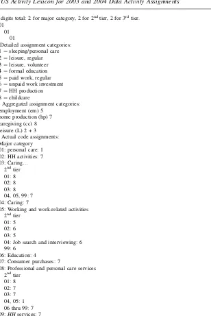
As described earlier, we categorized the time activities included in the ATUS data into four categories for estimation purposes, plus an excluded fifth category.17 Ap-pendix Table 1 records the full set of decisions we made in assigning the six-digit time categories provided by the ATUS into our five category framework. In terms of the caregiving time, we mainly use time categorized by the ATUS as ‘‘Caring and Helping Household Children,’’ but have added time spent engaging nonparental caregivers and transportation time to nonparental care arrangements to the main cat-egory of child caregiving time. Similarly, telephone and travel time related to secur-ing professional help in housework was added to home-production time.
The delineation of leisure time requires some elaboration. According to the New Home Economic models, all time that produces utility directly ought to be consid-ered leisure time. Application of this theory to an actual list of human activities is not straightforward. One example of an activity that can be problematic to categorize is sleeping. While some fraction of sleeping can be considered an activity producing process utility, a sizable portion is a necessity for human existence and would best be categorized as a variation of human capital investment. (See, for example, Biddle and Hamermesh 1990). Aguiar and Hurst (2006) discuss in detail the difficulties inherent in ‘‘defining’’ leisure and examine leisure trends using four different definitions of leisure time. They too express concern with the investment component and necessity of sleep. To address this concern, we omit time spent sleeping or engaging in per-sonal care from our aggregate measure of leisure, resulting in a measure that can best be thought of as active leisure.
The group category of caregiving also can be difficult to conceptualize, particu-larly when one considers the distinction between process utility and outcome utility. Only a portion of mothers’ time with their children is exclusively devoted to caregiv-ing. This time would include feeding, bathing, playing games, talking, and reading to children. We expect that some of this time provides process utility but surely not all of the time on all of the days. Yet, these are the sorts of activities that the ATUS picks up in primary caregiving time, time when the respondent herself categorizes the time as primarily childcare activities. Other activities in which children are involved are
16. In fact, weekend employment typically is referred to as nonstandard employment. Also, note that we include weekday holidays in the weekend sample so the sample is really weekends and holidays. We do this because there are very few weekday holidays in the data and but those holidays look very different from weekdays in time-use patterns. Kalenkoski, Ribar and Stratton (2005b) divide their data in the same way. 17. This fifth time category is all other time and includes time spent sleeping, in personal care, time spent in educational pursuits, unpaid time that contributes to success in one’s current employment, and job search time. It is not essential for our estimation procedure that all 24 hours in a day be accounted for in these four time uses, and in fact, we account for considerably fewer than 24 hours. The correlation among the equa-tions is addressed through cross-equation covariances, not in cross-equation coefficient restricequa-tions as would be necessary if we were accounting for all time within a 24-hour period. Solberg and Wong (1992) and Kim and Zepeda (2004) do account for all time while Kalenkoski, Ribar, and Stratton (2005a, 2005b) do not. Concern for the hetergeneity of the fifth category and the complexity of the estima-tion model even without trying to account for cross-equaestima-tion restricestima-tions led us to estimate the Tobit equiv-alent of Seemingly Unrelated Regressions (see Prowse 2004).
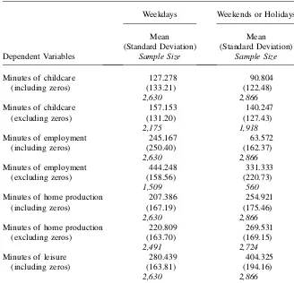
more likely categorized as time spent with children, such as the always-pleasurable trip to the supermarket with squabbling children in tow, which is likely to have been categorized as home-production time.18Again some of this time may produce pro-cess utility, though most would be expected to produce outcome utility (healthy chil-dren). Finally, there is passive care that the ATUS collects as time when children are recorded as ‘‘in the room’’ which excludes time when all household children are sleeping and the time when the respondent is sleeping. Passive care includes time at home when one is listening for children calling or overseeing children engaged in play. Folbre et al. (2005, p. 374) encourage moving beyond the simple categori-zation of time into activities to incorporate even broader notions of responsibilities or constraints. Thus, their description of passive care would be broader than that available in the ATUS, and would include being responsible for sleeping children, even if the parents are sleeping too. Unfortunately, the data produced by existing time-use surveys do not reflect the broad characterization suggested by Folbre et al.19 Table 1 presents the average minutes spent in the four time categories for the mothers in our sample. Looking at Table 1, we see substantial differences between weekdays and weekends in the time spent in our four categories. Leisure and home-production times are higher on weekends while the opposite is true for em-ployment and childcare time. It is a bit surprising that less time is spent in active caregiving on the weekend than weekday as the number of hours of employment also is substantially lower on the weekend. These differences provide suggestive evidence that time spent in childcare is distinct from home production and leisure. Addition-ally, the dramatic differences in time use between weekdays and weekends serves to support our decision to estimate our time-use models separately for those two diary day groups.
Table 1 also shows substantial differences in the means of childcare, home produc-tion, and employment time depending on whether the zeroes are included. The sub-stantial number of respondents with zero time use in these categories means our estimation strategy should explicitly take account of the left censoring of the time responses at zero. On the other hand, very few in the sample have zero minutes of active leisure, and no one has a full day of leisure so we need not be concerned about censoring of the leisure-time equation.20
Further descriptive information is presented in Table 2. The top half of the table shows the expected relationship between age of the youngest child and the number of minutes spent on child care. Married mothers whose youngest child is younger than five spend 198 minutes in active childcare on a weekday and 145 minutes on a weekend day. The number of minutes decreases substantially when the youngest
18. Kalenkoski, Ribar, and Stratton (2005a) examine childcare time reported both as primary and second-ary time usages.
19. ATUS permits respondents to record childcare as a secondary activity (having children ‘‘in your care’’) when it is not the reported primary activity. Two recent papers by Kalenkoski, Ribar, and Stratton (2005a, 2005b) address the childcare measurement issue by focusing on different measures of nonprimary caregiv-ing. Kalenkoski, Ribar, and Stratton (2005a) use data from the United Kingdom to examine factors impor-tant to primary and secondary childcare (as well as market) time use, while Kalenkoski, Ribar, and Stratton (2005b) use data from both the United Kingdom and the United States and a broader definition of secondary care that includes all time spent with children not reported as the primary activity.
20. Fifteen respondents have zero minutes of active leisure on weekday and five report zero minutes of active leisure on weekends.
child is elementary-school aged, to 75 minutes on weekdays, and 46 minutes on a weekend day. The pattern is similar for unmarried mothers though the number of minutes is less, particularly for unmarried mothers with preschool children.21 Mar-ried women also spent more time on home production than unmarMar-ried women, sug-gesting that a husband’s presence increases requisite work in the home or that unmarried mothers ‘‘contract out’’ more of the home production. Standards may be higher in married households and there is another person in the house for whom to produce goods. This finding is consistent with previous research into gender
Table 1
Average Minutes Spent per Day on Leisure, Childcare, Home Production, and Employment for Women with Children Younger than 13
Weekdays Weekends or Holidays
Note: Each cell contains the variable mean, standard deviation, and number of observations
21. We define those who are married with spouse present as married and all other mothers are defined as not married. Thus, unmarried mothers with partners residing in the household are treated the same as mothers without partners. This is a weakness we aim to address in future research.
Table 2
Average Minutes Of Time Used by Age of the Youngest Child, Marital Status, Wage Category for both Weekdays and Weekend Days
Married Spouse Present Not Married Spouse Present
Youngest Child: 6 to 12
Youngest Child: 0 to 5
Youngest Child: 6 to 12
Youngest Child: 0 to 5
Weekday
Minutes in paid work 284.69 188.98 314.55 179.46 Minutes in childcare 75.44 197.72 67.79 174.48 Minutes in home production 224.10 227.75 164.00 157.50 Minutes in leisure 422.47 383.18 287.60 389.10 Weekend
Minutes in paid work 68.79 40.71 86.71 80.13 Minutes in childcare 46.13 145.21 44.91 121.74 Minutes in home production 280.25 252.08 251.23 202.39 Minutes in leisure 422.47 383.18 423.20 389.10
(continued)
Kimmel
and
Connelly
Table 2 (continued)
Married Spouse Present Not Married Spouse Present
Low Wage Mid Wage High Wage Low Wage Mid Wage High Wage
Weekday
Minutes in paid work 320.54 368.21 369.81 287.37 254.06 400.06 Minutes in childcare 85.75 98.59 111.46 124.49 96.72 86.88 Minutes in home production 171.56 168.01 161.46 150.61 142.26 126.14 Minutes in leisure 254.14 233.24 248.47 253.88 243.10 249.51 Weekend
Minutes in paid work 128.80 79.68 69.50 128.95 130.77 86.21 Minutes in childcare 59.85 74.42 95.25 61.76 76.06 73.09 Minutes in home production 254.14 276.82 275.18 221.75 229.88 242.93 Minutes in leisure 360.46 382.95 393.87 374.66 374.22 412.61
Note: Data from 2003 and 2004 ATUS. Reported results are weighted to reflect population averages. The Mid-wage category was calculated the mean predicted wage plus or minus one standard deviation from the mean.
654
The
Journal
of
Human
differences in home-production time, including that of South and Spitze (1994) and Stratton (2003).
The bottom half of Table 2 shows the distribution of average time use by marital status and wage rate categories. The middle wage category is defined as the approx-imate mean wage in the full sample ($10) plus and minus one standard deviation ($2.00). Thus, a low wage is a wage less than $8 an hour and a high wage is a wage greater than $12 an hour.22As expected, women with high wages are employed in the labor market on the diary day for more minutes but only on weekdays. On week-ends, higher wages are correlated with fewer minutes of employment time. For the most part, unmarried mothers are employed more minutes than married women, es-pecially on weekdays for unmarried mothers in the highest wage category.
Table 2 also shows that childcare time, like employment time, increases with mar-ried women’s wages, but the same is not true on weekdays for unmarmar-ried mothers. Those unmarried mothers with the highest wages devote less time for childcare than middle wage unmarried mothers and less still than low-wage unmarried mothers. For married women, the result is consistent with Bryant and Zick’s (1996) finding that more highly educated mothers spend more time in direct child care.
B. Empirical Model
The evidence presented in Table 2 is merely a cross-tabulation. A fuller understand-ing of the relationship among time use, marital status, age of children, and wages requires a multivariate analysis. Our basic estimation model is a system of four linear time-use equations based on the time-demand equations shown in Equation 5. The estimation version of Equation 5 can be characterized as:
tj ¼b0j+b#jX+ej for j¼em;hp;mcc;L
ð6Þ
wheretj* is the latent number of minutes a mother would choose to spend in activity j. The actual observed minutes,tjwill equal zero whentj* is less than zero. In our
sample, active leisure was so seldom zero that we can ignore the censoring problem for the leisure equation.
A Tobit model is used often to account for situations like Equation 6 if one is will-ing to assume that theej’s are normally distributed. In our case, in addition to ac-counting for the lower limit constraint, we also must account for the fact that four observed time uses come from the same sample respondent. More time used in one activity likely means less time used in some other activity. We assume that theejterms are correlated across equations in the following way:
eL
This situation is analogous to Seemingly Unrelated Regression except we must use a nonlinear estimation technique to account for the lower limit constraints in three out
22. The wage measure used here is actually a wage measure generated from preliminary estimation. This predicted wage is created using a standard two-step Heckman correction. For details, see Section IV4.
of the four equations. Accounting for both the constraint at zero minutes and the cor-relation among error terms, leads to our choice to estimate a system of four corre-lated equations, three of which are estimated as Tobit equations.23
TheX’s of Equation 6 include standard demographic characteristics of the mother,
Zi,characteristics of the household,Hi,characteristics of the diary day,Di, and three
predicted price of time measures. We discuss each set of variables briefly in turn. The vectorZiincludes variables such as age, education, urban/rural residence, Southern/
non-Southern residence, Nonwhite/White, and Hispanic/non-Hispanic. These varia-bles may reflect differences in time preferences and also, in the case of residence var-iables, differences in the price of commodities and structural demands on one’s time. For example, urban dwellers may spend more or less time commuting to work and traveling related to shopping. Southern dwellers may have more yard work or other differences in time demands.
We do not have strong theoretical predictions concerning the pattern of the effect of these demographic variables, nor are there many previous empirical studies of caregiving versus home-production time to inform our expectations. Studies of non-parental childcare use have shown that nonwhite use more relative care than whites, so that we could hypothesize that nonwhite mothers will spent less time in caregiv-ing (Capizzano et al. 2000 and NCES 2004).24Finally, studies of hours of house-work have reported a substantial drop in time spent on househouse-work. If standards of housecleaning have declined, we might expect an age-cohort effect such that older women spend more time on home production than younger women. (Bianchi 2000).
The variables included in characteristics of the household,H, include Married Spouse Present/ Not Married or No Spouse Present, Husband’s Earnings (if Married Spouse Present, zero otherwise), the presence of other adults in the household (per-sons older than 17 who are not the woman or her spouse), and five counts of the num-ber of children in the household aged zero to two, three to five, six to nine, ten to 12, and 13 to 17. Other studies simply have included the total number of children and the age of the youngest child, but we expect that children of different ages contribute differently to the demands on mothers’ time. Certainly, Table 2 shows substantial time-use differences by age of the youngest child. Studies of the effect of the pres-ence of children on mother’s employment have found differpres-ences between having a zero to two-year-old versus having a three to five-year-old. One reason for this dif-ference is that many families view preschool as an educational investment in their children, not just as supervised time that facilitates women’s employment, but still, utilizing preschool does free up the mother’s time while the children are at school. Six- to nine-year-olds are in school much of the day but they are usually not left alone before and after school, while ten- to 12-year-olds are left alone often. Teen-agers bring their own set of time and money demands which may affect mothers’
23. Our estimation procedure is very similar to that used by Kalenkoski, Ribar, and Stratton (2005a, 2005b) except we have four uses of time and they model three. Our fourth equation, for leisure time, is estimated via OLS. The estimation was done as a system of equations using the statistical software package aML. 24. Even if nonwhite mothers use more relative care it might not affect their own caregiving time if relative care simply substitutes for other employment enabling childcare such as center or family daycare home-based care. On the other hand, a relative who is available for employment enabling care also may provide home-production-enabling or leisure-enabling care.
employment. (This has sometimes been shown for school-aged children as well.) Teenagers also could contribute time (at least potentially) to household childcare and home production, freeing up maternal time for employment and leisure.25Connelly, DeGraff, and Levison (1996) found strong evidence of this in urban Brazil, but the results for the United States have been weaker. However, sibling care may be used to facilitate mothers’ leisure or home-production activities rather than employment, which would not show up in employment-based studies. The presence of other adults in the household may affect mothers’ time use if household members truly behave as a cohesive unit, but even in that case, the direction of the effect is not clear. A co-residing adult could contribute income to the household, thus freeing up the mother to do more of the home production and caregiving, or could contribute childcare and home production time, freeing up the mother for more employment time. The core-siding adult also may increase home-production time, especially if the corecore-siding adult is an elderly relative who requires care.26
Economic theory does not provide us with strong predictions about the effect of marriage and husband’s earnings on time-use decision-making. The presence of the spouse should reduce childcare and home-production time to the extent that he participates in these tasks, but the demand for home-production tasks also increases. We saw in Table 2 that the presence of the spouse is correlated with greater home-production time. In addition, controlling for husband’s earnings, married women have higher rates of employment, which would lead to increased employment time and reduced child caregiving time. The higher rates of employment could be due to positive assortative mating or the husband facilitating maternal paid employment, even if he is not directly providing child care. His presence may provide another set of relatives to draw on for emergency care or his time simply may add flexibility to the woman’s time choices, such that employment is easier to sustain. Assuming hus-band employment time is exogeneous (which is, in the dawn of the 21stcentury still not a bad assumption), husband’s earnings play the role of nonlabor income in our model. Higher levels of nonlabor income are expected to reduce all ‘‘work’’ time (employment and home production), and should increase leisure time, but the effect on caregiving depends on the weighting of the ‘‘work’’ versus the ‘‘consumption’’ components of childcare time. However, higher nonlabor income also may mean a bigger house or more ‘‘stuff’’ to take care of, so even the effect on home production is ambiguous.
We control for the season of the year the diary information was collected with a dichotomous variable indicating if the diary month was June, July, or August. In pre-liminary work, we included a dummy for each season but found that the only signif-icant differences in time use were observed in summer. We expect that summer matters for mothers of young children because of school vacation and changes in the activities and even sleep patterns of children with the increased daylight hours and warm temperatures.
The last three regressors represent components of the price of time. The price of time is expected to affect all uses of time and so is included as a determinant of
25. Mothers who have only teenagers at home are excluded from this analysis so the teenagers in our sam-ple are all potential babysitters as they all have younger (12 years of age or younger) siblings. 26. We have included care of other household members in the home-production category.
leisure, caregiving, home production, and employment time. As discussed in Section III, women with children younger than13 sometimes face an additional cost of their time beyond their hourly wage which is represented by the price of child care. For very young children, supervision is necessary at all times so that an hour of mother’s time in the labor market means she receives her wage, but she may have to pay for an hour of child care. On the other hand, an hour of childcare provided by the mother means that she does not have to pay for childcare that hour. Leisure and home pro-duction are sometimes engaged in simultaneously with supervisory child care. For these uses of time, the price of childcare is not relevant, but there are uses of adult leisure time for which nonparental childcare is used and the same can be expected for some home-production time (try painting the bedroom with an awake two-year-old at home). Thus, the price of childcare is included in all four time-use equations.
C. Estimations to Produce Instruments for Economic Factors
All the variables used as determinants of time use described above except for the three time cost variables come directly from the ATUS. The three price of time variables, on the other hand, are predicted values obtained from initial stage estimation. The pre-dicted wage is obtained, as is typical, by estimating a sample-selection-corrected wage equation using ATUS data. We would have liked to generate the price of nonparental childcare the same way but the ATUS data do not include childcare expenditure infor-mation.27Instead, to model childcare costs we used the fourth wave of the 2001 Panel of the Survey of Income and Program Participation, which was administered between September and December 2002. Employed women with children younger than five were asked about their expenditure on childcare for their youngest child. In addition, employed women with children between the ages of six and 14 were asked about their expenditure on childcare for their youngest child in that age range. We eliminated those whose youngest child was 13 or 14 and those who were either currently in the military, in school, or unemployed. We used the resulting sample to estimate the price of child-care for children age five or under and separately for children between the ages of six and 12. We could have then averaged the zero- to five-year-old price of childcare and the six- to 12-year-old price of childcare, but we have chosen to keep them separate since the availability of five or six hours of school time which doubles as nonparental childcare time makes childcare for six- to 12-year-olds very different from that for chil-dren five and under. The procedure we used to estimate the hourly price of childcare is a standard bivariate selection correction model described by Tunali (1986) and used by Connelly and Kimmel (2003a, 2003b). Using this procedure, we predicted the weekly expenditure on childcare correcting for the self-selection of being both employed and paying for care. The childcare price equation is
Pcci¼a0+aZi+u1l1i+u2l2i+ui
ð7Þ
wherel1andl2correct for the sample selection of only employed mothers who are paying for care being included in the estimating sample. Having estimated the model
27. Another option is to use exogenous local childcare price measures but those data are unavailable nationally for our time period.
using SIPP data, we then used the dot product of the predicted coefficientsaand the
Zi’s from the mothers in the ATUS sample. This dot product can be interpreted as
the predicted weekly expenditures, unconditional on paying of care and being employed.28
D. Identification
Estimating multistep models such as these requires strict attention to equation iden-tification. We confront these issues at two levels. At the first level, the wage and the two prices of childcare are estimated in two-step procedures, first estimating selection terms and then estimating the wage or price of childcare with the sample-selection term included as an explanatory variable.29While theoretically one can estimate this type of sample-selection model identifying off of the functional form only, most researchers feel more comfortable basing identification on exclusions, that is, variables that are thought to affect the dichotomous choice that are not expected to affect the wage or the price of child care. In our case, we include a number of po-tential identifiers in the dichotomous-choice equations. Variables included in the re-duced form employment and pay for care equations that are not included in the price of childcare equation include second order terms of age and education, an education-age interaction term, a dichotomous variable indicating the presence of other adults in the household beyond the spouse (PRESENCE), the maximum TANF award in the state of residence for a family of three (TANFAMT), and their state’s per capita med-icaid budget (STMEDICAID). SIPP respondents are not asked for childcare expendi-ture if relatives were used so that if expendiexpendi-tures are offered, it does not include any money paid to relatives. Thus,PRESENCEis expected to be a good candidate for an identifier, strongly predicting the probability of paying for childcare, but not affect-ing the amount paid once caregivers other than other household adults are used.
In first stage estimations of both the price of childcare for children zero to five and the price of childcare for children aged six to 12, several of the identifying variables are significant. In the case of price of childcare for zero- to five-year-olds, age-squared and the education-age interaction term are significant in both the probability of paying for care and the probability of being employed, whilePRESENCEis sig-nificant in the probability of paying for care. In the case of price of childcare for six- to 12-year-olds, age-squared was a significant predictor of the probablity of employment and education-squared, PRESENCE, and TANFAMTwere significant predictors of the probability of paying for care.
Variables included in the reduced-form employment equation that are not included in the wage equation include all the variables listed above plus husband’s earnings, a dichotomous variable denoting married spouse present, the number of children in five age categories, and six state-level childcare variables: a dichotomous variable if the state provides a tax credit for childcare expenses (STCCCREDIT), a dichotomous variable if the state requires that childcare teachers have a minimum level of training
28. As is well known, incorporating generated regressors in this way produces biased standard errors. Due to the complexity of our model, we have not corrected the estimated standard errors for this bias. 29. Results for the three models used to estimate the predicted components of the price of time are avail-able in a data appendix from the authors.
(MINTRAIN), a dichotomous variable if the state requirement for child/teacher ratio for infants is four to one or better (INFANTSZ), a dichotomous variable if the state requirement for child/teacher ratio for four-year-olds is ten to one or better (4YROLDSZ), the number of licensed childcare centers per child younger than five in the state (LICCENTERS), and the number of licensed daycare homes per child younger than five in the state (LICHOMES). Estimation shows that education squared, husband’s earnings, and the number of children aged zero to two, three to five, and six to nine are all significant predictors of employment.
The second level of concern with identification comes from the use of these three generated regressors in our four time-use equations. For the predicted natural log wage, the preliminary estimation involves a sample-selected wage regression that includes one variable not also appearing in the time-use equation. Our identifying variables at this stage are state-level regressors thought to affect the individual’s wage, but not their time allocation choices: a dummy variable indicating the existence of a state minimum wage that is higher than the federal minimum wage (STATEMIN), the state’s unem-ployment rate (UNEMPLR), and the state’s female labor force participation rate (STLFPR). Additionally, we use age-squared as another potential identifier. All four potential identifiers for the wage equation are significant in the wage-equation estima-tion. TheF-test of the wage-equation estimation also is significant at the 0.01 level, in-dicating that all the included variables contribute to the prediction of wage levels. For the two childcare price measures, identification requires that at least one variable ap-pear in the childcare price equations that does not also apap-pear in the time-use equation. These identifying variables are the six variables listed above that reflect state childcare regulations and the three state labor market variables just listed that serve as identifiers of the wage equation. TheLICCENTERSvariable which is the number of licensed childcare centers per child younger than five in the state is a significant predictor of both prices of the child care.MINTRAIN, a dichotomous variable if the state requires that childcare teachers have a minimum level of training, also was found to be a significant predictor of the price of childcare for children zero to five. In addition, bothF-tests were found to be significant at the 0.01 level.
E. Descriptive Statistics for All Regressors
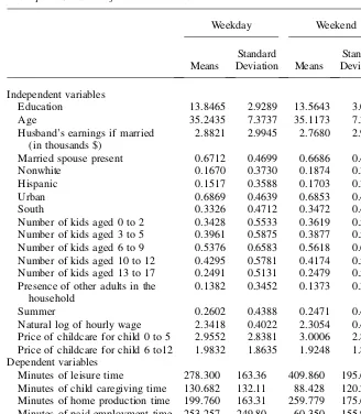
Table 3 presents the descriptive statistics for all the right-hand side variables for both the weekday sample and the weekend sample. Note that there are 2,156 observations in the weekday diary sample and 2,396 in the weekend sample. The wage is pre-sented in its natural logarithm form. The husband’s earnings is reported in thousands of dollars. There are no substantive differences in these variables by weekday/week-end status so we describe the means for the weekday sample only. Sixty-seven per-cent of the women in the sample are married and they are on average, nearly 35 years old with 14 years of education. In 2003, there was an oversampling of minority pop-ulations, as reflected in the high percentages nonwhite and Hispanic (16.7 percent and 15.2 percent respectively). Sixty-nine percent reside in urban areas and fully one-third reside in the south. Fourteen percent of the women report having another adult (other than a husband) residing in the same house. Finally, approximately one-fourth of the diaries were recorded in the summer reflecting the fact that ATUS data is collected evenly throughout the calendar year.
V. Results
We will not discuss results from instrumenting regressions in text ex-cept for the discussion of the significance of the identifiers that we have already pro-vided in the previous section. Full tables of instrumenting regressions are available from the authors. The results are very similar to those reported in (Connelly and Kimmel 2003a, 2003b) which used SIPP data from the early 1990s. For our jointly
Table 3
Descriptive Statistics of Model Variables
Weekday Weekend
Means
Standard
Deviation Means
Standard Deviation
Independent variables
Education 13.8465 2.9289 13.5643 3.0684
Age 35.2435 7.3737 35.1173 7.3555
Husband’s earnings if married (in thousands $)
2.8821 2.9945 2.7680 2.9555
Married spouse present 0.6712 0.4699 0.6686 0.4708
Nonwhite 0.1670 0.3730 0.1874 0.3903
Hispanic 0.1517 0.3588 0.1703 0.3760
Urban 0.6869 0.4639 0.6853 0.4645
South 0.3326 0.4712 0.3472 0.4762
Number of kids aged 0 to 2 0.3428 0.5533 0.3619 0.5630
Number of kids aged 3 to 5 0.3961 0.5875 0.3877 0.5599
Number of kids aged 6 to 9 0.5376 0.6583 0.5618 0.6801
Number of kids aged 10 to 12 0.4295 0.5781 0.4174 0.5803
Number of kids aged 13 to 17 0.2491 0.5131 0.2479 0.5260
Presence of other adults in the household
0.1382 0.3452 0.1373 0.3442
Summer 0.2602 0.4388 0.2471 0.4314
Natural log of hourly wage 2.3418 0.4022 2.3054 0.4273
Price of childcare for child 0 to 5 2.9552 2.8381 3.0006 2.8404
Price of childcare for child 6 to12 1.9832 1.8635 1.9248 1.8654
Dependent variables
Minutes of leisure time 278.300 163.36 409.860 195.65
Minutes of child caregiving time 130.682 132.11 88.428 120.26
Minutes of home production time 199.760 163.31 259.779 175.65
Minutes of paid employment time 253.257 249.80 60.350 155.97
Number of observations 2,156 2,396
Note: Unweighted sample, 2003 and 2004 combined, prices of childcare and wages are predicted from preliminary regression analysis.
estimated four time-use equations, we will discuss first the weekday results then the weekend results. Within each, we discuss results by variable category, and for the price of time variables, we include a discussion of elasticities.
A. Results for Weekday Observations
1. Demographic variables
Table 4 presents the estimated marginal effects of minutes spent in the four time uses on weekdays while Table 5 presents the results for weekends.30A quick glance down the columns confirms the cross-tabulation findings of Table 2 that childcare is dis-tinct from both leisure and home production. For example, the effect of age on time use (recall we are controlling for wage levels and number of children) is to increase home production and decrease employment time, but has no effect on childcare time or leisure. Being married also increases home-production time, but decreases child-care time and has no effect on leisure. Having controlled for marital status, increased husband’s earnings, which we argued could be thought of as nonlabor income, was predicted to decrease all ‘‘work’’ activities. However, home-production time, child-care time, and active leisure time on weekdays are all significantly increased by in-creased husband’s earnings while employment time is dein-creased. However, these results are consistent with the hypothesis discussed above that higher income fami-lies demand higher levels (either quality or quantity) of active childcare and home-production time and these higher levels require more time inputs.
Race, ethnicity, and location of residence all have some significant effects on mother’s time use. Nonwhites spend 15 minutes fewer on childcare time and 22 minutes fewer on home production than whites, everything else held constant. This maybe related to their increased use of relatives as caregivers. (Capizzano et al. 2000 and NCES 2004) His-panic mothers have 44 fewer minutes of leisure time. Urban dwellers have fewer em-ployment hours on weekdays and more leisure time while mothers in the southern part of the United States have less leisure time than those in the rest of the United States.
2. Household variables
One key set of variables that we are interested in are the household configuration var-iables, identified in Equation 6 asHi.As we expected, having very young children
(aged zero to two) increases women’s time in childcare on weekdays substantially. Each additional child in that age range results in 80 extra minutes of childcare time. That extra time per infant comes mostly from reduced employment time (70 minutes), but leisure time also is reduced by 25 minutes while home-production time is increased by 26 minutes. Older children (aged three to five, six to nine, and ten to 12) have very similar effects on women’s time, but the effects are substantially smaller in magnitude except for home-production time, which is constant across
30. The values in Table 4a and b represent the derivative oftjwith respect to the independent variable. To obtain the derivative oftjwe multiplied the estimated coefficients,b^j, by the probability of a nonzero
out-come. The marginal effects for leisure time use are the same as the estimated coefficients since none of the respondents reported zero hours of leisure so the equation is estimated via OLS. These probabilities were evaluated at the mean for all regressors. Appendix Tables 2 and 3 report the estimated coefficients and the standard errors on which Tables 4 and 5 are based.
Table 4
Marginal Effects of Determinants of Minutes Spent in Leisure, Childcare, Home Production, and Employment on Weekdays
Leisure Childcare Home Production Employment
Constant 439.4903*** 222.0218 147.3203*** 269.8198
Education 13.0114*** 24.9928 20.5631 26.4230
Age 1.2037 20.0722 3.6527*** 23.6201***
Husband’s earnings if married 5.9477*** 4.7878*** 6.6700*** 217.6408*** Married spouse present 212.3864 223.8672*** 23.4174** 36.2282** Nonwhite 14.1703 214.8408** 222.4255** 0.9829 Hispanic 243.9022*** 22.5102 11.4811 20.8476
Urban 15.9404* 7.1125 1.4185 241.8116***
South 218.0707** 7.5062 29.2894 16.2221
Number of kids aged 0 to 2 225.4392** 80.1256*** 26.2197*** 269.8574***
Number of kids aged 3 to 5 2.7702 28.1157*** 16.3076* 229.3285** Number of kids aged 6 to 9 0.3099 22.9401*** 20.1500*** 227.3929*** Number of kids aged 10 to 12 22.6773 12.7691*** 27.1969*** 219.4092* Number of kids aged 13 to 17 22.4415 20.4437 13.8782** 29.3123
(continued)
Kimmel
and
Connelly
Table 4 (continued)
Leisure Childcare Home Production Employment
Presence of other adult inhh 1.1066 26.7721 13.3390 229.3536*
Summer 12.6641 231.7880*** 7.8386 2.0005
Natural log of hourly wage 2165.6010*** 62.2430** 271.7931** 209.5590*** Price of childcare for child 0 to 5 22.2878 6.0730*** 1.8526 25.7434 Price of childcare for child 6 to12 1.4508 21.3862 22.6749 3.1452 Cross-equation correlations
Rho: leisure/childcare 20.1574*** Rho: leisure/employment 20.4742***
Rho: childcare/employment 20.2894*** Rho: leisure/home production 20.0148 Rho: childcare/home production 0.0364 Rho: employment/home production 20.6075***
Note: Data from 2003 and 2004 ATUS, Husband’s Earnings are in thousands of dollars, prices of childcare and wages are predicted from preliminary regression analysis. Significance: *10 percent, **5 percent, ***1 percent.
664
The
Journal
of
Human
Table 5
Marginal Effects of Determinants of Minutes Spent in Leisure, Childcare, Home Production, and Employment on Weekends
Leisure Childcare Home Production Employment
Constant 462.8083*** 2107.1041*** 146.2859*** 289.7651*** Education 11.6544** 24.7687* 21.9214 1.6036
Age 0.3274 0.1073 2.5911*** 0.0260
Husband’s earnings if married 0.0882 1.9387* 1.3085 22.0103 Married spouse present 4.6266 27.2938 14.6225 23.0168
Nonwhite 12.2872 29.1224* 223.5542** 213.4909** Hispanic 215.8090 2.4514 20.2984 23.6313
Urban 21.0202** 20.6323 24.5745 22.8442
South 10.2817 0.4153 27.3340 1.3623
Number of kids aged 0 to 2 229.3549** 58.0459*** 22.6638 215.5785** Number of kids aged 3 to 5 220.8147 18.0242*** 1.7497 2.7910 Number of kids aged 6 to 9 211.8620* 13.5260*** 8.2686 24.1315 Number of kids aged 10 to 12 217.9904** 28.1259* 19.5356*** 21.5292
(continued)
Kimmel
and
Connelly
Table 5 (continued)
Leisure Childcare Home Production Employment
Number of kids aged 13 to 17 4.2859 26.8526 7.3363 6.4037 Presence of other adult in hh 230.8597*** 9.4008 28.0590 17.0387**
Summer 19.4379** 28.7726* 4.4149 25.3668 Natural log of hourly wage 2100.5444** 83.4965*** 23.0591 6.6137
Price of childcare for child 0 to 5 0.0065 2.8187* 2.1908 0.1687 Price of childcare for child 6 to12 7.1482** 26.0663*** 2.9067 0.2380 Cross-equation correlations
Rho: leisure/childcare 20.2524*** Rho: leisure/employment 20.4274*** Rho: childcare/employment 20.0648* Rho: leisure/home production 20.4475***
Rho: childcare/home production 20.1133*** Rho: employment/home production 20.2431***
Note: Data from 2003 and 2004 ATUS, Husband’s Earnings are in thousands of dollars, prices of childcare and wages are predicted from preliminary regression ana-lysis.Significance: *10 percent, **5 percent, ***1 percent.
666
The
Journal
of
Human
children’s age groups. For older children, leisure time is no longer reduced sig-nificantly. Teenagers seem to have no effect on mothers’ time during the week except in terms of home-production time, which is increased by 14 minutes a weekday.
As we discussed above, married mothers spend less time in childcare and leisure and more time in household production. Finally, the last household characteristic var-iable is the presence of other adults in the household. The presence of these adults does not affect childcare, home production, or leisure, but does decrease employment by 29 minutes. This result contrasts with Kalenkoski, Ribar, and Stratton (2005b) who found negative effects of other adults present on mothers’ weekday childcare, both primary and passive.
3. Diary Day Characteristics
The season in which the diary was collected affects time use, with summer weekdays being a time of less childcare time (32 minutes). It is extremely interesting that sum-mer should affect childcare time in this way since school is not providing the five to six hours of childcare that it does during the school year for school aged children. It appears that the self-reported childcare time is more rigidly tied to regular weekday routines and that summer loosens our routines, reducing the time that is categorized as childcare time. Kalenkoski, Ribar, and Stratton (2005b), using the same data, also find that summer substantially reduces women’s weekday primary childcare time. They find that women’s weekday passive childcare time is increased in the summer by about as many minutes as primary childcare time is reduced.
4. Price of Time Variables
In the standard labor/leisure model, an increase in the wage is expected to increase hours worked and decrease leisure, assuming that the substitution effect is greater than the income effect, as is typically the case for women. In other words, the push toward increased work due to the rising opportunity cost of leisure dominates the push toward increased leisure demand due to rising income. This is exactly what we find using our measures of employment and leisure time. With a wage increase, em-ployment minutes are increased while leisure time was decreased . Home-production time also is decreased by an increase in wages, as would be predicted in the Gronau model, as women substitute time in the market for home-production time. But if childcare time had been included in leisure or in home production, we would have found much smaller effects. Indeed, an increase in the wage increases childcare time by more than an hour. This result is very robust to specification changes and is true whether we include mothers with children less than 18 years of age, or as reported here, mothers with children younger than 13. We believe that this result comes from a strong income effect on demand for high quality of childcare and that high-quality childcare takes more maternal time rather than more purchased child resources. Ap-parently, this strong income effect is driving mothers to substitute time away from home production toward more caregiving time, likely enhancing the investment as-pect of child care. Note that this contradicts the findings of Hallberg and Klevmarken (2003) and Kooreman and Kapteyn (1987) who found that own wages do not affect childcare time, but these studies were done using data from very different cultural settings and time periods.
A higher price of childcare for children aged zero to five increases the amount of maternal childcare time as one would expect from an own price effect. Recall that the price of childcare for children zero to five is only applied to those women with children in that age range. The price of childcare for older children did not have a significant effect on mothers’ time choices. This suggests that there exists more flex-ibility in choices of childcare options for school-aged children, including possibly free after-school care and self-care.
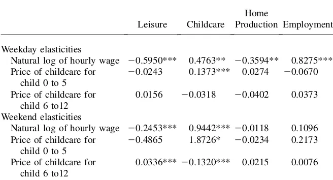
Table 6 presents the elasticities evaluated at the means implied by the marginal effects in Table 4. All the elasticities are less than one in absolute value, implying that each of these four uses of time, leisure, home production, and market work are relatively insen-sitive to the price of time. Employment time responsiveness to wage changes is poinsen-sitive, with an elasticity substantially greater in absolute value than home production, caregiv-ing, or leisure time.31A 10 percent increase in the wage leads to an 8 percent increase in time spent in weekday employment and a 5 percent increase in time spent in weekday child care. Leisure declines by 7 percent and home production declines by approximately 3.5 percent. The elasticity of caregiving time with respect to the price of childcare for pre-school children is much smaller in absolute value than the wage effect. A 10 percent in-crease in the price of childcare is predicted to reduce mother’s weekday employment hours by 1.2 percent and increase childcare time by 1.3 percent.
Table 6
Estimated Elasticities of Price of Time on Time Use in Four Activities
Leisure Childcare
Home
Production Employment
Weekday elasticities
Natural log of hourly wage 20.5950*** 0.4763** 20.3594** 0.8275*** Price of childcare for
child 0 to 5
20.0243 0.1373*** 0.0274 20.0670
Price of childcare for child 6 to12
0.0156 20.0318 20.0402 0.0373
Weekend elasticities
Natural log of hourly wage 20.2453*** 0.9442***20.0118 0.1096 Price of childcare for
child 0 to 5
20.4865 1.8726* 20.0234 0.2173
Price of childcare for child 6 to12
0.0336*** 20.1320*** 0.0215 0.0076
Note: Calculated from marginal effects from Table 4 and 5 and sample means. Significance: *10 percent, **5 percent, ***1 percent of the underlying coefficients
31. This estimate of the wage elasticity of paid work hours is within the range of results found by other researchers. See, for example, Mroz (1987) and Kaufman and Hotchkiss (2003).