More at Work?
A Nonparametric Assessment
Daniel J. Henderson
Alexandre Olbrecht
Solomon W. Polachek
a b s t r a c t
This paper investigates how students’ collegiate athletic participation affects their subsequent labor market success. By using newly developed techniques in nonparametric regression, it shows that on average former college ath-letes earn a wage premium. However, the premium is not uniform, but skewed so that more than half the athletes actually earn less than nonath-letes. Further, the premium is not uniform across occupations. Athletes earn more in the fields of business, military, and manual labor, but surprisingly, athletes are more likely to become high school teachers, jobs that pay rela-tively lower wages to athletes.
Daniel J. Henderson is an assistant professor of economics at the State University of New York at Binghamton (Binghamton University). Alexandre Olbrecht is an assistant professor of economics at the Anisfield School of Business at Ramapo College of New Jersey. Solomon W. Polachek is a distinguished professor of economics at the State University of New York at Binghamton (Binghamton University). The authors would like to thank Cliff Kern, Jeff Racine and two anonymous referees for useful comments on the subject matter of this paper. The research on this project has also benefited from participants of the Binghamton University Departmental Seminar Series, Ramapo College of New Jersey Departmental Seminar as well as participants at the 2004 Annual Meeting of the Canadian Economic Association, Toronto. Finally, the authors thank James Long for providing the data necessary for this project along with his SAS code. The data used in this article can be obtained beginning January 2007 through December 2010 from Daniel J. Henderson, Department of Economics, State University of New York, Binghamton, NY 13902-6000, e-mail: djhender@binghamton.edu. Contact information: Daniel J. Henderson, Department of Economics, State University of New York, Binghamton, NY 13902-6000, e-mail: djhender@bingham-ton.edu (607) 777-4480, Fax: (607) 777-2681. Alexandre Olbrecht, Anisfield School of Business, Ramapo College of New Jersey, Mahwah, NJ 07430-1024, (201) 684-7346, Fax: (201) 684-7957, e-mail: aolbrech@ramapo.edu. Solomon W. Polachek, Department of Economics, State University of New York, Binghamton, NY 13902-6000, (607) 777-6866, Fax: (607) 777-2681, e-mail: polachek@binghamton.edu.
[Submitted May 2005; accepted November 2005]
ISSN 022-166X E-ISSN 1548-8004 © 2006 by the Board of Regents of the University of Wisconsin System
I. Introduction
Evaluating how undergraduates benefit from collegiate athletic partic-ipation is important both to universities and students. Whereas a number of studies estimate the link between high school athletic participation and subsequent earnings (Barron, Ewing, and Waddell 2000; Eide and Ronan 2001), the only comparable analysis for collegiate sports finds that males who participated in intercollegiate ath-letics receive approximately a 4 percent wage premium (Long and Caudill 1991). However, Long and Caudill (1991) make a number of restrictive assumptions limiting the inferences one can draw. For this reason our research reexamines the question how earnings relate to collegiate athletic participation. We use a new nonparametric approach which enables us to generate unique estimates for each former college stu-dent. From this, we are able to assess how collegiate athletic returns are distributed across the population as well as determine whether former college athletes actually gravitate to occupations with the highest wage premium.
To motivate our analysis, note that the National Collegiate Athletic Association (NCAA) Division I-A athletic departments lose an average of $600,000 per year on revenues of $25,100,000, after subtracting institutional support. Similarly, in 2001, NCAA Division I-AA, and I-AAA schools lost on average $3,390,000, and $2,820,000, respectively. Although numbers were not directly reported, Division II, and III schools also sustained losses, though smaller in magnitude (see the 2001 NCAA Revenues and Expenses Report). Indeed, of the 1,266 colleges, and universi-ties participating in the membership led organization of the NCAA, which serves almost 350,000 student-athletes, only 41 athletic departments showed a profit in 2001. For the mere 3.24 percent of profitable NCAA members, the revenue sports of foot-ball and basketfoot-ball are primarily responsible. Revenues generated by these two sports are large enough to offset the expenses incurred in all the other sports supported by those particular athletics departments. At lower NCAA levels, football and basketball are also money-losing sports partly because post-season appearance prizes and national television contracts are nonexistent. Other than some Division I-A football, Division I basketball, and ice hockey programs, collegiate athletic teams, regardless of the division of competition, have expenses that exceed revenues.
If athletics are for the most part “money losing,” universities must have reasons to fund these endeavors. Among the reasons given are institutional and instructional arguments concerning what players learn. For example, successes of athletic pro-grams may improve a university’s image and lead to a higher number of applications. Because academic reputation is partially based upon the number of applications and acceptance rates, this may, in turn help raise a university’s standing. Athletic success may even lead to an increase in donations. Generally, lower-division teams do not receive national acclaim but such schools also may view financial losses as an invest-ment in the future (for example, if a school plans to move up to Division I).
As mentioned, the only known exception is Long and Caudill (1991), hereafter LC. They argue that athletic participation is a form of human capital investment because athletic participation teaches athletes added discipline, teamwork skills, a strong drive to succeed, and a better work ethic.1If these student athletes gain more skills (or if
student athletes use collegiate sports to improve their existing skills), then, all else constant, one would expect participation in college athletics to yield a wage premium when compared with nonathletes with similar demographic and academic ability characteristics.
Using a maximum likelihood procedure that deals with the limited dependent vari-able problem, LC estimate a wage function, and find that former male athletes six years after expected college graduation earned approximately a $650 (or approxi-mately 4 percent) wage premium in 1980. Although popular, maximum likelihood techniques require several restrictive assumptions. First, the errors are assumed to come from a particular distribution. Further, the functional form for the technology is given a priori. These are both very strong assumptions, which may, or may not be cor-rect. For example, if one chooses a specific technology, and that assumption is false, estimation will most likely lead to biased estimates. Partly for these reasons, we adopt a nonparametric approach that addresses these concerns.2
Nonparametric estimation procedures relax the functional form assumptions asso-ciated with the traditional parametric regression model, and create a tighter fitting regression curve through the data. These procedures do not require assumptions on the distribution of the error nor do they require specific assumptions on the form of the underlying technology. Further, the procedures generate unique coefficient esti-mates for each observation for each variable. This attribute enables us to estimate the earnings benefit of athletic participation for each individual.
Although nonparametric techniques are attractive, issues employing the procedures arise with this and similar data sets. Here the complication occurs because most non-parametric techniques require the variables to be continuous. This is problematic for us because of the abundance of ordered and unordered categorical variables in the only available data set on college athletes that contain post college earnings. As will be explained, to get around the nonparametric estimation problems encountered when having categorical data, we apply the Li-Racine Generalized Kernel Estimation pro-cedure, which, unlike most other nonparametric procedures, can smooth categorical variables.
In implementing the empirical procedure, we first establish that the wage distribu-tions between former athletes and nonathletes are significantly different. Second, we make a statistical argument that athletic participation is a determining factor of the wage distribution. We then apply the Generalized Kernel Estimation procedure to get at the main contribution of this paper, which is to investigate the occupations in which athletes receive a wage premium. We find that former college athletes receive a wage
1. Several studies have focused on the effects of high school athletics participation on earnings (for exam-ple, Ewing 1995) using the National Longitudinal Survey of Youth, and the National Longitudinal Survey of the High School Class of 1972. These surveys did not ask about collegiate participation.
premium in business, manual labor, and military occupations, but former athletes who select high school teaching as an occupation are linked with lower wages, ceteris paribus.
If individuals know these wage premiums for specific occupations, one would expect former college athletes to be more likely to enter a particular field where they may have a wage advantage over nonathletes. To test this premise, we further extend LC’s work by using logit models to determine whether athletic participation helps predict occupational choice. Our findings suggest that college athletic participation is a positive factor in selecting a high school teaching occupation, but seemed not to influence any other occupational choices. Although it may seem to be irrational behavior for former athletes to be more likely to select a particular job associated with lower wages, nonpecuniary factors could be responsible.
II. Methodology
A. Model
Generally economists estimate an earnings function to investigate how an indepen-dent variable affects earnings. In our particular case, we are interested in understand-ing the role of collegiate athletics on earnunderstand-ings, and would like to estimate the widely used parametric specification of the earnings function
(1) wi=f x( , )i b +fi, i=1 2, , ...,N
where wi(measured in logs) is a directly observable and continuous wage variable
for each individual i, xis a N ¥ dmatrix of exogenous control variables (for example, athlete), βis a d×1 vector of parameters to be estimated, and fiis the random dis-turbance. If the dependent variable and the residuals are well behaved, estimation by ordinary least squares is appropriate.
Unfortunately, in our data we face a limited dependent variable problem. As will be explained later, wages in this data set are reported as income categories, with the high-est bracket having no upper bound. Because OLS results would be biased since the error terms no longer have zero expectations, LC select a method developed by Nelson (1976). Nelson’s Maximum Likelihood procedure, to which both probit and logit mod-els are special cases, handles the problems associated with limited dependent variables of the above nature. However, as stated previously, Nelson’s methodology requires one to make assumptions regarding both the functional form for the technology and the dis-tribution of the error term. In addition, the procedure gives a single coefficient estimate for each variable. This implicitly assumes that the coefficient for each variable is con-stant across individuals, which also may or may not be true.
B. Generalized Kernel Estimation
(2) wi=m x( )i +fi, i=1 2, , ...,N
a vector of continuous regressors (for example, standardized test scores), xi
uis a
vec-tor of regressors that assume unordered discrete values (for example, athlete), xi ois a
vector of regressors that assume ordered discrete values (for example, number of chil-dren), fiis an additive error, and Nis the number of individuals in the sample. Taking a first-order Taylor expansion of Equation 2 with respect to xjyields
(3) wi m x( )j (xi x ) ( )x , wiis the log wage, the estimated coefficient of ( )b xj is interpreted as the return to
wages for a given xc, specific to each individual i.
monly used product kernel (see Pagan and Ullah 1999), where lcis the standard
nor-mal kernel function with window width s (N c
s c =
m m ) associated with the sthcomponent
of xc. luis a variation of Aitchison and Aitken’s (1976) kernel function which equals
one if xsi x ,
Estimation of the bandwidths _m m mc, u, oiis typically the most salient factor when
performing nonparametric estimation. For example, choosing a very small bandwidth means that there may not be enough points for smoothing and thus we may get an undersmoothed estimate (low bias, high variance). On the other hand, choosing a very large bandwidth, we may include too many points and thus get an oversmoothed esti-mate (high bias, low variance). This tradeoff is a well known dilemma in applied non-parametric econometrics and thus we resort to automatic determination procedures to estimate the bandwidths. Although there exist many selection methods, one popular procedure (and the one used in this paper) is that of Least-Squares Cross-Validation (LSCV). In short, the procedure chooses _m m mc, u, oi which minimize the
least-squares cross-validation function given by
(5) CV c, u, o N1 wj m j xj
Finally, casual observation of Equation 4 shows that estimates of ( )b xj are obtained
only for the continuous regressors. The returns to the categorical variables must be
obtained in a separate step. For the unordered categorical variables, for example, the coefficient on ATHLETE = 1 is calculated as the counterfactual increase in the expected wage of a particular individual when they go from not being a collegiate ath-lete to being a collegiate athath-lete, ceteris paribus. Similarly for the ordered categorical variables, for example, the coefficient on NCHILDREN = 1is calculated as the coun-terfactual increase in the expected wage of a particular individual when you increase the number of children they have from zero to one, ceteris paribus. At the same time, NCHILDREN = 2would show the counterfactual increase in the expected wage of a particular individual when you increase the number of children from zero to two, ceteris paribus. If the linear structure is appropriate (parametric dummy variable approach), one would expect the coefficient on NCHILDREN = 2to be twice that of NCHILDREN = 1. This is often not the case. See Hall, Racine, and Li (2004); Li and Racine (2004); Racine and Li (2004); Li and Ouyang (2005); and Li and Racine (2006) for further details.
III. Data
The Cooperative Institutional Research Survey (CIRP) collected information from college freshmen (both men, and women) in the 1970-71 academic year, and included one followup in 1980, six years after expected collegiate gradua-tion (see Astin 1982). Respondents were asked a variety of quesgradua-tions pertaining to demographic factors, including family income and background, college majors, ath-letic participation in high school, race, and goals considered important during their first year of college. The followup questionnaire asked respondents about their lives after college, including earnings (in categories), occupational choices, graduate degrees attained and athletic participation in college (definitions for all variables can be found in Appendix 1).
Because the purpose of the paper is to examine the role of athletic participation on earnings, it is important for included individuals to have had an opportunity to partic-ipate in sports. At the time the information was collected, females still lacked full enforcement of Title IX, which requires gender equality in sports, and as a result, females were not included because of the limited number of female athletes. Dropping women from the sample left 4,209 males, of which 646 (approximately 16 percent) were considered athletes in our data. Individuals responding in the affirma-tive to the question of whether they earned a varsity letter in college were assigned a value of one for the collegiate athletic participation variable, ATHLETE, and zero oth-erwise. Information on which sport or division the individual participated in was not collected.
college athletes attended smaller enrollment schools than nonathletes. Although a somewhat weak assumption, we feel that even if some athletes attended larger schools, this will not be the source of any bias.4The other source of concern with this
data deals with the reporting of the dependent variable.
As previously stated, income was reported as a limited dependent variable. The variable was reported in intervals defined in the following manner: 1 = $1 to $6,999, 2 = $7,000 to $9,999, 3 = $10,000 to $14,999, 4 = $15,000 to $19,999, 5 = $20,000 to $24,999, 6 = $25,000 to $29,999, 7 = $30,000 to $34,999, 8 = $35,000 to $39,999,
4. Only one athlete in the sample was in the highest income bracket, and had an occupation listed as “other.” Professional athletes would be expected to be in the highest income bracket, and select an occupation of “other.” Using the preceding criteria, it is unlikely any of the remaining former college athletes were pro-fessional athletes. Excluding him from the data did not affect the results.
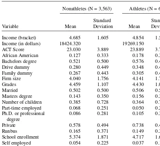
Table 1
Descriptive Statistics for CIRP Data
Nonathletes (N = 3,563) Athletes (N = 646)
Standard Standard
Variable Mean Deviation Mean Deviation
Income (bracket) 4.685 1.605 4.854 1.516
Income (in dollars) 18424.320 19269.150
ACT Score 23.030 3.889 23.889 3.785
African American 0.127 0.333 0.178 0.383
Bachelors degree 0.521 0.500 0.576 0.495
Drive dummy 0.280 0.449 0.348 0.477
Family dummy 0.267 0.443 0.305 0.461
Firm size 4.040 1.756 4.141 1.722
Grades 4.459 1.107 4.430 1.030
Married 0.502 0.500 0.506 0.500
Masters degree 0.143 0.350 0.156 0.363
Number of children 0.385 0.728 0.364 0.708
Part-time employed 0.068 0.251 0.050 0.217
Ph.D. or professional 0.086 0.281 0.105 0.307
degree
Private 0.578 0.494 0.738 0.440
Runbus 0.165 0.371 0.149 0.356
School enrollment 5.374 1.871 4.717 1.650
Self employed 0.054 0.225 0.037 0.189
Veteran 0.029 0.169 0.006 0.079
Well dummy 0.144 0.351 0.161 0.368
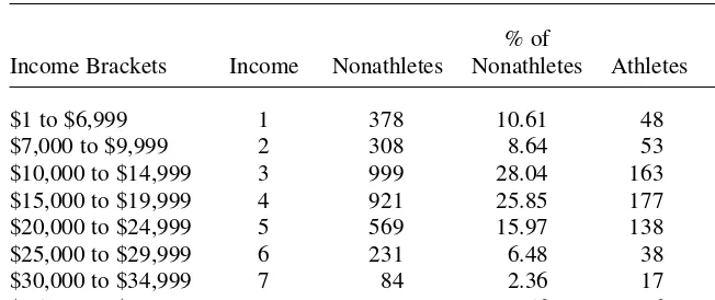
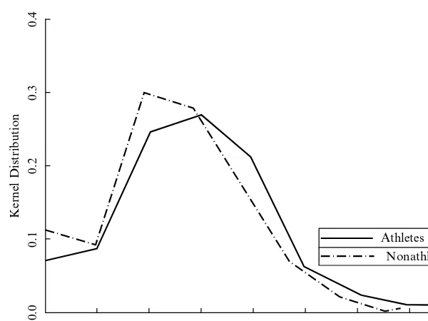
and 9 = $40,000, or more. The distribution of athletes, and nonathletes across income intervals is not identical. Table 2 and Figure 1 show that a slightly higher percentage of athletes are in the higher income brackets, which most likely accounts for the slightly higher average wage enjoyed by athletes.
In addition to income, Table 1 shows that athletes seem to enjoy a slight advantage in certain other categories. A higher percentage of athletes completed their bachelors, masters, and doctoral or professional degrees. Athletes were more likely to attend a private institution and reported themselves to be on average more driven and more likely to have a goal to be financially well-off compared with nonathletes. Neither group had a significant average advantage regarding ACT scores and course grades, but choice of school and motivation seemed to differ between the two groups. They were less likely than nonathletes to want to own their own business. Each of these variables were included as control variables because individuals with a strong com-petitive drive, a goal to be financially well-off, and a motivation to own their own business would be expected to earn higher wages, ceteris paribus. In the statistical analysis to follow, possessing these traits also might make it more likely for an indi-vidual to play competitive athletics, and failure to address these traits could cause a bias in the coefficient of the ATHLETEvariable.
IV. Results
A. Distribution Tests
Before jumping into the regression, we feel it necessary to perform two distributional tests. First, we want to establish that the distribution of wages between athletes, and nonathletes are significantly different from one another. Second, we will test whether the distribution of wages is dependent on athletic participation. Performing these tests Table 2
Income Brackets
% of % of
Income Brackets Income Nonathletes Nonathletes Athletes Athletes
$1 to $6,999 1 378 10.61 48 7.43
$7,000 to $9,999 2 308 8.64 53 8.20
$10,000 to $14,999 3 999 28.04 163 25.23
$15,000 to $19,999 4 921 25.85 177 27.40
$20,000 to $24,999 5 569 15.97 138 21.36
$25,000 to $29,999 6 231 6.48 38 5.88
$30,000 to $34,999 7 84 2.36 17 2.63
$35,000 to $39,999 8 20 0.56 6 0.93
$40,000 or more 9 53 1.49 6 0.93
not only strengthens the argument for inclusion of the ATHLETEvariable on the right-hand side of our wage regression, but it makes the argument that athletic participation has a significant impact on the wages of former college students.
A number of kernel-based tests measure the equality of distributions (for example, see Li 1996); however, generally they require that the underlying variable of interest is continuous in nature. As previously stated, the variable of interest is ordered and categorical, and thus any kernel-based test used requires a kernel function equipped for discrete data. For this reason, we select the Li, Maasoumi, and Racine (2004) non-parametric test for equality of distributions with mixed categorical and continuous data. In our particular case, we are interested in testing whether the probability den-sity function of wages for former college athletes is significantly different from that of nonathletes. Intuitively, if the null hypothesis is rejected, then an investigation of why these two distributions are significantly different may be warranted. With these data, we firmly reject the null hypothesis (p-value = 0.0071).
After establishing a statistical difference between two wage distributions, it is pru-dent to test whether explanatory variables have a deterministic effect on the distribu-tion of wages. The quesdistribu-tion now becomes, does athletic participadistribu-tion influence the distribution of wages? If the ATHLETEvariable is found to significantly affect the sta-bility of the conditional probasta-bility density function, then a strong argument can be made as to why this variable should be included in the wage regression. Here we employ Racine’s (2002) invariance test. This test examines the validity of the null hypothesis, which states that an underlying distribution does not change with partic-ular values of a conditioning variable. To test the null, a gradient is constructed using
1 2 3 4 5 6 7 8 9
0.0
0.1
0.2
0.3
0.4
Kernel Distribution
Athletes Nonathletes
Figure 1
kernel estimates of the conditional probability density function with respect to the conditioning variable of interest, namely the ATHLETEvariable. Intuitively, if we reject the null hypothesis, it is argued that athletic participation has a statistically sig-nificant effect on the distribution of wages. We find that it does by rejecting the null at the 1 percent level of significance (p-value = 0.0005).
B. Regression Results
When encountering a situation in which a regression must be estimated using a lim-ited dependent variable, econometricians often use an ordered logit model.5However,
using this method not only requires several restrictive assumptions, but it also limits discussion to calculating self-determined marginal effects, and makes it difficult to investigate the returns to athletic participation for specific occupations. The nonpara-metric method we use allows for a more straightforward and flexible interpretation of the regression coefficients estimated.
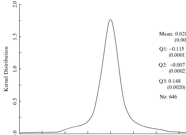
Given the number of parameters obtained from the Generalized Kernel Estimation procedure, it is tricky to present results. Unfortunately no widely accepted presenta-tion format exists. Therefore, in Figure 2, we give the mean, and the 25th, 50th, and 75th percentile along with their respective bootstrapped standard errors (labeled Quartile 1, 2, and 3), as well as a kernel density plot of the coefficients for the athletic participation variable for each athlete included in the data set (by definition, the ath-letic participation coefficient for all nonathletes is zero). Each coefficient represents the impact on earnings (category) for a one unit increase of the associated indepen-dent variable (in other words, ATHLETEgoing from 0 to 1).6
One consideration is important in interpreting the ATHLETEcoefficient. For the coefficient to be unbiased, ATHLETEmust be truly exogenous—implying athletic sta-tus must be randomly assigned. However, it is possible students become athletes because they are innately motivated and disciplined—qualities that are unobservable but positively correlated with earnings (Duncan and Dunifon 1998). If this is the case, athletes may earn more not because universities provide value-added, but because bet-ter students become athletes. There are two ways to get at this potential bias, though each is imperfect. One possibility is to model athletic participation using a selection rule, and then account for this selectivity in the earnings equation (Willis and Rosen 1979). For this approach to work, one ideally should identify factors that affect ath-letic prowess such as height, and weight (unavailable in the data) but that are unre-lated to earnings. The problem finding such variables is at best tricky. Participating in high school athletics is a possibility, but this variable imperfectly predicts collegiate athletic participation, and besides may be correlated with earnings. A second, but also imperfect, approach is to include motivational variables in the original earnings func-tion in order to hold constant the type “drive” that inspires athletes, but also raises earnings. We adopt this latter approach because the data contain two such variables: first, a dummy categorical variable indicating whether the respondent rates himself in
5. When estimating an ordered logit model while using the same setup as LC, a coefficient of 0.269 (stan-dard error of 0.078) for the ATHLETEvariable is obtained.
the highest 10 percent in “drive, and ambition” (Drive Dummy); and second, a dummy categorical variable indicating that being “well-off financially is an important goal” (Well Dummy). Perhaps more importantly, because our true goal is to compare our nonparametric approach to LC, we follow their lead to treat ATHLETEas exoge-nous by assuming innate athletic ability to be a god-given talent.
The mean of the coefficients for the ATHLETEvariable, 0.028, indicates that for-mer college athletes are in a 0.028 higher earnings category than nonathletes, ceteris paribus. Because most income categories represent a $5,000 wage gap, this coefficient can be interpreted as approximately a $140 wage benefit. Although qualitatively sim-ilar, this is smaller than the 4 percent premium reported by LC. But the variation in individual wage premiums is more interesting. Less than half the college athletes actually receive a positive gain. The median of the coefficients (Q2) is negative, implying a skewed distribution with more than half of former college athletes actually earning lower wages than nonathletes, ceteris paribus.
Discussing individual variation in parameter values is one of the major benefits we gain by using the nonparametric technique. Although we found that on average ath-letes obtain a wage premium, we were able to show that over half of them did not. Simply stereotyping all athletes under one estimate is misleading. For example, the typical parametric approach, such as used by LC, suggests that athletes earn higher wages than nonathletes, ceteris paribus. If individuals choosing whether to participate in college athletics take this information as a given, it could affect their decision-making. Given the positive coefficient on ATHLETEfound by LC, individuals may decide to participate in sports because they believe that their wages will rise in the
−2.0 −1.5 −1.0 −0.5 0.0 0.5 1.0 1.5 2.0
0.0
0.5
1.0
1.5
2.0
Kernel Distribution
Mean: 0.028 (0.0019)
Q1: −0.115 (0.0001)
Q2: −0.007 (0.0002)
Q3: 0.148 (0.0020)
Νο: 646
Figure 2
future. Similarly, universities may opt for sports programs believing that individual students necessarily benefit. However, our result shows that the wage premium is not uniform across athletes. Although some athletes enjoy large wage benefits, others earn less than nonathletes. Thus, for students, the more appropriate question is not whether to participate in sports, but the more specific question should be, if an indi-vidual participates in a sport, in which occupations will that indiindi-vidual most likely earn a wage premium over nonathletes?
C. Results by Occupation
Table 3 shows the estimates on the ATHLETEvariable for four job categories; as well as for a fifth category depicting all other occupations combined. The four occupations, high school teaching, business, military, and manual labor are ones with a significant number of former athletes (arbitrarily chosen as those occupations with at least 35 athletes). For the latter three occupations (business, military, and manual labor), the mean, and median are positive, indicating that a wage premium is present for a major-ity of athletes in those occupations. Intuitive arguments could be made that skills obtained, or improved during athletic participation would justify wage premiums in these occupations. Teamwork skills, and an enhanced competitive drive to succeed could be useful in the business world. Physical strength, and other athletic attributes may make manual laborers and military professionals more productive at their jobs, justifying higher wages. The ability to apply strategic thinking, and adjust a particu-lar strategy during a game may be particuparticu-larly important, while using military tactics may be important during a business negotiation, or when operating as a team to per-form some physical task. Many of these reasons apply to the conglomerate occupa-tion, as well.
Although most job categories were associated with wage premiums, the high school teaching occupation was not. In teaching, a majority of former college athletes earn lower wages, ceteris paribus, as compared with nonathletes in this category. Although we will shortly discuss potential explanations of this observation, a wage premium can affect occupational choice. Specifically one would expect former ath-letes to enter jobs where they earn high wages, and shy away from jobs where they do not. But this is not the case for athletes.
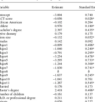
Table 4 reports the results of a logit model where the binary dependent variable, HSTEACHER, takes a value one if an individual reported high school teaching as an occupation, zero otherwise. In this data, former college athletes were found to be more likely to select high school teaching as an occupation despite earning lower wages. Similarly, we found this result to hold on population subsamples such as for African Americans. Several arguments can be levied to explain this behavior, but no evidence in the data clearly supports any claim in particular.
The Journal of Human Resources
Table 3
Wage Premiums for Select Occupations
Occupation Mean Q1 Q2 Q3 Nn Wage (n) Na Wage (a)
High School Teacher −0.0550 −0.0882 −0.0313 −0.0021 190 3.96 66 3.87
0.0006* 0.0007* 0.0002* 0.0002*
Business 0.0643 −0.1658 0.0018 0.0643 1144 5.13 187 5.37
0.0005* 0.0005* 0.0000* 0.0005*
Military 0.0169 −0.0887 0.0478 0.2149 169 4.69 35 5.00
0.0008* 0.0007* 0.0002* 0.0021*
Manual labor 0.0809 −0.0905 0.0265 0.2073 605 4.36 67 4.53
0.0010* 0.0005* 0.0002* 0.0150*
All other occupations 0.0188 −0.1199 0.0001 0.1380 1455 4.59 291 4.80
0.0008* 0.0018* 0.0001 0.0018*
All occupations 0.0280 −0.1150 −0.0070 0.1480 3563 4.69 646 4.85
0.0019* 0.0001* 0.0002* 0.0020*
governmental organization is not allowed by law to discriminate against any particu-lar group. The accessibility and attractiveness of teaching may explain why African American former college athletes are more likely to choose this profession.
Several other theories are worth mentioning. If athletics fosters an increased affec-tion for a school, then an athlete may wish to return to his high school to work. Athletes also may wish to pursue coaching. Because high school teachers often serve as coaches, this desire may be reflected in their occupational choice decision. Even if for-mer athletes choosing this profession realize they will be expected to earn lower aver-age waver-ages, the increased utility generated by coaching may offset any monetary losses. Table 4
Logit Model—Determinants of Becoming a High School Teacher
Variable Estimate Standard Error
Intercept −3.004 0.740
ACT score −0.056 0.026*
African American −0.102 0.264
Athlete 0.970 0.180*
Bachelor’s degree 2.397 0.435*
Drive dummy 0.179 0.175
Firm size −0.132 0.052*
Grades 0.142 0.092
Major1 −0.899 0.466*
Major2 −1.040 0.240*
Major3 −0.791 0.295*
Major4 −3.254 0.478*
Major5 −3.295 0.733*
Major6 −1.244 0.300*
Major7 −1.830 0.741*
Major8 δ δ
Major9 −1.637 0.245*
Major10 −1.041 0.761
Major11 −1.267 0.545*
Married 0.176 0.173
Master’s degree 2.418 0.466*
Number of children −0.161 0.137
Ph.D. or professional degree 0.211 0.743
Private 0.020 0.227
Runbus −0.901 0.306*
School enrollment 0.032 0.058
Veteran −0.047 0.541
Regardless of the reason(s) for becoming teachers, a relatively large supply of for-mer athletes could exert downward wage pressure in the teaching occupation. If a labor market is inordinately supplied with individuals possessing similar traits, then that group’s wages could be lower than comparably skilled workers in other markets. For example, if many former athletes are trying to become physical education teach-ers, then the wages of physical education teachers could be lower than other teachers.
V. Conclusion
Estimating the impact of individual behavior is an important aspect of social research. Often outcomes can be measured in monetary units. When this is the case, one can estimate an earnings function to determine how an individual’s actions affect his or her earnings. In most cases, parametric models are used. However, para-metric models have certain restrictions regarding functional form. In addition, they are usually specified in ways to yield a single coefficient estimate.
One such example is the effect of a student’s participation in college athletics on earn-ings years after leaving college, a topic not well studied because of the paucity of data. However, in one such study Long and Caudill (1991) find that college athletes earn about a 4 percent positive return from collegiate sports. Because of certain data restrictions (a categorical dependent variable) they use Nelson’s (1976) maximum likelihood proce-dure, but as with most parametric procedures, that paper limits itself to obtaining a sin-gle coefficient without exploring how robust their findings are across the population.
This paper reexamines the issue using a new technique. The Li-Racine Generalized Kernel Estimation procedure is able to assess the impact of an exogenous variable within a model containing an ordered categorical dependent variable along with con-tinuous, unordered, and ordered categorical regressors. Of course, the beauty of the technique is its ability to estimate coefficients for each individual so that one can assess the impact of athletic participation across the sample.
This paper examines the CIRP data. Unlike past studies, we find that the wage premiums associated to former college athletes are not uniform. Rather, athletes earn between a 1.5, and 9 percent average wage premium in business, manual labor, and military careers, but nonetheless enter teaching occupations with a higher prob-ability than nonathletes despite facing an average wage deficiency of 8 percent. Whereas wage premiums in the former three occupations conform to the human capital type matching models of occupational choice (Polachek 1981), the latter result regarding teaching are consistent with nonpecuniary incentives explaining occupational choice. This latter result regarding nonpecuniary motivators implies broader implications than usually inferred from typical economics models based solely on pecuniary factors.
Appendix 1 Variable Definitions
Variable Meaning
ACT Score Score on American College Test (range from 9 to 30) African American 1 if African American, 0 otherwise
Athlete 1 if earned a varsity letter in college, 0 otherwise Bachelor’s degree 1 if holds bachelors degree, 0 otherwise
Business 1 if individual reported occupation as business clerical, business management or business sales, 0 otherwise Drive dummy 1 if individual rates themselves in the highest 10 percent
to “drive to achieve,” 0 otherwise
Family dummy 1 if an individual reported that having a family was an important goal, 0 otherwise
Firm size Number of employees in firm individual works for, reported in categories
Grades Self reported average college grades (A to F scale) Manual labor 1 if individual reported occupation as skilled, semi-skilled
or unskilled labor, 0 otherwise
MAJXX Represents various college majors (See Appendix 3) Married 1 if married, 0 otherwise
Masters degree 1 if holds masters degree, 0 otherwise
Military 1 if individual reported occupation as military career, 0 otherwise
Number of children Number of offspring
OCCXX Represents various occupations (see Appendix 2) Part-time employed 1 if an individual was employed part-time, 0 otherwise Ph.D. or professional 1 if holds Ph.D. or advanced professional degree,
degree 0 otherwise
Private 1 if college attended was a privately owned institution, 0 otherwise
Runbus 1 if an individual reported that owning their own business was a goal, 0 otherwise
School enrollment Total enrollment of college, reported in categories Self-employed 1 if individual was self-employed, 0 otherwise Teacher 1 if individual reported occupation as secondary or
elementary teacher, 0 otherwise Veteran 1 if military veteran, 0 otherwise
1 Architecture
12 Other arts & humanities 13 Biology (general)
References
Aitchison, John, and Colin G. G. Aitken. 1976. “Multivariate Binary Discrimination by the Kernel Method.” Biometrika63(3):413–20.
Astin, Alexander. 1982. Minorities in American Higher Education. San Francisco: Jossey-Bass.
Barron, John M., Bradley T. Ewing, and Glen R. Waddell. 2000. “The Effects of High School Athletic Participation on Education and Labor Market Outcomes.” Review of Economics and Statistics82(3):409–21.
Duncan, Greg J., and Rachel Dunifon. 1998. “ ‘Soft-Skills’ and Long-Run Labor Market Success.” Research in Labor Economics17:123–49.
Eide, Eric R., and Nick Ronan. 2001. “Is Participation in High School Athletics an Investment or a Consumption Good? Evidence from High School and Beyond.” Economics of
Education Review20(5):431–42.
Ewing, Bradely T. 1995. “High School Athletics and the Wages of Black Males.” Review of Black Political Economy24(1):65–78.
Falk, William W., Carolyn K. Falkowski, and Thomas A. Lyson. 1981. “Some Plan to Become Teachers: Further Elaboration and Specification.” Sociology of Education54(1): 64–9.
Hall, Peter, Jeff Racine, and Qi Li. 2004. “Cross-Validation and the Estimation of Conditional Probability Densities.” Journal of The American Statistical Association 99(468):1015–26.
Kniesner, Thomas, and Qi Li. 2002. “Nonlinearity in Dynamic Adjustment: Semiparametric Estimation of Panel Labor Supply.” Empirical Economics27(1):131–48.
Li, Qi. 1996. “Nonparametric Testing of Closeness between Two Unknown Distribution Functions.” Econometric Reviews15(3):261–74.
Li, Qi, and Desheng Ouyang. 2005. “Uniform Convergence Rate of Kernel Estimation with Mixed Categorical and Continuous Data.” Economics Letters86(2):291–6.
Li, Qi, Esfandiar Maasoumi, and Jeff Racine. 2004. “A Nonparametric Test for the Equality of Distributions With Mixed Categorical and Continuous Data.” Hamilton: McMaster University. Unpublished.
Li, Qi, and Jeff Racine. 2004. “Cross-Validated Local Linear Nonparametric Regression.” Statistica Sinica14(2):485–512.
––––––. 2006. Nonparametric Econometrics: Theory and Practice. Princeton: Princeton University Press. Forthcoming.
Long, James, and Steven Caudill. 1991. “The Impact of Participation in Intercollegiate Athletics on Income and Graduation.” Review of Economics and Statistics73(3): 525–31.
N ©. Nonparametric software by Jeff Racine (http://www.economics.mcmaster.ca/racine/). NCAA. 2004. “Revenues and Expenses of Intercollegiate Athletics Programs.”
(http://www.ncaa.org).
––––––. 2004. “NCAA Facts.” (http://www.ncaa.org).
Nelson, Forrest. 1976. “On a General Computer Algorithm for the Analysis of Models with Limited Dependent Variables.” Annals of Economic and Social Measurement 5:493–509.
Pagan, Adrian, and Aman Ullah. 1999. Nonparametric Econometrics.Cambridge: Cambridge University Press.
Racine, Jeff. 2002. “A Consistent Nonparametric Distributional Invariance Test.” Hamilton: McMaster University. Unpublished.
Racine, Jeff, and Qi Li. 2004. “Nonparametric Estimation of Regression Functions with both Categorical and Continuous Data.” Journal of Econometrics119(1): 99–130.
Schwarzweller, Harry K., and Thomas A. Lyson. 1978. “Some Plan to Become Teachers: Determinants of Career Specification among Rural Youths in Norway, Germany, and the United States.” Sociology of Education51(1):29–43.
Wang, Min-Chiang, and John van Ryzin. 1981. “A Class of Smooth Estimators for Discrete Estimation.” Biometrika68(1):301–9.