Computer Vision
and Applications
ACADEMIC PRESS ("AP") AND ANYONE ELSE WHO HAS BEEN INVOLVED IN THE CREATION OR PRODUCTION OF THE ACCOMPANYING CODE ("THE PRODUCT") CANNOT AND DO NOT WARRANT THE PERFORMANCE OR RESULTS THAT MAY BE OBTAINED BY USING THE PRODUCT. THE PRODUCT IS SOLD "AS IS" WITHOUT WARRANTY OF MERCHANTABILITY OR FITNESS FOR ANY PARTICULAR PURPOSE. AP WARRANTS ONLY THAT THE MAGNETIC CD-ROM(S) ON WHICH THE CODE IS RECORDED IS FREE FROM DEFECTS IN MATERIAL AND FAULTY WORKMANSHIP UNDER THE NORMAL USE AND SERVICE FOR A PERIOD OF NINETY (90) DAYS FROM THE DATE THE PRODUCT IS DELIVERED. THE PURCHASER’S SOLE AND EXCLUSIVE REMEDY IN THE VENT OF A DEFECT IS EXPRESSLY LIMITED TO EITHER REPLACEMENT OF THE CD-ROM(S) OR REFUND OF THE PURCHASE PRICE,AT AP’S SOLE DISCRETION.
IN NO EVENT,WHETHER AS A RESULT OF BREACH OF CONTRACT,WARRANTY,OR TORT (INCLUDING NEGLIGENCE),WILL AP OR ANYONE WHO HAS BEEN INVOLVED IN THE CRE-ATION OR PRODUCTION OF THE PRODUCT BE LIABLE TO PURCHASER FOR ANY DAM-AGES,INCLUDING ANY LOST PROFITS,LOST SAVINGS OR OTHER INCIDENTAL OR CON-SEQUENTIAL DAMAGES ARISING OUT OF THE USE OR INABILITY TO USE THE PRODUCT OR ANY MODIFICATIONS THEREOF,OR DUE TO THE CONTENTS OF THE CODE,EVEN IF AP HAS BEEN ADVISED ON THE POSSIBILITY OF SUCH DAMAGES,OR FOR ANY CLAIM BY ANY OTHER PARTY.
ANY REQUEST FOR REPLACEMENT OF A DEFECTIVE CD-ROM MUST BE POSTAGE PREPAID AND MUST BE ACCOMPANIED BY THE ORIGINAL DEFECTIVE CD-ROM,YOUR MAILING AD-DRESS AND TELEPHONE NUMBER,AND PROOF OF DATE OF PURCHASE AND PURCHASE PRICE. SEND SUCH REQUESTS,STATING THE NATURE OF THE PROBLEM,TO ACADEMIC PRESS CUSTOMER SERVICE,6277 SEA HARBOR DRIVE,ORLANDO,FL 32887,1-800-321-5068. AP SHALL HAVE NO OBLIGATION TO REFUND THE PURCHASE PRICE OR TO RE-PLACE A CD-ROM BASED ON CLAIMS OF DEFECTS IN THE NATURE OR OPERATION OF THE PRODUCT.
SOME STATES DO NOT ALLOW LIMITATION ON HOW LONG AN IMPLIED WARRANTY LASTS,NOR EXCLUSIONS OR LIMITATIONS OF INCIDENTAL OR CONSEQUENTIAL DAM-AGE,SO THE ABOVE LIMITATIONS AND EXCLUSIONS MAY NOT APPLY TO YOU. THIS WAR-RANTY GIVES YOU SPECIFIC LEGAL RIGHTS,AND YOU MAY ALSO HAVE OTHER RIGHTS WHICH VARY FROM JURISDICTION TO JURISDICTION.
Computer Vision
and Applications
A Guide for Students and Practitioners
Editors
Bernd Jähne
Interdisciplinary Center for Scientific Computing University of Heidelberg,Heidelberg,Germany
and
Scripps Institution of Oceanography University of California,San Diego
Horst Haußecker
Xerox Palo Alto Research Center
Copyright © 2000 by Academic Press.
All rights reserved.
No part of this publication may be reproduced or transmitted in any form or by any means, electronic or mechanical, including photocopy, recording, or any information storage and retrieval system, without permission in writing from the publisher.
Requests for permission to make copies of any part of the work should be mailed to: Permissions Department, Harcourt, Inc., 6277 Sea Harbor Drive, Orlando, Florida, 32887-6777.
ACADEMIC PRESS
A Harcourt Science and Technology Company
525 B Street, Suite 1900, San Diego, CA 92101-4495, USA http://www.academicpress.com
Academic Press
24-28 Oval Road, London NW1 7DX, UK http://www.hbuk.co.uk/ap/
Library of Congress Catalog Number: 99-68829
International Standard Book Number: 0–12–379777-2
Contents
Preface xi
Contributors xv
1 Introduction 1
B. Jähne
1.1 Components of a vision system . . . 1
1.2 Imaging systems . . . 2
1.3 Signal processing for computer vision . . . 3
1.4 Pattern recognition for computer vision . . . 4
1.5 Performance evaluation of algorithms . . . 5
1.6 Classes of tasks. . . 6
1.7 References . . . 8
I Sensors and Imaging 2 Radiation and Illumination 11 H. Haußecker 2.1 Introduction . . . 12
2.2 Fundamentals of electromagnetic radiation. . . 13
2.3 Radiometric quantities . . . 17
2.4 Fundamental concepts of photometry . . . 27
2.5 Interaction of radiation with matter. . . 31
2.6 Illumination techniques. . . 46
2.7 References . . . 51
3 Imaging Optics 53 P. Geißler 3.1 Introduction . . . 54
3.2 Basic concepts of geometric optics . . . 54
3.3 Lenses . . . 56
3.4 Optical properties of glasses . . . 66
3.5 Aberrations . . . 67
3.6 Optical image formation . . . 75
3.7 Wave and Fourier optics . . . 80
3.8 References . . . 84
4 Radiometry of Imaging 85 H. Haußecker
4.1 Introduction . . . 85
4.2 Observing surfaces. . . 86
4.3 Propagating radiance . . . 88
4.4 Radiance of imaging. . . 91
4.5 Detecting radiance . . . 94
4.6 Concluding summary . . . 108
4.7 References . . . 109
5 Solid-State Image Sensing 111 P. Seitz 5.1 Introduction . . . 112
5.2 Fundamentals of solid-state photosensing . . . 113
5.3 Photocurrent processing . . . 120
5.4 Transportation of photosignals. . . 127
5.5 Electronic signal detection . . . 130
5.6 Architectures of image sensors. . . 134
5.7 Color vision and color imaging . . . 139
5.8 Practical limitations of semiconductor photosensors. . . 146
5.9 Conclusions . . . 148
5.10References . . . 149
6 Geometric Calibration of Digital Imaging Systems 153 R. Godding 6.1 Introduction . . . 153
6.2 Calibration terminology . . . 154
6.3 Parameters influencing geometrical performance . . . 155
6.4 Optical systems model of image formation . . . 157
6.5 Camera models . . . 158
6.6 Calibration and orientation techniques. . . 163
6.7 Photogrammetric applications . . . 170
6.8 Summary . . . 173
6.9 References . . . 173
7 Three-Dimensional Imaging Techniques 177 R. Schwarte, G. Häusler, R. W. Malz 7.1 Introduction . . . 178
7.2 Characteristics of 3-D sensors . . . 179
7.3 Triangulation . . . 182
7.4 Time-of-flight (TOF) of modulated light . . . 196
7.5 Optical Interferometry (OF) . . . 199
7.6 Conclusion . . . 205
Contents vii
II Signal Processing and Pattern Recognition
8 Representation of Multidimensional Signals 211
B. Jähne
8.1 Introduction . . . 212
8.2 Continuous signals. . . 212
8.3 Discrete signals . . . 215
8.4 Relation between continuous and discrete signals . . . 224
8.5 Vector spaces and unitary transforms . . . 232
8.6 Continuous Fourier transform (FT) . . . 237
8.7 The discrete Fourier transform (DFT) . . . 246
8.8 Scale of signals . . . 252
8.9 Scale space and diffusion. . . 260
8.10Multigrid representations . . . 267
8.11 References . . . 271
9 Neighborhood Operators 273 B. Jähne 9.1 Basics . . . 274
9.2 Linear shift-invariant filters . . . 278
9.3 Recursive filters. . . 285
9.4 Classes of nonlinear filters. . . 292
9.5 Local averaging . . . 296
9.6 Interpolation. . . 311
9.7 Edge detection . . . 325
9.8 Tensor representation of simple neighborhoods. . . 335
9.9 References . . . 344
10 Motion 347 H. Haußecker and H. Spies 10.1 Introduction . . . 347
10.2 Basics: flow and correspondence. . . 349
10.3 Optical flow-based motion estimation . . . 358
10.4 Quadrature filter techniques . . . 372
10.5 Correlation and matching . . . 379
10.6 Modeling of flow fields . . . 382
10.7 References . . . 392
11 Three-Dimensional Imaging Algorithms 397 P. Geißler, T. Dierig, H. A. Mallot 11.1 Introduction . . . 397
11.2 Stereopsis . . . 398
11.3 Depth-from-focus . . . 414
11.4 References . . . 435
12 Design of Nonlinear Diffusion Filters 439 J. Weickert 12.1 Introduction . . . 439
12.2 Filter design . . . 440
12.3 Parameter selection . . . 448
12.4 Extensions . . . 451
12.6 Summary . . . 454
12.7 References . . . 454
13 Variational Adaptive Smoothing and Segmentation 459 C. Schnörr 13.1 Introduction . . . 459
13.2 Processing of two- and three-dimensional images. . . 463
13.3 Processing of vector-valued images . . . 474
13.4 Processing of image sequences . . . 476
13.5 References . . . 480
14 Morphological Operators 483 P. Soille 14.1 Introduction . . . 483
14.2 Preliminaries. . . 484
14.3 Basic morphological operators . . . 489
14.4 Advanced morphological operators . . . 495
14.5 References . . . 515
15 Probabilistic Modeling in Computer Vision 517 J. Hornegger, D. Paulus, and H. Niemann 15.1 Introduction . . . 517
15.2 Why probabilistic models? . . . 518
15.3 Object recognition as probabilistic modeling . . . 519
15.4 Model densities . . . 524
15.5 Practical issues . . . 536
15.6 Summary, conclusions, and discussion. . . 538
15.7 References . . . 539
16 Fuzzy Image Processing 541 H. Haußecker and H. R. Tizhoosh 16.1 Introduction . . . 541
16.2 Fuzzy image understanding . . . 548
16.3 Fuzzy image processing systems. . . 553
16.4 Theoretical components of fuzzy image processing . . . 556
16.5 Selected application examples . . . 564
16.6 Conclusions . . . 570
16.7 References . . . 571
17 Neural Net Computing for Image Processing 577 A. Meyer-Bäse 17.1 Introduction . . . 577
17.2 Multilayer perceptron (MLP) . . . 579
17.3 Self-organizing neural networks . . . 585
17.4 Radial-basis neural networks (RBNN) . . . 590
17.5 Transformation radial-basis networks (TRBNN) . . . 593
17.6 Hopfield neural networks . . . 596
17.7 Application examples of neural networks . . . 601
17.8 Concluding remarks . . . 604
Contents ix
III Application Gallery
A Application Gallery 609
A1 Object Recognition with Intelligent Cameras . . . 610 T. Wagner, and P. Plankensteiner
A2 3-D Image Metrology of Wing Roots . . . 612 H. Beyer
A3 Quality Control in a Shipyard . . . 614 H.-G. Maas
A4 Topographical Maps of Microstructures . . . 616 Torsten Scheuermann, Georg Wiora and Matthias Graf
A5 Fast 3-D Full Body Scanning for Humans and Other Objects . 618 N. Stein and B. Minge
A6 Reverse Engineering Using Optical Range Sensors. . . 620 S. Karbacher and G. Häusler
A7 3-D Surface Reconstruction from Image Sequences . . . 622 R. Koch, M. Pollefeys and L. Von Gool
A8 Motion Tracking . . . 624 R. Frischholz
A9 Tracking “Fuzzy” Storms in Doppler Radar Images . . . 626 J.L. Barron, R.E. Mercer, D. Cheng, and P. Joe
A103-D Model-Driven Person Detection . . . 628 Ch. Ridder, O. Munkelt and D. Hansel
A11 Knowledge-Based Image Retrieval . . . 630 Th. Hermes and O. Herzog
A12 Monitoring Living Biomass with in situ Microscopy . . . 632 P. Geißler and T. Scholz
A13 Analyzing Size Spectra of Oceanic Air Bubbles. . . 634 P. Geißler and B. Jähne
A14 Thermography to Measure Water Relations of Plant Leaves. . 636 B. Kümmerlen, S. Dauwe, D. Schmundt and U. Schurr
A15 Small-Scale Air-Sea Interaction with Thermography. . . 638 U. Schimpf, H. Haußecker and B. Jähne
A16 Optical Leaf Growth Analysis . . . 640 D. Schmundt and U. Schurr
A17 Analysis of Motility Assay Data. . . 642 D. Uttenweiler and R. H. A. Fink
A18 Fluorescence Imaging of Air-Water Gas Exchange . . . 644 S. Eichkorn, T. Münsterer, U. Lode and B. Jähne
A19 Particle-Tracking Velocimetry. . . 646 D. Engelmann, M. Stöhr, C. Garbe, and F. Hering
A20Analyzing Particle Movements at Soil Interfaces . . . 648 H. Spies, H. Gröning, and H. Haußecker
A21 3-D Velocity Fields from Flow Tomography Data . . . 650 H.-G. Maas
A23 NOXEmissions Retrieved from Satellite Images . . . 654 C. Leue, M. Wenig and U. Platt
A24 Multicolor Classification of Astronomical Objects. . . 656 C. Wolf, K. Meisenheimer, and H.-J. Roeser
A25 Model-Based Fluorescence Imaging . . . 658 D. Uttenweiler and R. H. A. Fink
A26 Analyzing the 3-D Genome Topology . . . 660 H. Bornfleth, P. Edelmann, and C. Cremer
A27 References . . . 662
Preface
What this book is about
This book offers a fresh approach to computer vision. The whole vision process from image formation to measuring, recognition, or reacting is regarded as an integral process. Computer vision is understood as the host of techniques to acquire, process, analyze, and understand complex higher-dimensional data from our environment for scientific and technical exploration.
In this sense this book takes into account the interdisciplinary na-ture of computer vision with its links to virtually all natural sciences and attempts to bridge two important gaps. The first is between mod-ern physical sciences and the many novel techniques to acquire images. The second is between basic research and applications. When a reader with a background in one of the fields related to computer vision feels he has learned something from one of the many other facets of com-puter vision, the book will have fulfilled its purpose.
This book comprises three parts. The first part,Sensors and Imag-ing, covers image formation and acquisition. The second part,Signal Processing and Pattern Recognition, focuses on processing of the spatial and spatiotemporal signals acquired by imaging sensors. The third part consists of anApplication Gallery, which shows in a concise overview a wide range of application examples from both industry and science. This part illustrates how computer vision is integrated into a variety of systems and applications.
Computer Vision and Applicationswas designed as a concise edition of the three-volume handbook:
Handbook of Computer Vision and Applications
edited by B. Jähne, H. Haußecker, and P. Geißler Vol 1: Sensors and Imaging;
Vol 2: Signal Processing and Pattern Recognition; Vol 3: Systems and Applications
Academic Press, 1999
It condenses the content of the handbook into one single volume and contains a selection of shortened versions of the most important contributions of the full edition. Although it cannot detail every single technique, this book still covers the entire spectrum of computer vision ranging from the imaging process to high-end algorithms and applica-tions. Students in particular can benefit from the concise overview of the field of computer vision. It is perfectly suited for sequential reading into the subject and it is complemented by the more detailedHandbook of Computer Vision and Applications. The reader will find references to the full edition of the handbook whenever applicable. In order to simplify notation we refer to supplementary information in the hand-book by the abbreviations [CVA1, ChapterN], [CVA2, ChapterN], and [CVA3, ChapterN] for the Nth chapter in the first, second and third
volume, respectively. Similarly, direct references to individual sections in the handbook are given by [CVA1, SectionN], [CVA2, SectionN], and [CVA3, SectionN] for section numberN.
Prerequisites
It is assumed that the reader is familiar with elementary mathematical concepts commonly used in computer vision and in many other areas of natural sciences and technical disciplines. This includes the basics of set theory, matrix algebra, differential and integral equations, com-plex numbers, Fourier transform, probability, random variables, and graph theory. Wherever possible, mathematical topics are described intuitively. In this respect it is very helpful that complex mathematical relations can often be visualized intuitively by images. For a more for-mal treatment of the corresponding subject including proofs, suitable references are given.
How to use this book
Preface xiii
for all major computing platforms is included on the CDs. The texts are hyperlinked in multiple ways. Thus the reader can collect the informa-tion of interest with ease. Third, the reader can delve more deeply into a subject with the material on the CDs. They contain additional refer-ence material, interactive software components, code examples, image material, and references to sources on the Internet. For more details see the readme file on the CDs.
Acknowledgments
Writing a book on computer vision with this breadth of topics is a major undertaking that can succeed only in a coordinated effort that involves many co-workers. Thus the editors would like to thank first all contrib-utors who were willing to participate in this effort. Their cooperation with the constrained time schedule made it possible that this concise edition of theHandbook of Computer Vision and Applicationscould be published in such a short period following the release of the handbook in May 1999. The editors are deeply grateful for the dedicated and pro-fessional work of the staff at AEON Verlag & Studio who did most of the editorial work. We also express our sincere thanks to Academic Press for the opportunity to write this book and for all professional advice.
Last but not least, we encourage the reader to send us any hints on errors, omissions, typing errors, or any other shortcomings of the book. Actual information about the book can be found at the editors homepagehttp://klimt.iwr.uni-heidelberg.de.
Contributors
Prof. Dr. John L. Barron
Dept. of Computer Science, Middlesex College
The University of Western Ontario, London, Ontario, N6A 5B7, Canada barron@csd.uwo.ca
Horst A. Beyer
Imetric SA, Technopole, CH-2900 Porrentry, Switzerland imetric@dial.eunet.ch,http://www.imetric.com Dr. Harald Bornfleth
Institut für Angewandte Physik, Universität Heidelberg Albert-Überle-Str. 3-5, D-69120Heidelberg, Germany Harald.Bornfleth@iwr.uni-heidelberg.de
http://www.aphys.uni-heidelberg.de/AG_Cremer/ David Cheng
Dept. of Computer Science, Middlesex College
The University of Western Ontario, London, Ontario, N6A 5B7, Canada cheng@csd.uwo.ca
Prof. Dr. Christoph Cremer
Institut für Angewandte Physik, Universität Heidelberg Albert-Überle-Str. 3-5, D-69120Heidelberg, Germany cremer@popeye.aphys2.uni-heidelberg.de
http://www.aphys.uni-heidelberg.de/AG_Cremer/ Tobias Dierig
Forschungsgruppe Bildverarbeitung, IWR, Universität Heidelberg Im Neuenheimer Feld 368, D-69120Heidelberg
Tobias Dierig@iwr.uni-heidelberg.de http://klimt.iwr.uni-heidelberg.de Stefan Dauwe
Botanisches Institut, Universität Heidelberg
Im Neuenheimer Feld 360, D-69120 Heidelberg, Germany Peter U. Edelmann
Institut für Angewandte Physik, Universität Heidelberg Albert-Überle-Str. 3-5, D-69120Heidelberg, Germany edelmann@popeye.aphys2.uni-heidelberg.de
http://www.aphys.uni-heidelberg.de/AG_Cremer/edelmann Sven Eichkorn
Max-Planck-Institut für Kernphysik, Abteilung Atmosphärenphysik
Saupfercheckweg 1, D-69117 Heidelberg, Germany Sven.Eichkorn@mpi-hd.mpg.de
Dirk Engelmann
Forschungsgruppe Bildverarbeitung, IWR, Universität Heidelberg Im Neuenheimer Feld 368, D-69120Heidelberg
Dirk.Engelmann@iwr.uni-heidelberg.de
http://klimt.iwr.uni-heidelberg.de/˜dengel Prof. Dr. Rainer H. A. Fink
II. Physiologisches Institut, Universität Heidelberg Im Neuenheimer Feld 326, D-69120Heidelberg, Germany fink@novsrv1.pio1.uni-heidelberg.de
Dr. Robert Frischholz
DCS AG, Wetterkreuz 19a, D-91058 Erlangen, Germany frz@dcs.de,http://www.bioid.com
Christoph Garbe
Forschungsgruppe Bildverarbeitung, IWR, Universität Heidelberg Im Neuenheimer Feld 368, D-69120Heidelberg
Christoph.Garbe@iwr.uni-heidelberg.de http://klimt.iwr.uni-heidelberg.de Dr. Peter Geißler
ARRI, Abteilung TFE, Türkenstraße 95, D-80799 München pgeiss@hotmail.com
http://klimt.iwr.uni-heidelberg.de Dipl.-Ing. Robert Godding
AICON GmbH, Celler Straße 32, D-38114 Braunschweig, Germany robert.godding@aicon.de,http://www.aicon.de
Matthias Graf
Institut für Kunststoffprüfung und Kunststoffkunde (IKP), Pfaffenwaldring 32, D-70569 Stuttgart, Germany graf@ikp.uni-stuttgart.de,Matthias.Graf@t-online.de http://www.ikp.uni-stuttgart.de
Hermann Gröning
Forschungsgruppe Bildverarbeitung, IWR, Universität Heidelberg Im Neuenheimer Feld 360, D-69120 Heidelberg, Germany Hermann.Groening@iwr.uni-heidelberg.de
http://klimt.iwr.uni-heidelberg.de David Hansel
FORWISS, Bayerisches Forschungszentrum für Wissensbasierte Systeme Forschungsgruppe Kognitive Systeme, Orleansstr. 34, 81667 München http://www.forwiss.de/
Prof. Dr. Gerd Häusler
Chair for Optics, Universität Erlangen-Nürnberg Staudtstraße 7/B2, D-91056 Erlangen, Germany haeusler@physik.uni-erlangen.de
Contributors xvii
Dr. Horst Haußecker
Xerox Palo Alto Research Center (PARC) 3333 Coyote Hill Road, Palo Alto, CA 94304
hhaussec@parc.xerox.com,http://www.parc.xerox.com Dr. Frank Hering
SAP AG, Neurottstraße 16, D-69190Walldorf, Germany frank.hering@sap.com
Dipl.-Inform. Thorsten Hermes
Center for Computing Technology, Image Processing Department University of Bremen, P.O. Box 33 0440, D-28334 Bremen, Germany hermes@tzi.org,http://www.tzi.org/˜hermes
Prof. Dr. Otthein Herzog
Center for Computing Technology, Image Processing Department University of Bremen, P.O. Box 33 0440, D-28334 Bremen, Germany herzog@tzi.org,http://www.tzi.org/˜herzog
Dr. Joachim Hornegger
Lehrstuhl für Mustererkennung (Informatik 5)
Universität Erlangen-Nürnberg, Martensstraße 3, 91058 Erlangen, Germany hornegger@informatik.uni-erlangen.de
http://www5.informatik.uni-erlangen.de Prof. Dr. Bernd Jähne
Forschungsgruppe Bildverarbeitung, IWR, Universität Heidelberg Im Neuenheimer Feld 368, D-69120Heidelberg
Bernd.Jaehne@iwr.uni-heidelberg.de http://klimt.iwr.uni-heidelberg.de Dr. Paul Joe
King City Radar Station, Atmospheric Environmental Services 4905 Dufferin St., Toronto, Ontario M3H 5T4, Canada joep@aestor.dots.doe.ca
Stefan Karbacher
Chair for Optics, Universität Erlangen-Nürnberg Staudtstraße 7/B2, D-91056 Erlangen, Germany
sbk@physik.uni-erlangen.de,http://www.physik.uni-erlangen.de Prof. Dr.-Ing. Reinhard Koch
Institut für Informatik und Praktische Mathematik
Christian-Albrechts-Universität Kiel, Olshausenstr. 40, D 24098 Kiel, Germany rk@is.informatik.uni-kiel.de
Bernd Kümmerlen
Botanisches Institut, Universität Heidelberg
Im Neuenheimer Feld 360, D-69120 Heidelberg, Germany Dr. Carsten Leue
Institut für Umweltphysik, Universität Heidelberg Im Neuenheimer Feld 229, D-69120Heidelberg, Germany Carsten.Leue@iwr.uni-heidelberg.de
Ulrike Lode
Im Neuenheimer Feld 229, D-69120Heidelberg, Germany http://klimt.iwr.uni-heidelberg.de
Prof. Dr.-Ing. Hans-Gerd Maas
Institute for Photogrammetry and Remote Sensing Technical University Dresden, D-01062 Dresden, Germany maas@rcs.urz.tu-dresden.de
Prof. Dr.-Ing. Reinhard Malz
Fachhochschule Esslingen, Fachbereich Informationstechnik Flandernstr. 101, D-73732 Esslingen
reinhard.malz@fht-esslingen.de
Dr. Hanspeter A. Mallot
Max-Planck-Institut für biologische Kybernetik Spemannstr. 38, 72076 Tübingen, Germany Hanspeter.Mallot@tuebingen.mpg.de http://www.kyb.tuebingen.mpg.de/bu/ Prof. Robert E. Mercer
Dept. of Computer Science, Middlesex College
The University of Western Ontario, London, Ontario, N6A 5B7, Canada mercer@csd.uwo.ca
Dr. Anke Meyer-Bäse
Dept. of Electrical Engineering and Computer Science
University of Florida, 454 New Engineering Building 33, Center Drive PO Box 116130, Gainesville, FL 32611-6130, U.S.
anke@alpha.ee.ufl.edu
Bernhard Minge
VITRONIC Dr.-Ing. Stein Bildverarbeitungssysteme GmbH Hasengartenstrasse 14a, D-65189 Wiesbaden, Germany bm@vitronic.de,http://www.vitronic.de
Dr. Olaf Munkelt
FORWISS, Bayerisches Forschungszentrum für Wissensbasierte Systeme Forschungsgruppe Kognitive Systeme, Orleansstr. 34, 81667 München munkelt@forwiss.de,http://www.forwiss.de/˜munkelt
Dr. Thomas Münsterer
VITRONIC Dr.-Ing. Stein Bildverarbeitungssysteme GmbH Hasengartenstr. 14a, D-65189 Wiesbaden, Germany Phone: +49-611-7152-38,tm@vitronic.de
Prof. Dr.-Ing. Heinrich Niemann
Lehrstuhl für Mustererkennung (Informatik 5)
Universität Erlangen-Nürnberg, Martensstraße 3, 91058 Erlangen, Germany niemann@informatik.uni-erlangen.de
http://www5.informatik.uni-erlangen.de Dr. Dietrich Paulus
Lehrstuhl für Mustererkennung (Informatik 5)
Universität Erlangen-Nürnberg, Martensstraße 3, 91058 Erlangen, Germany paulus@informatik.uni-erlangen.de
Contributors xix
Dipl.-Math. Peter Plankensteiner Intego Plankensteiner Wagner Gbr Am Weichselgarten 7, D-91058 Erlangen ppl@intego.de
Prof. Dr. Ulrich Platt
Institut für Umweltphysik, Universität Heidelberg Im Neuenheimer Feld 229, D-69120Heidelberg, Germany pl@uphys1.uphys.uni-heidelberg.de
http://www.iup.uni-heidelberg.de/urmel/atmos.html Dr. Marc Pollefeys
Katholieke Universiteit Leuven, ESAT-PSI/VISICS Kardinaal Mercierlaan 94, B-3001 Heverlee, Belgium Marc.Pollefeys@esat.kuleuven.ac.be
http://www.esat.kuleuven.ac.be/˜pollefey/ Christof Ridder
FORWISS, Bayerisches Forschungszentrum für Wissensbasierte Systeme Forschungsgruppe Kognitive Systeme, Orleansstr. 34, 81667 München ridder@forwiss.de,http://www.forwiss.de/˜ridder
Dr. Torsten Scheuermann Fraunhofer USA, Headquarters
24 Frank Lloyd Wright Drive, Ann Arbor, MI 48106-0335, U.S. tscheuermann@fraunhofer.org,http://www.fraunhofer.org Dr. Uwe Schimpf
Forschungsgruppe Bildverarbeitung, IWR, Universität Heidelberg Im Neuenheimer Feld 360, D-69120 Heidelberg, Germany Uwe.Schimpf@iwr.uni-heidelberg.de
http://klimt.iwr.uni-heidelberg.de Dr. Dominik Schmundt
Forschungsgruppe Bildverarbeitung, IWR, Universität Heidelberg Im Neuenheimer Feld 360, D-69120 Heidelberg, Germany Dominik.Schmundt@iwr.uni-heidelberg.de
http://klimt.iwr.uni-heidelberg.de/˜dschmun/ Prof. Dr. Christoph Schnörr
Dept. of Math. & Computer Science, University of Mannheim D-68131 Mannheim, Germany
schnoerr@ti.uni-mannheim.de,http://www.ti.uni-mannheim.de Dr. Thomas Scholz
SAP AG, Neurottstraße 16, D-69190Walldorf, Germany thomas.scholz@sap.com
Dr. Ulrich Schurr
Botanisches Institut, Universität Heidelberg
Im Neuenheimer Feld 360, D-69120 Heidelberg, Germany uschurr@botanik1.bot.uni-heidelberg.de
Prof. Dr. Rudolf Schwarte
Institut für Nachrichtenverarbeitung (INV)
Universität-GH Siegen, Hölderlinstr. 3, D-57068 Siegen, Germany schwarte@nv.et-inf.uni-siegen.de
http://www.nv.et-inf.uni-siegen.de/inv/inv.html Prof. Dr. Peter Seitz
Centre Suisse d’Electronique et de Microtechnique SA (CSEM) Badenerstrasse 569, CH-8048 Zurich, Switzerland
peter.seitz@csem.ch,http://www.csem.ch/ Prof. Dr. Pierre Soille
Silsoe Research Institute, Wrest Park
Silsoe, Bedfordshire, MK45 4HS, United Kingdom Pierre.Soille@bbsrc.ac.uk,http://www.bbsrc.ac.uk/ Hagen Spies
Forschungsgruppe Bildverarbeitung, IWR, Universität Heidelberg Im Neuenheimer Feld 368, D-69120Heidelberg
Hagen.Spies@iwr.uni-heidelberg.de http://klimt.iwr.uni-heidelberg.de Dr.-Ing. Norbert Stein
VITRONIC Dr.-Ing. Stein Bildverarbeitungssysteme GmbH Hasengartenstrasse 14a, D-65189 Wiesbaden, Germany st@vitronic.de,http://www.vitronic.de
Michael Stöhr
Forschungsgruppe Bildverarbeitung, IWR, Universität Heidelberg Im Neuenheimer Feld 368, D-69120Heidelberg
Michael.Stoehr@iwr.uni-heidelberg.de http://klimt.iwr.uni-heidelberg.de Hamid R. Tizhoosh
Universität Magdeburg (IPE)
P.O. Box 4120, D-39016 Magdeburg, Germany tizhoosh@ipe.et.uni-magdeburg.de
http://pmt05.et.uni-magdeburg.de/˜hamid/ Dr. Dietmar Uttenweiler
II. Physiologisches Institut, Universität Heidelberg Im Neuenheimer Feld 326, D-69120Heidelberg, Germany dietmar.uttenweiler@urz.uni-heidelberg.de
Prof. Dr. Luc Van Gool
Katholieke Universiteit Leuven, ESAT-PSI/VISICS Kardinaal Mercierlaan 94, B-3001 Heverlee, Belgium luc.vangool@esat.kuleuven.ac.be
http://www.esat.kuleuven.ac.be/psi/visics.html Dr. Thomas Wagner
Contributors xxi
Dr. Joachim Weickert
Dept. of Math. & Computer Science, University of Mannheim D-68131 Mannheim, Germany
Joachim.Weickert@ti.uni-mannheim.de http://www.ti.uni-mannheim.de Mark O. Wenig
Institut für Umweltphysik, Universität Heidelberg Im Neuenheimer Feld 229, D-69120Heidelberg, Germany Mark.Wenig@iwr.uni-heidelberg.de
http://klimt.iwr.uni-heidelberg.de/˜mwenig Georg Wiora
DaimlerChrysler AG, Research and Development Wilhelm-Runge-Str. 11, D-89081 Ulm, Germany georg.wiora@DaimlerChrysler.com
Dr. Christian Wolf
Max-Planck Institut für Astronomie Königstuhl 17, D-69117 Heidelberg cwolf@mpia-hd.mpg.de
1
Introduction
Bernd Jähne
Interdisziplinäres Zentrum für Wissenschaftliches Rechnen (IWR) Universität Heidelberg,Germany
1.1 Components of a vision system . . . 1 1.2 Imaging systems . . . 2 1.3 Signal processing for computer vision . . . 3 1.4 Pattern recognition for computer vision . . . 4 1.5 Performance evaluation of algorithms . . . 5 1.6 Classes of tasks. . . 6 1.7 References . . . 8
1.1
Components of a vision system
Computer vision is a complex subject. As such it is helpful to divide it into its various components or function modules. On this level, it is also much easier to compare a technical system with a biological system. In this sense, the basic common functionality of biological and machine vision includes the following components (see also Table1.1): Radiation source. If no radiation is emitted from the scene or the ob-ject of interest, nothing can be observed or processed. Thus appro-priate illumination is necessary for objects that are themselves not radiant.
Camera. The “camera” collects the radiation received from the object in such a way that the radiation’s origins can be pinpointed. In the simplest case this is just an optical lens. But it could also be a completely different system, for example, an imaging optical spec-trometer, an x-ray tomograph, or a microwave dish.
Sensor. The sensor converts the received radiative flux density into a suitable signal for further processing. For an imaging system nor-mally a 2-D array of sensors is required to capture the spatial dis-tribution of the radiation. With an appropriate scanning system in some cases a single sensor or a row of sensors could be sufficient.
1
Table 1.1: Function modules of human and machine vision Task Human vision Machine vision
Visualization Passive,mainly by re-flection of light from opaque surfaces
Passive and active (controlled il-lumination) using electromagnetic,
Muscle-controlled pupil Motorized apertures,filter wheels, tunable filters
Focusing Muscle-controlled change of focal length
Autofocus systems based on vari-ous principles of distance measure-ments
Irradiance resolution
Logarithmic sensitivity Linear sensitivity,quantization be-tween 8- and 16-bits; logarithmic sensitivity
Tracking Highly mobile eyeball Scanner and robot-mounted cam-eras parallel processing not in general use
Processing unit. It processes the incoming, generally higher-dimen-sional data, extracting suitable features that can be used to measure object properties and categorize them into classes. Another impor-tant component is a memory system to collect and store knowl-edge about the scene, including mechanisms to delete unimportant things.
Actors. Actors react to the result of the visual observation. They be-come an integral part of the vision system when the vision system is actively responding to the observation by, for example,tracking
an object of interest or by using a vision-guided navigation (active vision,perception action cycle).
1.2
Imaging systems
1.3 Signal processing for computer vision 3
Figure 1.1:Chain of steps linking an object property to the signal measured by an imaging system.
It is important to note that the type of answer we receive from these two implicit questions depends on the purpose of the vision system. The answer could be of either a qualitative or a quantitative nature. For some applications it could be sufficient to obtain a qualitative an-swer like “there is a car on the left coming towards you.” The “what” and “where” questions can thus cover the entire range from “there is something,” a specification of the object in the form of a class, to a de-tailed quantitative description of various properties of the objects of interest.
The relation that links the object property to the signal measured by an imaging system is a complex chain of processes (Fig.1.1). Interaction of the radiation with the object (possibly using an appropriate illumi-nation system) causes the object to emit radiation. A portion (usually only a very small part) of the emitted radiative energy is collected by the optical system and perceived as anirradiance(radiative energy/area). A sensor (or rather an array of sensors) converts the received radiation into an electrical signal that is subsequently sampled and digitized to form a digital image as an array of digital numbers.
Onlydirect imaging systems provide a direct point-to-point corre-spondence between points of the objects in the 3-D world and at the image plane.Indirect imagingsystems also give a spatially distributed irradiance but with no such one-to-one relation. Generation of an im-age requires reconstruction of the object from the perceived irradiance. Examples of such imaging techniques include radar imaging, various techniques for spectral imaging, acoustic imaging, tomographic imag-ing, and magnetic resonance imaging.
1.3
Signal processing for computer vision
deal with image processing. Likewise the transforms and applications handbook by Poularikas [4] is not restricted to 1-D transforms.
There are, however, only a few monographs that treat signal pro-cessing specifically for computer vision and image propro-cessing. The monograph by Lim [5] deals with 2-D signal and image processing and tries to transfer the classical techniques for the analysis of time series to 2-D spatial data. Granlund and Knutsson [6] were the first to publish a monograph on signal processing for computer vision and elaborate on a number of novel ideas such as tensorial image processing and nor-malized convolution that did not have their origin in classical signal processing.
Time series are 1-D, signals in computer vision are of higher di-mension. They are not restricted to digital images, that is, 2-D spatial signals (Chapter8). Volumetric sampling,image sequences, and hyper-spectral imagingall result in 3-D signals, a combination of any of these techniques in even higher-dimensional signals.
How much more complex does signal processing become with in-creasing dimension? First, there is the explosion in the number of data points. Already a medium resolution volumetric image with 5123
vox-els requires 128 MB if one voxel carries just one byte. Storage of even higher-dimensional data at comparable resolution is thus beyond the capabilities of today’s computers.
Higher dimensional signals pose another problem. While we do not have difficulty in grasping 2-D data, it is already significantly more de-manding to visualize 3-D data because the human visual system is built only to see surfaces in 3-D but not volumetric 3-D data. The more di-mensions are processed, the more important it is thatcomputer graph-icsandcomputer visionmove closer together.
The elementary framework for lowlevel signal processing for com-puter vision is worked out in Chapters8and9. Of central importance are neighborhood operations (Chapter9), including fast algorithms for local averaging (Section9.5), and accurate interpolation (Section9.6).
1.4
Pattern recognition for computer vision
1.5 Performance evaluation of algorithms 5
includingstereo (Section 11.2), shape from shading and photometric stereo, and depth from focus (Section11.3).
There is little doubt thatnonlinear techniques are crucial for fea-ture extraction in computer vision. However, compared to linear filter techniques, these techniques are still in their infancy. There is also no single nonlinear technique but there are a host of such techniques often specifically adapted to a certain purpose [7]. In this volume, we give an overview of the various classes of nonlinear filter techniques (Section9.4) and focus on a first-order tensor representation of of non-linear filters by combination of non-linear convolution and nonnon-linear point operations (Chapter9.8) and nonlinear diffusion filtering (Chapter12). In principle, pattern classification is nothing complex. Take some appropriate features and partition the feature space into classes. Why is it then so difficult for a computer vision system to recognize objects? The basic trouble is related to the fact that the dimensionality of the in-put space is so large. In principle, it would be possible to use the image itself as the input for a classification task, but no real-world classifi-cation technique—be it statistical, neuronal, or fuzzy—would be able to handle such high-dimensional feature spaces. Therefore, the need arises to extract features and to use them for classification.
Unfortunately, techniques for feature selection have very often been neglected in computer vision. They have not been developed to the same degree of sophistication as classification, where it is meanwhile well understood that the different techniques, especially statistical and neural techniques, can been considered under a unified view [8].
This book focuses in part on some more advanced feature-extraction techniques. An important role in this aspect is played by morphological operators (Chapter14) because they manipulate the shape of objects in images. Fuzzy image processing (Chapter16) contributes a tool to handle vague data and information.
Object recognition can be performed only if it is possible to repre-sent the knowledge in an appropriate way. In simple cases the knowl-edge can just rest in simple models. Probabilistic modeling in com-puter vision is discussed in Chapter15. In more complex cases this is not sufficient.
1.5
Performance evaluation of algorithms
What is the cause of this situation? On the one side, it is certainly true that some problems in computer vision are very hard and that it is even harder to perform a sophisticated error analysis. On the other hand, the computer vision community has ignored the fact to a large extent that any algorithm is only as good as its objective and solid evaluation and verification.
Fortunately, this misconception has been recognized in the mean-time and there are serious efforts underway to establish generally ac-cepted rules for theperformance analysis of computer vision algorithms
[9]. The three major criteria for the performance of computer vision al-gorithms are:
Successful solution of task. Any practitioner gives this a top priority. But also the designer of an algorithm should define precisely for which task it is suitable and what the limits are.
Accuracy. This includes an analysis of the statistical and systematic errors under carefully defined conditions (such as given signal-to-noise ratio(SNR), etc.).
Speed. Again this is an important criterion for the applicability of an algorithm.
There are different ways to evaluate algorithms according to the fore-mentioned criteria. Ideally this should include three classes of studies:
Analytical studies. This is the mathematically most rigorous way to verify algorithms, check error propagation, and predict catastrophic failures.
Performance tests with computer generated images. These tests are useful as they can be carried out under carefully controlled condi-tions.
Performance tests with real-world images. This is the final test for practical applications.
Much of the material presented in this volume is written in the spirit of a careful and mathematically well-founded analysis of the methods that are described although the performance evaluation techniques are certainly more advanced in some areas than in others.
1.6
Classes of tasks
1.6 Classes of tasks 7
Table 1.2:Classification of tasks for computer vision systems
Task References
2-D & 3-D geometry,6
Position,distance A26
Size,area A12
Depth,3-D optical metrology 11.2,A2,A4,A5,A6,A26 2-D form & 2-D shape 14,A13
3-D object shape 6,7,A2,A4,A5,A6,A7
Radiometry-related,2
Reflectivity 2.5
Color A2
Temperature A15,A14
Fluorescence A17,A18,A25,A26 Hyperspectral imaging A22,A23,A24,A26
Motion,10
2-D motion field 10,A16,A17,A19,A20 3-D motion field A19,A21
Spatial structure and texture
Edges & lines 9.7
Local wave number; scale 8.9,10.4,12,13 Local orientation 9.8,13
Texture 9.8
High-level tasks
Segmentation 13,14,A12,A13 Object identification A1,A12
Object classification A1,A22,?? Model- and knowledge-based
recognition and retrieval A1,A11,A12
3-D modeling
3-D object recognition A6,A10,A7 3-D object synthesis A7
An attempt at such a classification is made in Table1.2. The table categorizes both the tasks with respect to 2-D imaging and the analysis of dynamical 3-D scenes. The second column contains references to chapters dealing with the corresponding task.
1.7
References
[1] Oppenheim, A. V. and Schafer, R. W., (1989).Discrete-Time Signal Process-ing. Prentice-Hall Signal Processing Series. Englewood Cliffs, NJ: Prentice-Hall.
[2] Proakis, J. G. and Manolakis, D. G., (1992). Digital Signal Processing. Prin-ciples, Algorithms, and Applications. New York: McMillan.
[3] Madisetti, V. K. and Williams, D. B. (eds.), (1997). The Digital Signal Pro-cessing Handbook. Boca Raton, FL: CRC Press.
[4] Poularikas, A. D. (ed.), (1996).The Transforms and Applications Handbook. Boca Raton, FL: CRC Press.
[5] Lim, J. S., (1990).Two-dimensional Signal and Image Processing. Englewood Cliffs, NJ: Prentice-Hall.
[6] Granlund, G. H. and Knutsson, H., (1995). Signal Processing for Computer Vision. Norwell, MA: Kluwer Academic Publishers.
[7] Pitas, I. and Venetsanopoulos, A. N., (1990).Nonlinear Digital Filters. Prin-ciples and Applications. Norwell, MA: Kluwer Academic Publishers. [8] Schürmann, J., (1996). Pattern Classification, a Unified Viewof Statistical
and Neural Approaches. New York: John Wiley & Sons.
Part I
2
Radiation and Illumination
Horst Haußecker
Xerox Palo Alto Research Center (PARC)
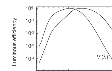
2.1 Introduction . . . 12 2.2 Fundamentals of electromagnetic radiation. . . 13 2.2.1 Electromagnetic waves . . . 13 2.2.2 Dispersion and attenuation . . . 15 2.2.3 Polarization of radiation . . . 15 2.2.4 Coherence of radiation . . . 16 2.3 Radiometric quantities . . . 17 2.3.1 Solid angle . . . 17 2.3.2 Conventions and overview. . . 18 2.3.3 Definition of radiometric quantities. . . 20 2.3.4 Relationship of radiometric quantities . . . 23 2.3.5 Spectral distribution of radiation . . . 26 2.4 Fundamental concepts of photometry . . . 27 2.4.1 Spectral response of the human eye . . . 27 2.4.2 Definition of photometric quantities . . . 28 2.4.3 Luminous efficacy . . . 30 2.5 Interaction of radiation with matter. . . 31 2.5.1 Basic definitions and terminology . . . 32 2.5.2 Properties related to interfaces and surfaces. . . 36 2.5.3 Bulk-related properties of objects . . . 40 2.6 Illumination techniques. . . 46 2.6.1 Directional illumination . . . 47 2.6.2 Diffuse illumination . . . 48 2.6.3 Rear illumination. . . 49 2.6.4 Light and dark field illumination. . . 49 2.6.5 Telecentric illumination . . . 49 2.6.6 Pulsed and modulated illumination. . . 50 2.7 References . . . 51
11
2.1
Introduction
Visual perception of scenes depends on appropriate illumination to vi-sualize objects. The human visual system is limited to a very narrow portion of the spectrum of electromagnetic radiation, calledlight. In some cases natural sources, such as solar radiation, moonlight, light-ning flashes, or bioluminescence, provide sufficient ambient light to navigate our environment. Because humankind was mainly restricted to daylight, one of the first attempts was to invent an artificial light source—fire (not only as a food preparation method).
Computer vision is not dependent upon visual radiation, fire, or glowing objects to illuminate scenes. As soon as imaging detector sys-tems became available other types of radiation were used to probe scenes and objects of interest. Recent developments in imaging sen-sors cover almost the whole electromagnetic spectrum from x-rays to radiowaves (Chapter5). In standard computer vision applications illu-mination is frequently taken as given and optimized to illuminate ob-jects evenly with high contrast. Such setups are appropriate for object identification and geometric measurements. Radiation, however, can also be used to visualize quantitatively physical properties of objects by analyzing their interaction with radiation (Section2.5).
Physical quantities such as penetration depth or surface reflectivity are essential to probe the internal structures of objects, scene geome-try, and surface-related properties. The properties of physical objects therefore can be encoded not only in the geometrical distribution of emitted radiation but also in the portion of radiation that is emitted, scattered, absorbed or reflected, and finally reaches the imaging sys-tem. Most of these processes are sensitive to certain wavelengths and additional information might be hidden in the spectral distribution of radiation. Using different types of radiation allows taking images from different depths or different object properties. As an example, infrared radiation of between 3 and 5µm is absorbed by human skin to a depth of < 1 mm, while x-rays penetrate an entire body without major attenu-ation. Therefore, totally different properties of the human body (such as skin temperature as well as skeletal structures) can be revealed for medical diagnosis.
2.2 Fundamentals of electromagnetic radiation 13
2.2
Fundamentals of electromagnetic radiation
2.2.1 Electromagnetic waves
Electromagnetic radiationconsists of electromagnetic waves carrying energy and propagating through space. Electrical and magnetic fields are alternating with a temporalfrequencyνand a spatialwavelengthλ. The metric units ofνandλare cycles per second (s−1), and meter (m),
respectively. The unit 1 s−1 is also called one hertz (1 Hz). Wavelength
and frequency of waves are related by thespeed of lightc:
c=νλ (2.1)
The speed of light depends on the medium through which the electro-magnetic wave is propagating. In vacuum, the speed of light has the value 2.9979 × 10⁸m s−1, which is one of the fundamental physical
constants and constitutes the maximum possible speed of any object. The speed of light decreases as it penetrates matter, with slowdown being dependent upon the electromagnetic properties of the medium (see Section2.5.2).
Photon energy. In addition to electromagnetic theory, radiation can
be treated as a flow of particles, discrete packets of energy called pho-tons. One photon travels at the speed of lightcand carries the energy
ep=hν=hcλ (2.2)
whereh=6.626×10⁻³⁴J s is Planck’s constant. Therefore the energy
content of radiation is quantized and can only be a multiple ofhνfor a certain frequencyν. While the energy per photon is given by Eq. (2.2), the total energy of radiation is given by the number of photons. It was this quantization of radiation that gave birth to the theory of quantum mechanics at the beginning of the twentieth century.
The energy of a single photon is usually given inelectron volts(1 eV = 1.602×10⁻¹⁹). One eV constitutes the energy of an electron being
accelerated in an electrical field with a potential difference of one volt. Although photons do not carry electrical charge this unit is useful in radiometry, as electromagnetic radiation is usually detected by inter-action of radiation with electrical charges in sensors (Chapter5). In solid-state sensors, for example, the energy of absorbed photons is used to lift electrons from the valence band into the conduction band of a semiconductor. The bandgap energyEgdefines the minimum
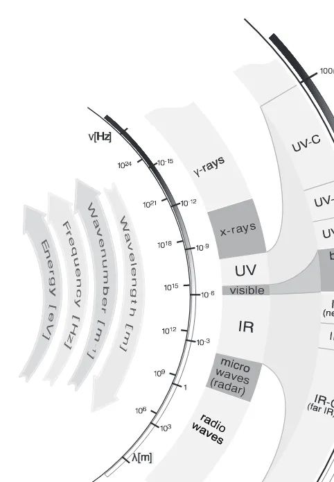
IR-B
Figure 2.1: Spectrum of electromagnetic radiation. (By Sven Mann, University of Heidelberg.)
derived from Eq. (2.2)). Silicon(Si) has a bandgap of 1.1 eV and requires wavelengths below 1.1µm to be detected. This shows why InSb can be used as detector material for infrared cameras in the 3-5µm wave-length region, while silicon sensors are used for visible radiation. It also shows, however, that the sensitivity of standard silicon sensors extends beyond the visible range up to approximately 1µm, which is often neglected in applications (Chapter5).
Electromagnetic spectrum. Monochromatic radiation consists of only
to-2.2 Fundamentals of electromagnetic radiation 15
gether with the standardized terminology1 separating different parts.
Electromagnetic radiation covers the whole range from very high energy cosmic rays with wavelengths in the order of 10−16m (ν = 1024Hz) to
sound frequencies above wavelengths of 106m (ν = 102Hz). Only a
very narrow band of radiation between 380and 780nm is visible to the human eye.
Each portion of the electromagnetic spectrum obeys the same prin-cipal physical laws. Radiation of different wavelengths, however, ap-pears to have different properties in terms of interaction with matter and detectability that can be used for wavelength selective detectors. For the last one hundred years detectors have been developed for ra-diation of almost any region of the electromagnetic spectrum. Recent developments in detector technology incorporate point sensors into in-tegrated detector arrays, which allows setting up imaging radiometers instead of point measuring devices. Quantitative measurements of the spatial distribution of radiometric properties are now available for re-mote sensing at almost any wavelength.
2.2.2 Dispersion and attenuation
A mixture of radiation consisting of different wavelengths is subject to different speeds of light within the medium it is propagating. This fact is the basic reason for optical phenomena such asrefractionand disper-sion. While refraction changes the propagation direction of a beam of radiation passing the interface between two media with different opti-cal properties, dispersion separates radiation of different wavelengths (Section2.5.2).
2.2.3 Polarization of radiation
In electromagnetic theory, radiation is described as oscillating electric and magnetic fields, denoted by the electric field strengthE and the magnetic field strengthB, respectively. Both vector fields are given by the solution of a set of differential equations, referred to asMaxwell’s equations.
In free space, that is, without electric sources and currents, a special solution is aharmonic planar wave, propagating linearly in space and time. As Maxwell’s equations are linear equations, the superposition of two solutions also yields a solution. This fact is commonly referred to as thesuperposition principle. The superposition principle allows us to explain the phenomenon ofpolarization, another important property of electromagnetic radiation. In general, the 3-D orientation of vec-torE changes over time and mixtures of electromagnetic waves show
1International Commission on Illumination (Commission Internationale de
a
E
direction propagation
b
Figure 2.2: Illustration ofalinear andbcircular polarization of electromag-netic radiation. (By C. Garbe, University of Heidelberg.)
randomly distributed orientation directions ofE. If, however, the elec-tromagnetic field vectorEis confined to a plane, the radiation is called
linearly polarized(Fig.2.2a).
If two linearly polarized electromagnetic waves are traveling in the same direction, the resulting electric field vector is given byE=E1+E2.
Depending on the phase shiftΦin the oscillations ofE1andE2, the net
electric field vector E remains linearly polarized (Φ = 0), or rotates around the propagation direction of the wave. For a phase shift of
Φ=90◦, the wave is calledcircularly polarized (Fig.2.2b). The general case consists ofelliptical polarization, that is, mixtures between both cases.
Due to polarization, radiation exhibits different properties in differ-ent directions, such as, for example, directional reflectivity or polariza-tion dependent transmissivity.
2.2.4 Coherence of radiation
Mixtures of electromagnetic waves, which are emitted from conven-tional light sources, do not show any spatial and temporal relation. The phase shifts between the electric field vectorsEand the corresponding orientations are randomly distributed. Such radiation is called incoher-ent.
2.3 Radiometric quantities 17
r φ
s
Figure 2.3:Definition of plane angle.
2.3
Radiometric quantities
2.3.1 Solid angle
In order to quantify the geometric spreading of radiation leaving a source, it is useful to recall the definition of solid angle. It extends the concept of plane angle into 3-D space. Aplane angle θis defined as the ratio of the arc lengths on a circle to the radiusr centered at the point of definition:
θ= s
r (2.3)
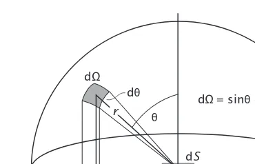
The arc lengths can be considered as projection of an arbitrary line in the plane onto the circle (Fig.2.3). Plane angles are measured in rad (radians). A plane angleθquantifies the angular subtense of a line segment in the plane viewed from the point of definition. A circle has a circumference of 2πr and, therefore, subtends a plane angle of 2πrad. Asolid angleΩis similarly defined as the ratio of an areaAon the surface of a sphere to the square radius, as shown in Fig.2.4:
Ω= A
r2 (2.4)
The area segmentAcan be considered as the projection of an arbitrarily shaped area in 3-D space onto the surface of a sphere. Solid angles are measured in sr (steradian). They quantify the areal subtense of a 2-D surface area in 3-D space viewed from the point of definition. A sphere subtends a surface area of 4πr2, which corresponds to a solid angle of
4πsr. Given a surface areaAthat is tilted under some angleθbetween the surface normal and the line of sight the solid angle is reduced by a factor of cosθ:
Ω= A
r W
x y
z
A
Figure 2.4: Definition of solid angle. (By C. Garbe, University of Heidelberg.)
Table 2.1: Definitions of radiometric quantities (corresponding photometric quantities are defined in Table2.2)
Quantity Symbol Units Definition
Radiant energy Q Ws Total energy emitted by a source or received by a detector
Radiant flux Φ W Total power emitted by a source or received by a detector
Radiant exitance M W m−2 Power emitted per unit surface
area
Irradiance E W m−2 Power received at unit surface
element
Radiant intensity I W sr−1 Power leaving a point on a
sur-face into unit solid angle
Radiance L W m−2sr−1 Power leaving unit projected
sur-face area into unit solid angle
From the definition of angles as ratios of lengths or areas it follows that they have no physical unit. However, it is advisable always to use the artificial units rad and sr when referring to quantities related to angles to avoid confusion. Radiometric and photometric quantities also have to be defined carefully as their meaning cannot be inferred from physical units (Tables2.1and2.2).
2.3.2 Conventions and overview
op-2.3 Radiometric quantities 19
Table 2.2: Definitions of photometric quantities (corresponding radiometric quantities are defined in Table2.1)
Quantity Symbol Units Definition
Luminous energy Qν lm s
Total luminous energy emitted by a source or received by a detector
Luminous flux Φν lm (lumen)
Total luminous power emitted by a source or received by a detector
Luminous exitance Mν lm m−2 Luminous power emittedper unit surface area
Illuminance Eν lm m
−2
= lx (lux)
Luminous power received at unit surface element
Luminous intensity Iν lumen sr
−1
= cd (candela)
Luminous power leaving a point on a surface into unit solid angle
Luminance Lν lumen m
−2sr−1
= cd m−2
Luminous power leaving unit projected surface area into unit solid angle
tics. However, it is not very difficult if some care is taken with regard to definitions of quantities related to angles and areas.
Despite confusion in the literature, there seems to be a trend to-wards standardization of units. (In pursuit of standardization we will use only SI units, in agreement with the International Commission on Illumination CIE. The CIE is the international authority defining termi-nology, standards, and basic concepts in radiometry and photometry. The radiometric and photometric terms and definitions are in com-pliance with the American National Standards Institute (ANSI) report RP-16, published in 1986. Further information on standards can be found at the web sites of CIE (http://www.cie.co.at/cie/) and ANSI (http://www.ansi.org), respectively.)
In this section, the fundamental quantities of radiometry will be defined. The transition to photometric quantities will be introduced by a generic Equation (2.27), which can be used to convert each of these radiometric quantities to its corresponding photometric counterpart.
2.3.3 Definition of radiometric quantities
Radiant energy and radiant flux. Radiation carries energy that can be
absorbed in matter heating up the absorber or interacting with electrical charges.Radiant energyQis measured in units of Joule (1 J = 1 Ws). It quantifies the total energy emitted by a source or received by a detector.
Radiant flux Φis defined as radiant energy per unit time interval
Φ= dQ
dt (2.6)
passing through or emitted from a surface. Radiant flux has the unit watts (W) and is also frequently called radiant power, which corre-sponds to its physical unit. Quantities describing the spatial and ge-ometric distributions of radiative flux are introduced in the following sections.
The units for radiative energy, radiative flux, and all derived quan-tities listed in Table2.1 are based on Joule as the fundamental unit. Instead of theseenergy-derivedquantities an analogous set of photon-derived quantities can be defined based on the number of photons. Photon-derived quantities are denoted by the subscript p, while the energy-based quantities are written with a subscripteif necessary to distinguish between them. Without a subscript, all radiometric quanti-ties are considered energy-derived. Given the radiant energy the num-ber of photons can be computed from Eq. (2.2)
Np= Qee p =
λ
hcQe (2.7)
With photon-based quantities the number of photons replaces the ra-diative energy. The set of photon-related quantities is useful if radia-tion is measured by detectors that correspond linearly to the number of absorbed photons (photon detectors) rather than to thermal energy stored in the detector material (thermal detector).
Photon fluxΦp is defined as the number of photons per unit time
interval
Φp= dNp
dt = λ hc
dQe
dt = λ
hcΦe (2.8)
Similarly, all other photon-related quantities can be computed from the corresponding energy-based quantities by dividing them by the energy of a single photon.
2.3 Radiometric quantities 21
a
dS
b
dS
Figure 2.5:Illustration of the radiometric quantities:aradiant exitance; andb irradiance. (By C. Garbe, University of Heidelberg.)
Radiant exitance and irradiance. Radiant exitanceM defines the
ra-diative fluxemittedper unit surface area M= dΦ
dS (2.9)
of a specified surface. The flux leaving the surface is radiated into the whole hemisphere enclosing the surface elementdSand has to be inte-grated over all angles to obtainM (Fig.2.5a). The flux is, however, not radiated uniformly in angle. Radiant exitance is a function of position on the emitting surface,M=M(x). Specification of the position on the surface can be omitted if the emitted fluxΦis equally distributed over
an extended areaS. In this caseM=Φ/S.
IrradianceEsimilarly defines the radiative fluxincidenton a certain point of a surface per unit surface element
E= ddSΦ (2.10)
Again, incident radiation is integrated over all angles of the enclosing hemisphere (Fig.2.5b). Radiant exitance characterizes an actively radi-ating source while irradiance characterizes a passive receiver surface. Both are measured in W m−2and cannot be distinguished by their units
if not further specified.
Radiant intensity. Radiant intensityIdescribes the angular
distribu-tion of radiadistribu-tion emerging from a point in space. It is defined as radiant flux per unit solid angle
I= dΦ
dΩ (2.11)
and measured in units of W sr−1. Radiant intensity is a function of the
a
Z
Y
X
W q
f
d
b
Z
Y
X
W q
f
d
dS
dS = dS cos q
Figure 2.6: Illustration of radiometric quantities: aradiant intensity; and b radiance. (By C. Garbe, University of Heidelberg.)
θandφ(Fig.2.6). Intensity is usually used to specify radiation emitted frompoint sources, such as stars or sources that are much smaller than their distance from the detector, that is,dxdy≪r2. In order to use it
for extended sources those sources have to be made up of an infinite number of infinitesimal areas. The radiant intensity in a given direc-tion is the sum of the radiant flux contained in all rays emitted in that direction under a given solid angle by the entire source (see Eq. (2.18)). The term intensity is frequently confused with irradiance or illumi-nance. It is, however, a precisely defined quantity in radiometric termi-nology and should only be used in this context to avoid confusion.
Radiance. RadianceLdefines the amount of radiant flux per unit solid
angle per unit projected area of the emitting source L= d2Φ
dΩdS⊥ =
d2Φ
dΩdScosθ (2.12)
where dS⊥= dScosθ defines a surface element that is perpendicular to the direction of the radiated beam (Fig.2.6b). The unit of radiance is W m−2sr−1. Radiance combines the concepts of exitance and intensity,
relating intensity in a certain direction to the area of the emitting sur-face. And conversely, it can be thought of as exitance of the projected area per unit solid angle.
2.3 Radiometric quantities 23
φ
dφ
dΩ= sinθ θ φd d dΩ
dS θ
dθ r
Figure 2.7:Illustration of spherical coordinates.
2.3.4 Relationship of radiometric quantities
Spatial distribution of exitance and irradiance. Solving Eq. (2.12)
for dΦ/dSyields the fraction of exitance radiated under the specified direction into the solid angledΩ
dM(x)= d dΦ
dS
=L(x,θ,φ)cosθdΩ (2.13)
Given the radianceL of an emitting surface, the radiant exitance M can be derived by integrating over all solid angles of the hemispheric enclosureH:
M(x)=
H
L(x,θ,φ)cosθdΩ=
2π
0
π/2
0
L(x,θ,φ)cosθsinθdθdφ (2.14) In order to carry out the angular integrationspherical coordinateshave been used (Fig.2.7), replacing the differential solid angle element dΩ
by the two plane angle elements dθand dφ:
dΩ=sinθdθdφ (2.15)
Correspondingly, the irradianceEof a surfaceScan be derived from a given radiance by integrating over all solid angles of incident radiation:
E(x)=
H
L(x,θ,φ)cosθdΩ=
2π
0
π/2
0
L(x,θ,φ)cosθsinθdθdφ (2.16)
Angular distribution of intensity. Solving Eq. (2.12) for dΦ/dΩyields
dS Extending the point source concept of radiant intensity to extended sources, the intensity of a surface of finite area can be derived by inte-grating the radiance over the emitting surface areaS:
I(θ,φ)=
S
L(x,θ,φ)cosθdS (2.18)
The infinitesimal surface area dSis given by dS= ds1ds2, with the
gen-eralized coordinatess =[s1, s2]T defining the position on the surface.
For planar surfaces these coordinates can be replaced byCartesian co-ordinatesx=[x,y]T in the plane of the surface.
Total radiant flux. Solving Eq. (2.12) for d2Φ yields the fraction of
radiant flux emitted from an infinitesimal surface element dS under the specified direction into the solid angle dΩ
d2Φ=L(x,θ,φ)cosθdS dΩ (2.19)
The total flux emitted from the entire surface areaSinto the hemispher-ical enclosureH can be derived by integrating over both the surface area and the solid angle of the hemisphere
Φ= Again, spherical coordinates have been used for dΩand the surface element dS is given by dS= ds1ds2, with thegeneralized coordinates
s=[s1, s2]T. The flux emitted into a detector occupying only a fraction
of the surrounding hemisphere can be derived from Eq. (2.20) by inte-grating over the solid angleΩDsubtended by the detector area instead of the whole hemispheric enclosureH.
Inverse square law. A common rule of thumb for the decrease of
ir-radiance of a surface with distance of the emitting source is theinverse square law. Solving Eq. (2.11) for dΦ and dividing both sides by the
area dS of the receiving surface, the irradiance of the surface is given by
E= ddSΦ =IdΩ
2.3 Radiometric quantities 25
θ
Io
I coso θ
Figure 2.8:Illustration of angular distribution of radiant intensity emitted from a Lambertian surface.
For small surface elementsdS perpendicular to the line between the point source and the surface at a distancer from the point source, the subtended solid angle dΩcan be written as dΩ= dS/r2. This yields
the expression
E= IdS dSr2 =
I
r2 (2.22)
for the irradianceE at a distancer from a point source with radiant intensityI. This relation is an accurate and simple means of verifying the linearity of a detector. It is, however, only true for point sources. For extended sources the irradiance on the detector depends on the geometry of the emitting surface (Section2.5).
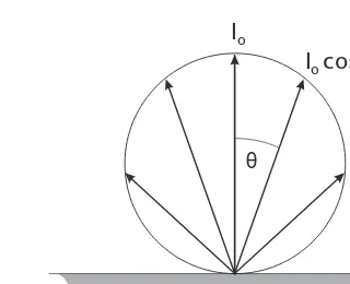
Lambert’s cosine law. Radiant intensity emitted from extended
sur-faces is usually not evenly distributed in angle. A very important rela-tion for perfect emitters, or perfect receivers, isLambert’s cosine law. A surface is calledLambertian if its radiance is independent of view angle, that is, L(x,θ,φ) =L(x). The angular distribution of radiant intensity can be computed directly from Eq. (2.18):
I(θ)=cosθ
S
L(x)dS=I0cosθ (2.23)
It is independent of angleφ and shows a cosine dependence on the angle of incidenceθas illustrated in Fig.2.8. The exitance of a planar Lambertian surface is derived from Eq. (2.14), pullingLoutside of the angular integrals
M(x)=L(x)
2π
0
π/2
0