JEJAK
Journal of Economics and Policy http://journal.unnes.ac.id/nju/index.php/jejak
WORLD OIL PRICE IMPACT ON INTEREST RATE AND
UNEMPLOYMENT: EVIDENCE FROM EURO
Husnirokhim N. Alim
Ministry of Public Works and Public Housing the Republic of Indonesia
Permalink/DOI: http://dx.doi.org/10.15294/jejak.v7i1.3838
Received: 4 September 2013; Accepted: 26 Oktober 2013; Published: Maret 2014
Abstract
Notable increases in the world price of oil have been generally recognized implies economic activities and macroeconomic policies. This paper tries to analyze the oil price and macroeconomic policy relationship by means of analyzing the impact of oil prices on real interest rate and unemployment. This paper tests these relationships in Europe Area Countries using annual data from 1970 to 2009 by using AWM database. Innovation or shock in world price of oil will affect the real interest rate and unemployment from initial period and fade away in very long time horizon.
Keywords: world price of oil, interest rate, unemployment, Euro zone
Abstrak
Tingginya harga minyak dunia telah dipercaya sebagai faktor yang mempengaruhi aktifitas ekonomi dan kebijakan makroekonomi. Penelitian ini bertujuan untuk menganalisis hubungan antara harga minyak dan kebijakan makroekonomi dengan menganalisis dampak harga minyak pada tingkat bunga riil dan pengangguran. Studi ini menguji hubungan tersebut di negara-negara Eropa dengan menggunakan data tahunan mulai tahun 1970- 2009 dengan database AWM. Inovasi dan tingginya harga minta akan mempengaruhi suku bunga riil dan pengangguran mulai dari periode awal dan berakhir dalam jangka waktu yang lama.
Kata Kunci: harga minyak dunia, suku bunga, pengangguran, zona Euro
How to Cite: Alim, H. (2014). Dampak LNG Academy Terhadap Kesiapan Tenaga Kerja Baru di Badak LNG. JEJAK Journal of Economics and Policy, 7 (1): 1-13 doi: 10.15294/jejak.v7i1.3838
© 2014 Semarang State University. All rights reserved
Corresponding author :
Address: Jalan Patimura No 20 Kebayoran Baru Jakarta Selatan E-mail: h.n.alim@alumnus.rug.nl
INTRODUTION
Oil unquestionable becomes important part of the economy because of its function as an “economic lubricants”. Its price, however, fluctuates and affects the world-wide economy. Based on historical series, oil price faces a bumpy pattern from 19th century.
During period 1862-1864 was became the first oil shock. The onset of the U.S. Civil War brought about a surge in prices and commodity demands generally. According to Cunado and Gracia (2003), prices of oil continue to rise dramatically since the World War II. During the period 1960–1999, there were four notably oil shocks: first period was in 1973–1974, when the Organization of Petroleum Exporting Countries first imposed an oil embargo and then greatly increased world crude oil prices from $3.4 to $13.4 per barrel. Secondly, in 1978–1979, after the Iranian revolution disrupted oil supplies, the price rose from $20 to $30 per barrel. The following shock was in 1990 in accordance with the Iraq’s invasion of Kuwait. At this period the price went from $16 to $26 per barrel. The fourth was in 1999 when the prices have grown up from $12 to $24 per barrel.
In the early 21st century, the fluc-tuation was continued. The price climbed in 2002 due to production cutting of oil in Venezuela and second Persian Gulf War; when the U.S. attacks on Iraq. These would both be characterized as exogenous geopo-litical events. During 2007-2008 increase of oil price was generated by growing economic demand and stagnant supply. The IMF estimated real gross world product grew at an average annual rate of 4.7%and world oil consumption grew 3% per year. These strong demand pressures were the key reason for the steady increase in the price of oil over
this period, though there was initially enough excess capacity to keep production growing along with demand (Hamilton, 2013).
Perhaps more than hundreds of empi-rical studies find that oil price exacerbates the macroeconomic activities in net oil-importing countries through the demand-side (income transfer) and supply-demand-side (production cost) channels. From the demand side analyses, Ferderer (1996) states the oil shock can lower aggregate demand due to the price rise redistributes income from the net oil importers to exporters. Brown and Yucel (2002) mention that if consumers expect the rise in oil prices to be temporary, or if they expect the short term effects on output to be greater than the long-term effects, they will enable to manage their consumption level by saving less or borrowing more which boosts the equilibrium real interest rate. With slowing output growth and an increase in the real interest rate, the demand for real cash balances falls, and for a given rate of growth in the monetary aggregate, the rate of inflation increases. Therefore, rising oil prices reduce GDP growth and boost real interest rates and the measured rate of inflation (Ito, 2010)
lead to increased unemployment and a further reduction in GDP growth. The reduction in GDP growth is accompanied by a reduction in labor productivity. Unless real wages fall by as much as the reduction in labor productivity, firms will lay off workers, which will generate increased unemploy-ment and further GDP losses. Ahmad (2013). If wages are nominally sticky downward, the only mechanism through which the neces-sary wage reduction can occur is through unexpected inflation that is at least as great as the reduction in GDP growth.
Cunado and Gracia (2003), which ana-lyze oil price impact on inflation in European countries, show that oil price has permanent effects on inflation. Furthermore, significant differences are found among the responses of the countries to these shocks. Another important thing is that the effect of oil prices on growth is asymmetric. Although a rise in oil price has a significant negative effect on growth, a fall in oil price does not cause an economic expansion (Cunado and Gracia, 2003, Hamilton, 2013, and Abeysinghe, 2001).
Empirical evidence impact of oil price that covering Asian countries conducted by Cunado and Gracia (2005). They suggest that oil prices have a significant effect on both economic activity and price indexes, although the impact is limited to the short run and more significant when oil price shocks are defined in local currencies. Abeysinghe (2001) reveals the identical result, however the transmission effect of oil prices on growth may not be that important for a large economy like the US but it could play a critical role in small open economies such as in Asian.
Dogrul and Soytas (2010) analyze unemployment rate and two input prices, namely energy (crude oil) and capital (real interest rate) in an emerging market, Turkey,
for the period 2005:01–2009:08. By using Structural Vector-Autoregrresion, they find the real world price of oil and interest rate improve the forecasts of unemployment in the long run. This finding supports the hypothesis that labor is a substitute factor of production for capital and energy.
The latest studies reveal that the impact of hiking price of oil not brings huge impact on macroeconomic indicators. Schmidt and Zimmermann (2005) and Schmidt and Zimmermann (2007) take study in Germany economy why the effects of oil price shocks on the German economy have reduced. They show that the oil intensity of production was reduced since the oil price-shocks of the seventies and early eighties. In this case oil prices would have become of minor importance for business cycle analysis. Loscheland Oberndorfer (2009) take further specific analyses impact of oil price on unemployment in Germany by using monthly data from 1973 to 2008. The result confirms those two prior studies; although volatility of oil price impacts still affect unemployment in Germany, the effects is weakened in Germany especially after 1980s when the economy getting efficient in using energy.
wide range aggregation of macroeconomic time-series of sixteen countries in Euro area.
The plan of the paper is as follows. First of all I briefly present the overview of price of oil condition across the centuries. Secondly, I discuss some empirical evidence that can link the fluctuation of oil price-macroeco-nomic indicators and also provide metho-dology and data selection that will be employed. Thirdly, methodology and data selection will be explained briefly. In the main part of this paper, I analyze the impact of oil price toward unemployment and interest rate in euro area. Finally, the last part will provides some concluding remarks.
METHODOLOGY AND DATA SELECTION
In order to find the relationship among oil price and macroeconomic variables, this paper will use a structural VAR model (SVAR). SVARessentially employs economic theory to sort out the contemporaneous links among the variables. This method requires identifying assumptions that allow correla-tion to be interpreted causally (Stock and Watson, 2011). Standard practice in VAR analysis is to report output from Granger-causality tests, impulse responses, and forecast error variance decompositions. Stock and Watson (2011) explain that Granger-causality evaluate whether the lagged values of a variable can predict other variables. Impulse response function can be applied to trace out the response of current and future values of each variables to a one-unit increase in the current value of one of the VAR errors, assuming that this error will return to zero in subsequent periods and that all other errors are equal to zero. The last thing to be noted, VAR provides forecast error decomposition which is the percentage of the variance of the error made in forecasting a variable due to a specific shock at a certain period.
This paper focuses on impact of oil price on two macroeconomics indicators namely real interest rate and unemployment. The world oil price variable measured in real term rather than in nominal term to get rid from world inflation bias and also adjusted in Euro rather than US Dollar. This specifi-cation is based on Abeysinghe (2001) specification.
Nominal world oil price; WGDPDEFt: World
GDP deflator; ERt: Euro per US$ exchange
rate
Interest rate is converted into real term as well.
REALIRt = NIRt – HICPt (2)
REALIRt: Real interest rate in Europe (%);
NIRt: Nominal short term interest rate ;
HICPt: Overall Harmonized Index of
Consumer Prices; Unemployment (LUNNt) is
in logarithmic number of unemployment in period t.
RESULT AND DISCUSSION
First step to make SVAR model, we have to make sure that all those variables are stationer1. One of the methods is by applying Augmented Dickey-Fuller unit root test. From Table 1 we can conclude that not all variables are stationer in level but they are stationer in first different (using intercept or using intercept & trend).
1
It is important to note that through residual test, our data have no auto-correlation, not normally distributed, and homoscedasticity (See Appendix 1, 2, and 3). After all variables are stationer in the same level, we can specify the maximum lag. In our case, optimum lag length k is determined
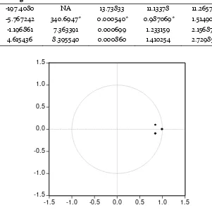
to be 1 by final prediction error (FPE), likelihood ratio test (LR), Akaike info criterion (AIC), Schwarz information criterion (SIC) and Hannan-Quinn (HQ) (Table 2) and all the inverse roots are inside the circle (Figure 1).
Table 1. Augmented Dickey-Fuller Unit Root Test
ADF test in Level
ADF test in 1st Different
Variables t-statistics Variables t-statistics
Intercept loil -2.1904 Intercept Loil -6.698*
realir -1.4282 Realer -4.3693*
lunn -2.9194** Lunn -3.2060**
Intercept & Trend loil -2.1518 Intercept & Trend Loil -6.6066*
realir -2.3774 Realer -4.4304*
lunn -2.1133 Lunn 3.6795**
Note: *) statistically significant at α 1% **) statistically significant at α 5% ***) statistically significant at α 10%
Table 2. Lag Length Specification
Lag LogL LR FPE AIC SC HQ 0 -197.4080 NA 13.73833 11.13378 11.26574 11.17984
1 -5.767242 340.6947* 0.000540* 0.987069* 1.514909* 1.171299*
2 -1.196861 7.363391 0.000699 1.233159 2.156878 1.555562
3 4.615436 8.395540 0.000860 1.410254 2.729853 1.870829
-1.5 -1.0 -0.5 0.0 0.5 1.0 1.5
-1.5 -1.0 -0.5 0.0 0.5 1.0 1.5
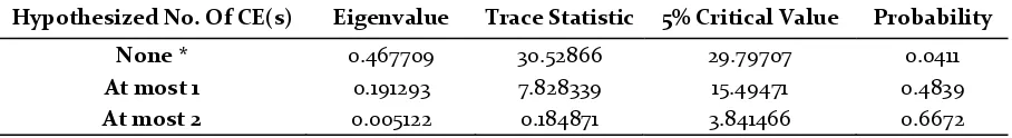
Table 3. Johansen Cointegration Test
Hypothesized No. Of CE(s) Eigenvalue Trace Statistic 5% Critical Value Probability
None * 0.467709 30.52866 29.79707 0.0411
At most 1 0.191293 7.828339 15.49471 0.4839
At most 2 0.005122 0.184871 3.841466 0.6672
Although all variables are stationer in first different, we can still apply SVAR in level since our model is cointegrated2. It has been tested using Johansen Cointegration test (Table 3). The procedure involves a SVAR in levels make us not loss of information due to differencing. SVAR model in this paper as follow:
Vt
vector of constants, β1 is (3×3) coefficient
matrices, and εVt denotes white noise
residuals. In our case, optimum lag length k
is determined to be 1.
Long Run Granger Causality and Genera-lized Impulse Responses
The Granger causality framework allows for testing the existence and the direction of causality between variables (table 4).
We observe that there are only some variables have Granger causality. Lag value of price of oil and unemployment can signifi-cantly, individually or together, help to predict real interest rate. Lag price of oil also can predict unemployment whereas real interest rate does not. These results generally confirm what Dogrul and Soytas (2010) did in Turky case. Therefore the real world price of
2
Wooldridge (2013) states cointegration applies when two series are stationer in first different, but a linear combinationof them is in level. This kind of regression is not spurious, buttells something about the long-run relationship between them.
oil and interest rate improve the forecasts of unemployment in the long run.
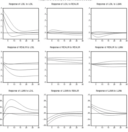
Now we are in position to explain how the responses of unemployment, oil price and interest rate toone standard deviation shocks to other variables in the SVAR. Impulse response function (Figure 2) explains shock in oil price increases the real interest rate and the impact tends to stand still even until 30 years. Shock on real interest rate leads to negative response on unemployment and fades away after 17 years. Shock in oil price initially gives negative impact on unemployment. Nevertheless, it gradually brings positive impact after 2 years, reaches the peak at seventh years after, and slightly fades away. Those means that oil price fluctuation bring huge impact toward real interest rate and unemployment.
Table 4. Granger Causality Test
From To test statistics p-value
REALIR LOIL 0.565138 0.4522
LUNN LOIL 1.464788 0.2262
REALIR and LUNN LOIL 1.684591 0.4307
LOIL REALIR 9.103531 0.0026*
LUNN REALIR 3.171558 0.0749***
LOIL and LUNN REALIR 14.12472 0.0009*
LOIL LUNN 6.948099 0.0084*
REALIR LUNN 0.120640 0.7283
LOIL and REALIR LUNN 7.427383 0.0244**
*) statistically significant at α 1%; **) statistically significant at α 10%
Response of LOIL to LOIL
-.1
Response of LOIL to REALIR
-.1
Response of LOIL to LUNN
-6
Response of REALIR to LOIL
-6
Response of REALIR to REALIR
-6
Response of REALIR to LUNN
.08
Response of LUNN to LOIL
-.08
Response of LUNN to REALIR
-.08
Response of LUNN to LUNN Response to Cholesky One S.D. Innovations ± 2 S.E.
0
V ariance Decomposition of LOIL
0
V ariance Decomposition of REA LIR
0
V ariance Decomposition of LUNN
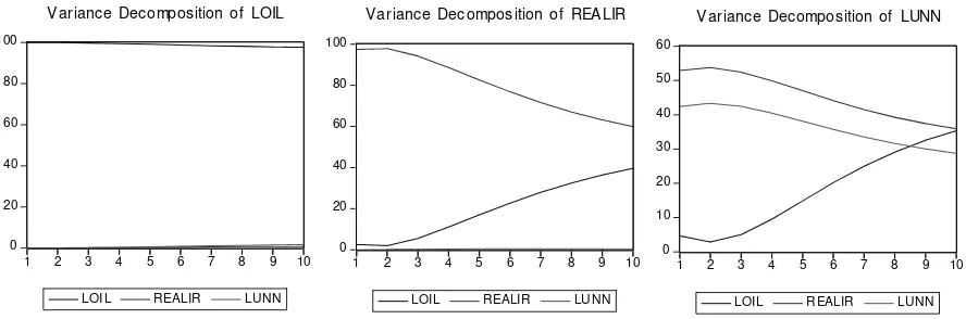
Figure 3. Variance decomposition
CONCLUSION
A lot of researches have been done to find relation of hiking oil price and some macroeconomic indicators. Here we present the effect of oil price toward two funda-mental macroeconomic indicators from supply side; real interest rate and unemploy-ment in aggregate euro area. We use help SVAR method to prove it.
We find that innovation or shock in world price of oil will affect the real interest rate and unemployment from initial period and fade away in very long time horizon. Our findings in euro area confirm what have been suggested by previous researcher that shock in world oil price will affect on unemploy-ment as well as real interest rate.
The weakness from this research is data limitation since AWM only provide annually data that make it difficult to split data to differentiate period before and after 1980 in order to see the exact effect of efficient energy using like what have Loschel and Oberndorfer (2009), Schmidt and Zimmermann (2005) and Schmidt and Zimmermann (2007) been done in Germany case.
REFERENCES
Abeysinghe, Tilak. (2001). Estimation of Direct and Indirect Impact of Oil Price on Growth,
Economics Letters, 73 (2001), 147–153.
Ahmad, Fawad. (2013). The Effect of Oil Prices on Unemployment: Evidence from Pakistan. Busi-ness and Economics Research Journal Volume 4 Number 1 2013 pp. 43-57 ISSN: 1309-2448. Brown, Stephem P.A., and Yucel Mine K. (2002).
Energy Prices and Aggregate Economic Activity: an Interpretative Survey, The Quarterly Review of Economics and Finance, 42 (2002), 193–208. Cologni, Alessandro., and Manere Matteo. (2008). Oil
Prices, Inflation and Interest Rates in a Structural Cointegrated VAR Model for the G-7 Countries, Energy Economics, 30 (2008), 856– 888.
Cunado, Juncal., and Gracia Fernando Perez de. (2003). Do Oil Price Shocks Matters? Evidence for Some European Countries, Energy Economics, 25 (2003), 137–154
Cunado, J., and Gracia F. Perez . (2005). Oil Price, Economic Activity and Inflation: Evidence for some Asian Countries, The Quarterly Review of Economics and Finance, Vol 45, pp 65-83.
Dogrul, H. Gunsel., and Soytas Ugur. (2010). Relationship between Oil Prices, Interest Rate, and Unemployment: Evidence from an Emerging Market, Energy Economics, 32 (2010), 1523–1528. Ferderer, J. Peter . (1996). Oil Price Volatility and the
Hamilton, James D. (2013). Historical Oil Shocks,
Handbook of Major Events in Economic History, Routledge, pp. 239-265.
Ito, Katsuya .(2010). The Impact of Oil Price Volatility on Macroeconomic Activity in Russia, Economic Analysis Working Papers, 9th Volume – Number 05.
Loscheland, Andreas., and Oberndorfer Ulrich. (2009). Oil and Unemployment in Germany, Discussion Paper Centre for European Economic Research,No 08-136.
Schmidt, T., and Zimmermann T. (2005). Effects of Oil Price Shocks on German Business Cycles, RWI: Discussion Papers, No. 31, Essen.
Schmidt, T., and Zimmermann T. (2007), Why are the Effects of Recent Oil Price Shocks so Small?,Ruhr Economic Paper, No. 21, Essens. Spencer, David E. (1989). Does Money Matter? The
Robustness of Evidence from Vector Autore-gressions, Journal of Money, Credit and Banking, Vol. 21, No. 4, pp. 442-454.
Stock, James. H., and Watson Mark W.(2011). Vector Autoregressions, Journal of Economic Perspec-tives, Vol. 15 No. 4 101-115
APPENDIX
(E-views output)
Appendix 1: LM Test
VAR Residual Serial Correlation LM Tests
Null Hypothesis: no serial correlation at lag order h Date: 01/03/14 Time: 20:39
Sample: 1970 2009 Included observations: 38
Lags LM-Stat Prob
1 7.821475 0.5522 2 7.211241 0.6151 3 14.43492 0.1077 4 6.817196 0.6561 5 10.44691 0.3155 6 11.47532 0.2445 7 9.103428 0.4278 8 10.39309 0.3196 9 9.525184 0.3903 10 3.493471 0.9415 11 9.428591 0.3987 12 6.026257 0.7373 Probs from chi-square with 9 df.
Appendix 2: Normality Test
VAR Residual Normality Tests
Orthogonalization: Cholesky (Lutkepohl)
Null Hypothesis: residuals are multivariate normal Date: 01/03/14 Time: 20:39
Sample: 1970 2009 Included observations: 38
Component Skewness Chi-sq df Prob. 1 0.029311 0.005441 1 0.9412 2 -0.277787 0.488717 1 0.4845 3 0.738059 3.449960 1 0.0633
Joint 3.944118 3 0.2676
Component Kurtosis Chi-sq df Prob. 1 2.749111 0.099663 1 0.7522 2 2.451942 0.475583 1 0.4904 3 3.114838 0.020881 1 0.8851
Joint 0.596127 3 0.8973
Appendix 3: Heteoskedasticity Test
VAR Residual Heteroskedasticity Tests: No Cross Terms (only levels and squares)
Date: 01/03/14 Time: 20:40 Sample: 1970 2009
Included observations: 38 Joint test:
Chi-sq df Prob. 52.01015 36 0.0410
Individual components:
Dependent R-squared F(6,31) Prob. Chi-sq(6) res1*res1 0.134543 0.803206 0.5751 5.112641 res2*res2 0.190013 1.212033 0.3266 7.220478 res3*res3 0.260766 1.822553 0.1271 9.909119 res2*res1 0.162824 1.004871 0.4399 6.187293 res3*res1 0.114792 0.670001 0.6745 4.362084 res3*res2 0.193755 1.241642 0.3125 7.362693
Appendix 4: VAR Result
Vector Autoregression Estimates Date: 01/03/14 Time: 20:41 Sample (adjusted): 1972 2009
Included observations: 38 after adjustments Standard errors in ( ) & t-statistics in [ ]
LOIL REALIR LUNN
LOIL(-1) 0.802081 -1.508612 0.065207
(0.09949) (0.50000) (0.02474) [ 8.06209] [-3.01721] [ 2.63592]
REALIR(-1) -0.001965 0.978781 0.000226 (0.00261) (0.01314) (0.00065)
[-0.75176] [ 74.5140] [ 0.34733]
LUNN(-1) -0.198376 -1.467034 0.907148
(0.16391) (0.82377) (0.04076) [-1.21028] [-1.78089] [ 22.2578]
C 2.340304 13.83339 0.705927
(1.34267) (6.74794) (0.33386) [ 1.74302] [ 2.05002] [ 2.11445] R-squared 0.657749 0.998217 0.979439 Adj. R-squared 0.627551 0.998060 0.977625 Sum sq. resids 3.179669 80.31298 0.196593 S.E. equation 0.305810 1.536928 0.076041 F-statistic 21.78081 6345.031 539.8734 Log likelihood -6.784290 -68.13822 46.10020 Akaike AIC 0.567594 3.796748 -2.215800 Schwarz SC 0.739972 3.969126 -2.043423 Mean dependent 3.242326 -73.11547 9.195516 S.D. dependent 0.501093 34.89133 0.508349 Determinant resid covariance (dof adj.) 0.000528
Determinant resid covariance 0.000378
Log likelihood -12.03392
Appendix 5: Short Run Structural VAR Output
Structural VAR Estimates Date: 01/03/14 Time: 20:41 Sample (adjusted): 1972 2009
Included observations: 38 after adjustments
Estimation method: method of scoring (analytic derivatives) Convergence achieved after 10 iterations
Structural VAR is just-identified
Model: Ae = Bu where E[uu']=I
Restriction Type: short-run pattern matrix A =
1 0 0
C(1) 1 0 C(2) C(3) 1 B =
C(4) 0 0
0 C(5) 0
0 0 C(6)
Coefficient Std. Error z-Statistic Prob.
C(1) -0.805333 0.804751 -1.000724 0.3170
C(2) 0.024287 0.026615 0.912515 0.3615
C(3) 0.036465 0.005296 6.885693 0.0000
C(4) 0.305810 0.035079 8.717798 0.0000
C(5) 1.517067 0.174020 8.717798 0.0000
C(6) 0.049525 0.005681 8.717798 0.0000
Log likelihood -18.37378 Estimated A matrix:
1.000000 0.000000 0.000000 -0.805333 1.000000 0.000000 0.024287 0.036465 1.000000 Estimated B matrix:
Appendix 6: Long Run Structural VAR Output
Structural VAR Estimates Date: 01/03/14 Time: 20:41 Sample (adjusted): 1972 2009
Included observations: 38 after adjustments
Estimation method: method of scoring (analytic derivatives) Convergence achieved after 23 iterations
Structural VAR is just-identified
Model: Ae = Bu where E[uu']=I
Restriction Type: long-run pattern matrix Long-run response pattern:
C(1) 0 0 C(2) C(4) 0
C(3) C(5) C(6)
Coefficient Std. Error z-Statistic Prob.
C(1) 3.641434 0.417701 8.717798 0.0000
C(2) -387.4043 47.44902 -8.164642 0.0000
C(3) 1.626881 0.210137 7.742010 0.0000
C(4) 102.5306 11.76106 8.717798 0.0000
C(5) -0.509109 0.076951 -6.616001 0.0000
C(6) 0.308902 0.035433 8.717798 0.0000
Log likelihood -18.37378 Estimated A matrix:
1.000000 0.000000 0.000000 0.000000 1.000000 0.000000 0.000000 0.000000 1.000000 Estimated B matrix: