OWN PRICE AND THE SUPPLY CURVE

3

Supply

C O N C E P T S

● Determinants of Supply ● Supply Schedule

● Supply Curve ● Supply Function

● Business Taxes ● Hoarding

● Change in Quantity Supplied versus Change in Supply ● Market Supply

● Price Elasticity of Supply ● Arc Elasticity of Supply

● Point Elasticity of Supply

W

hile consumers or households demand goods and services, it is the producers or firms who supply them. In this chapter we analyse what factors determine the supply of a particular good to a market within a given time period.

As an example, suppose that you have a factory in Chennai that produces foot-ball. What factors determine how many footballs you produce and supply to the market in a span of, say, a year?

One is the market price of a football itself (assuming that all footballs are exactly of the same size and quality). All else the same, if the market price of foot-ball increases, you would tend to supply more.

Another factor is the cost of raw materials, labour and so on that go into the production of footballs. If the leather and other synthetic material with which a football is made become more expensive, it is a less profitable business and you would produce less.

Technology also matters. If you find a more efficient way of combining labour, machines and raw materials in producing football, you would produce more.

Still another factor is the price of substitute goods in production. Suppose your factory makes volleyballs as well, and to our pleasant surprise, India wins a silver medal in women’s volley ball. Volleyball will now be in great demand among women and men in sport and the price of volleyballs will rise. How would this affect your supply of footballs? It would decline, as you would divert more of your productive resources from football to volleyball.

It is now time to state these factors of supply generally and consider their impli-cations.

OWN PRICE AND THE SUPPLY CURVE

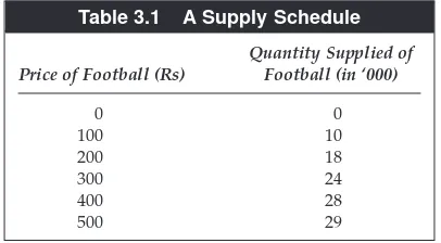
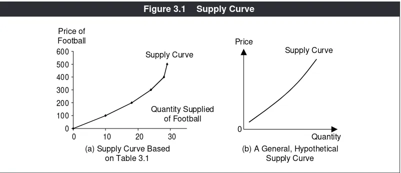
All other things remaining the same, the higher the price of a product, the more a firm will produce and supply to the market. This is the law of supply, analogous to the law of demand. Table 3.1 lists various quantities of football supplied at dif-ferent prices. Such a table describes a supply schedule. Figure 3.1(a) graphs this table, measuring price and quantity along the y-axis and the x-axis respectively.

Table 3.1 A Supply Schedule

Quantity Supplied of Price of Football (Rs) Football (in ‘000)

0 0

100 10

200 18

300 24

400 28

The resulting curve is a supply curve, a graphical representation of the law of sup-ply or a supsup-ply schedule. It is upward sloping or positively sloped because a higher quantity of supply is associated with a higher price. Figure 3.1(b) draws a smooth supply curve for analytical purposes.

SHIFTS OF A SUPPLY CURVE

Similar to the case of demand, factors other than the own price can cause a shift in a supply curve.

Input Prices

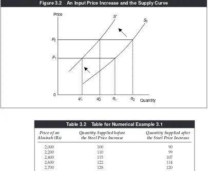
Consider Figure 3.2, in which S₀is the original supply curve. At the price p₁, the quantity supplied is q₁; at p₂, the quantity supplied is q₂and so on. Now suppose there is an increase in the price of an input or in the prices of several inputs that are used in making the product. This will raise costs. As this reduces profitability, at any given price, a firm will supply less. At p₁, the quantity supplied now is q′₁, which is less than q₁, at p₂, it is q′₂and so on. The resulting supply curve is S’, lying to the left of S₀. Hence, an increase (or a decrease) in input prices shifts a supply curve to the left (or right).

NUMERICAL EXAMPLE 3.1

A company produces steel almirahs of a given type, dimension and quality. The market price of steel rises by 20 per cent. Through a numerical example, illustrate how this would affect the company’s supply curve of almirahs.

An increase in the price of steel reflects an input price increase. This will imply that at the same price for an almirah, the company will supply less. Table 3.2 offers

0 100 200 300 400 500 600

0 10 20 30

Price of Football

Quantity Supplied of Football

Supply Curve

(b) A General, Hypothetical Supply Curve Price

Supply Curve

Quantity 0

(a) Supply Curve Based on Table 3.1

an example. Column 2 enumerates the original quantities supplied at various prices. In column 3 each entry is less than the corresponding entry in column 2, meaning a decrease in the quantities at each price. Thus, in relation to column 2, column 3 illustrates the increase in the price of steel. We can verify that the graph-ical plot of column 3 against the price column lies to the left of that of column 2, representing a leftward shift of the supply curve as shown in Figure 3.2.

Technology

As discussed earlier, a technological improvement will induce a producer to supply more at any given price (the opposite of what happens when input prices increase). Thus it will shift a supply curve to the right, as illustrated in Figure 3.3. The old sup-ply curve is S

0and the new one after the technological improvement is S1.

Quantity Price

0

S′

p₂

p₁

q′1 q′2 q1 q2

S₀

Figure 3.2 An Input Price Increase and the Supply Curve

Table 3.2 Table for Numerical Example 3.1

Price of an Quantity Supplied before Quantity Supplied after Almirah (Rs) the Steel Price Increase the Steel Price Increase

2,000 100 90

2,200 110 99

2,400 115 107

2,600 122 114

2,700 128 120

Price of a Substitute Good in Production

In our football-volleyball example, an increase in the price of volleyball led to a decrease in the production of football. Generalising from this, we can say that an increase in the price of a substitute good in production will shift the supply curve of a given product to the left. This is illustrated in Figure 3.4. The original supply curve is S

0, whereas the new supply curve is S1.

Business Taxes

Businesses not only incur the cost of production, but also pay a variety of taxes because of their production activity. For example, there are excise taxes (see Clip 3.1

Price

Quantity

S₁

0

S₀

Figure 3.3 Technological Improvement and the Supply Curve

Price

Quantity

S₁

0

S₀

for a brief discussion of these taxes). If a business buys inputs from abroad, it may have to pay a customs duty. If it is a service, then a service tax has to be paid.1 Starting in the financial year 2005–06, many states use VAT (Value Added Tax).2

All these taxes that businesses pay can be understood as some tax on output and we can, in general, call them ‘business taxes.’ If such taxes increase, from a producer’s point of view, it is like an increase in the price of an input. Thus, an increase (or a decrease) in business taxes shifts the supply curve to the left (or right).

Other Factors

Other factors affect the supply curve of a product as well. For the production of an agricultural good, weather plays an important role. We all know how depend-ent our agricultural output is on the monsoons.

Another factor is price speculation which is same as future price expectation. If it is speculated that the price of a good will rise in the near future because of an external factor, suppliers may engage in product hoarding by not releasing the good to the market. They do so because they expect to make larger profits later by releasing the output when the market price is much higher. Hoarding behaviour tends to reduce the current supply of the product, that is, it tends to shift the cur-rent supply curve to the left. This happens typically in case of essential goods dur-ing emergencies like a war, flood or drought. In the same vein, if suppliers perceive that the price of the good is expected to fall in the future, they would tend to supply more to the market now. In general, an increase (or a decrease) in the expected future price would decrease (or increase) the current supply of a com-modity to the market and, therefore, shift the supply curve to the left (or right).

Clip 3.1: Excise Taxes in India

Excise taxes are levied mostly by the central government for the sake of rais-ing revenues. It varies from one sector to another. Some sectors may be exempt from this tax. For instance, in 2002–2003, producing kerosene carried an excise duty/tax of 16 per cent; for tea it was Re 1 per kilogram. In 2003–04, the excise duty rates on garments, passenger cars and computers stood at 10, 24 and 8 per cent respectively, down from 12, 32 and 16 per cent respectively in the previous financial year. State governments also impose excise duties but on a very limited number of products, mostly alcoholic.

1_{Service tax is a relatively new concept. It has been in existence since the mid-nineties only. Over time, the service tax rate}

has been increasing. In the financial year 2005–06, it was set at 10.2%.

2_{A VAT effectively means that businesses do not have to pay tax on inputs purchased from other sectors; taxes are paid}

MARKET SUPPLY CURVE

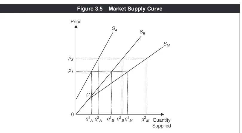
So far, we have discussed the supply curve of a single producer. For the entire industry we can talk about the market supply curve, analogous to the market demand curve. If there are 50 producers in a market, for example, the market sup-ply curve is the horizontal summation of the supsup-ply curves of these 50 producers. What are the determinants of the market supply curve? The answer is: all factors that affect the individual supply curve plus the number of firms.

For illustration, Figure 3.5 assumes two firms in the market, A and B. Their respective supply curves are indicated as S_A and S_B.At the price p₁, firm A and firm B respectively supply the quantities, q1

Aand q1B. The total quantity supplied in the market is equal to q1

A+q1B≡ q1M. Similarly, at the price p2, the individual quan-tities supplied are q2

Aand q2B. Hence the total quantity supplied equals q2A+q2B≡ q2M. If we join the price-quantity combinations like (p₁, q1

M), (p2, q2M) and so on, we obtain the market supply curve, shown as the curve 0CS_M.

CHANGE IN QUANTITY SUPPLIED VERSUS CHANGE IN SUPPLY

The distinction is similar to that between a change in quantity demanded and a change in demand. Change in quantity supplied refers to a movement along a given supply curve and this occurs because of a change in the own price. In con-trast, a change in supply refers to a shift of an entire supply curve. For instance, a change in technology changes the supply.

Quantity Supplied Price

p₂

S_A

S_B

S_M

p₁

q1

Aq2A q1B q2Bq1M q2M

0

C

Essentially these terms distinguish the effect of own price on the supply of a good from the effects of other determinants.

ELASTICITY

Parallel to demand, elasticity of supply measures the responsiveness of quantity supplied. The price elasticity of supplyis defined by:

(3.1)

This is the percentage formula. The numerator is equal to (Δqs/qs) ×100, where Δ

denotes the change and q_sdenotes the quantity supplied. Similarly, the

denomin-ator equals (Δp/p) ×100, where pdenotes price. Hence, the percentage formula

can be alternatively expressed as:

(3.2)

Arc Elasticity

For any change in price which is not very small, e_sis sensitive to an interchange

between the original price and the new price and the corresponding interchange between the original quantity and the new quantity. This problem is avoided by using the arc elasticity of supplydefined by:

(3.3)

where (p₀, q₀) is the old price-quantity pair and (p₁, q₁) the new one. This is

analo-gous to the arc elasticity of demand.

NUMERICAL EXAMPLE 3.2

A sugar manufacturer was supplying 10 quintals of sugar to the market when sugar was selling for Rs 10 per kg. The price of sugar has increased to Rs 14 per kg and the manufacturer is supplying 15 quintals to the market. What is the arc elas-ticity of supply?

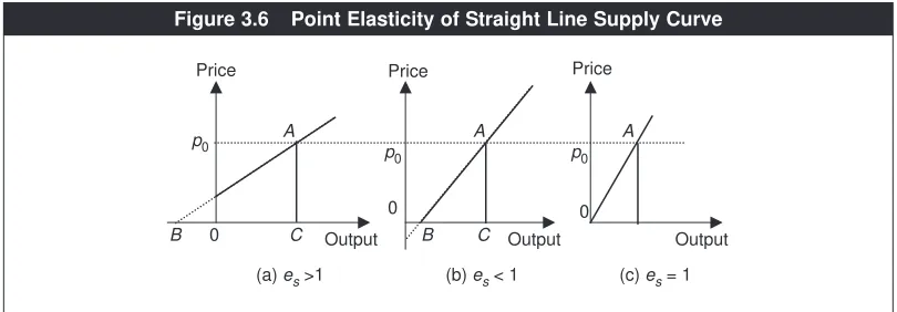
Point Elasticity of Supply

For a very small change in price, there is also a point elasticitymethod. Suppose the supply curve is a straight line. Figure 3.6 shows three possibilities. The supply line intersects the price axis first, the quantity axis first or the origin as shown in panels (a), (b) and (c) respectively. As proven in Appendix 3A, in panels (a) and (b), the point elasticity is equal to BC_/0C_{, the ratio of the horizontal segment to the}

quantity supplied. In panel (a) BC _>0C_{and hence} BC_/0C_{>1, that is, the point}

elasticity of supply is greater than one, or the supply is said to be elastic. In panel (b) it is the opposite: BC_/0C_{<1. The point elasticity is less than one or}

sup-ply is inelastic.

Panel (c) can be thought of as a special case, where the point B_{coincides with the}

origin. Thus, BC₌₀C_and e

s= 1. In other words, a straight line supply curve

pass-ing through the origin always has price elasticity equal to one (or ‘unitarily elastic’), regardless of how flat or steep the supply curve is. For instance, in Figure 3.7, all the three supply curves, S

1, S2and S3, have es =1 at any price.

There are two special cases of straight-line supply curves: one where it is verti-cal and the other where it is horizontal. These are shown in Figure 3.8. A vertiverti-cal supply curve has e

s=0, since the quantity supplied is fixed. Typically, this holds

when we look at the supply of a product at a given instant of time. For example, during a particular day, the supply of fish in the entire market of Kolkata is fixed. Assuming that fish cannot be stored, that amount of fish has to be sold in the mar-ket that day irrespective of how much price it fetches.3_{Along a horizontal supply}

curve, e

s= ∞, meaning that a little or a ‘marginal’ change in price will lead to an

arbitrarily large change in supply.

If the supply curve is not a straight line, the point elasticity at a given price depends on the slope of or the tangent to the supply curve at that price. If this tan-gent intersects the price axis first, then, as in Figure 3.6(a), the elasticity exceeds

Output Output

Figure 3.6 Point Elasticity of Straight Line Supply Curve

one. If it intersects the quantity axis first or the origin, it is less than or equal to one respectively. In Figure 3.9, for instance, at price p₀, the tangent intersects the quan-tity axis and, therefore, the price elasticity of supply is less than one.

How do we compare elasticities of two supply curves? Of course, if they are straight lines passing through the origin, we know that they will both have elas-ticity equal to one. We also know that if one (straight line) supply curve has the intercept on the price axis and the other on the quantity axis, the elasticity along the former is greater. But, barring these cases, we cannot compare in general except at their point of intersection. Turn to Figure 3.10. Just as in case of two inter-secting demand curves, at the price p₀, the flatter supply curve S_Bhas higher elas-ticity than the steeper supply curve S₁because the quantity adjustment due to a given price change is greater along the former. The reasoning is analogous to that

Output Price

0

S₁

S₂

S₃

Figure 3.7 Unitarily Elastic Supply Curves

Price

Supply Curve

Quantity Price

Supply Curve

Quantity

e_s= 0

behind the comparison shown in Figure 2.9 in Chapter 2. Thus, of two supply curves, the flatter supply curve is more elastic than the steeper supply curve at their point of intersection.

What about the elasticities of supply with respect to other factors like technol-ogy, input prices or taxes? In principle, one can define them. But there are several kinds of inputs and different types of technological improvements. Therefore, the standard practice is to not specify them as a general category. However, depend-ing on what we wish to analyse, we can always define and discuss the relevant elasticity of supply. For instance, if we are considering producers who are manu-facturing competing goods, we define a cross price elasticity of supply, for exam-ple, the elasticity of wheat production with respect to the price of sugar cane.

See Clip 3.2 for a sample of elasticities of supply. Output Price

C B

p₀

0

Supply Curve

A

Figure 3.9 Point Elasticity of a General Supply Curve

p₀

S_A

S_B

Output Price

0

More Elastic

Mathematically Speaking

The Supply Function

It is analogous to the mathematics of demand. Let q_A denote the output or the quantity supplied of good A, p_Aits price and p_Bthe price of a substitute good in production. Suppose there are three inputs: labour, capital and raw material. Let their prices be respectively w_L, w_Kand w_R.Finally, let Crepresent an index of the

Clip 3.2: Estimates of Elasticity of Supply

In general, compared to demand elasticities, supply elasticities are harder to estimate because of data availability problems and because firms operate in dif-ferent types of market environments. Yet, some estimates are available and the following table presents a sample. Notice that it contains own price elasticities of supply as well as examples of elasticities with respect to input price changes.

Elasticity of the With respect to

Supply of …… the Price of …… Study Estimate

Rice Own Chand (1998–99) 0.25 (India)

Wheat Own Chand (1998–99) 0.85 (India)

Oysters Own Muth, Anderson, 1.97: halfshell oysters

Karns, Murray and 2.30: shucked oysters Domanico (2000) 1.64: shellstock

oysters (US)

Broiler Poultry Own Fabiosa, Jenses 0.22 (Indonesia)

and Yan (2004)

Rice Fertiliser Chand −0.16 (India)

(an input) (1998–99)

Wheat Fertiliser Chand −0.02 (India)

(an input) (1998–99)

References

Chand, R. 1999. ‘Supply Responsiveness in India’s Rainfed Agriculture’, in the Annual Report 1998–99,the National Centre for Agricultural Economics and Policy Research. New Delhi: Indian Council of Agricultural Research.

Fabiosa, J. F., H. H. Jensen and D. Yan. 2004. ‘Output Supply and Input Demand System of Commercial and Backyard Poultry Producers in Indonesia’. Working Paper 04-WP 363, Center for Agriculture and Rural Development, Iowa State University.

level of technology or efficiency of production. We can then write a supply function for good Aas:

The law of supply implies that ∂_g

A/∂pA> 0. Substitutability of production implies

∂_g

A/∂pB < 0. An increase in the price of an input also has a negative effect on output.

Hence ∂_g

A/∂wL< 0, ∂gA/∂wK < 0 and ∂gA/∂wR < 0. A technology improvement

induces a firm to produce more. Therefore, ∂_g

A/∂C> 0.

If we are concerned only with changes in the own price, we can suppress other

variables and write the supply function as q_A=_g

A(pA). A linear function like

APPENDIX 3A: POINT ELASTICITY FORMULAS

Consider Figure 3.6. For a small price change from p₀,

E

E X

X E

E R

R C

C II S

S E

E S

S

3.1 A furniture manufacturer in Mumbai faces an increase in the price of teak wood. How will it affect the supply curve of furniture in the market? 3.2 Our furniture manufacturer has found a new mechanised way of polishing

furniture by which costs are reduced. Will this result in a change in the quantity supplied or a change in supply by the furniture manufacturer? Give reasons.

3.3 A farmer has some land, a part of which is used for growing wheat and the remaining for corn. Starting with a given supply curve of corn, if wheat begins to fetch a higher price in the market, how will the farmer’s supply curve of corn be affected and why?

3.4 Suppose the government reduces the excise duty imposed on a particular sector. How will this affect the supply curve?

3.5 A massive flood cuts off supplies of essentials like edible oil and onions to a particular region. All else the same, how would this affect the current sup-ply of edible oil by local sellers and why?

Economic Facts and Insights

● The quantity supplied of a product is dependent on own price, prices of

related goods in production, technology, input prices, business taxes and future price expectations.

● An increase in the own price tends to increase the quantity supplied of a

product.

● An increase in the price of a related good in production decreases the supply

the product in question.

● A technology improvement shifts the supply curve to the right, while an

increase in an input price shifts the supply curve of a product to the left. ● Business taxes like excise duties, VAT and service tax can be seen as a part

of the overall costs of production. Thus, an increase in the business taxes shifts the supply curve to the left.

● An increase in the expected future price of a product tends to reduce its

current supply.

● Market supply curve is the horizontal summation of the individual supply

curves.

● The price elasticity of supply measures the responsiveness of quantity

3.6 How will entries of foreign firms into a particular sector shift the individual supply curve of local firms as well as the market supply curve?

3.7 A local fisherman catches fish from a nearby river early in the morning and

sells all his catch by the same day (he does not have any storing facility). Consider his daily supply curve of fish to the market. Is it upward sloping, that is, will quantity supplied increase if there is an increase in the market price of fish?

3.8 ‘An increase in the market demand curve will shift the market supply curve

as well.’ Defend or refute.

3.9 A pencil manufacturer was supplying 400 dozen pencils when the price

was Rs 10. Now the market price has risen to Rs 14 and the manufacturer is supplying 420 dozen of pencils to the market. Calculate the arc elasticity of supply.

3.10 ‘Among two straight line supply curves, the steeper one is less price elastic.’ Comment.

3.11 A ladies-clothing manufacturer produces sari_{s and} shalwars_{. How will an}

increase in the average price of sari_{s affect the supply curve of} shalwar_s?