Does Birth Order Matter?
Joseph Price
a b s t r a c t
Using data from the American Time Use Survey, I find that a first-born child receives 20-30 more minutes of quality time each day with his or her parent than a second-born child of the same age from a similar family. The birth-order difference results from parents giving roughly equal time to each child at any point in time while the amount of parent-child quality time decreases as children get older. These results provide a plausible explanation for recent research showing a very significant effect of birth order on child outcomes.
I. Introduction
The extensive literature linking family size and child outcomes con-sistently reports that children in larger families have lower levels of educational at-tainment and worse outcomes in terms of risky behaviors and delinquency (Steelman et al. 2002). A recent surge in research has provided strong and consistent evidence of birth-order differences across a wide range of child outcomes, with children of higher birth orders (those who are born later) having worse outcomes. In fact, once birth order is controlled for, family size has either no effect or a very small effect on the first-born child (Black, Devereux, and Salvanes 2005; Conley and Glauber 2006; Gary-Bobo, Prieto, and Picard 2006).
Much less empirical research has been devoted to providing a plausible explana-tion for why children with a higher birth order have worse outcomes. Several factors might even point in the opposite direction since high-birth-order children generally experience a household environment in which the parents are more mature, more
Joseph Price is an assistant professor of economics at Brigham Young University. This paper has benefitted from helpful comments by Fran Blau, Keith Bryant, Janet Currie, Gordon Dahl, Rachel Dunifon, Ron Ehrenberg, Gary Fields, Jonathan Gruber, Robert Hernandez, George Jakubson, Robert Kaestner, Barrett Kirwan, Lars Lefgren, Dean Lillard, Albert Liu, Francesca Molinari, Liz Peters, Corinne Post, Mathis Schroeder, Gary Solon, Dan Rees, and participants at the NBER summer institute, APPAM, PAA, SOLE, and seminars at Cornell, Rochester, and the University of Oregon. The data used in this article can be obtained beginning August 2008 through July 2011 from Joseph Price, BYU Economics Department, 130 FOB, Provo, UT 84604 <joseph_ price@byu.edu>.
[Submitted September 2006; accepted February 2007]
ISSN 022-166X E-ISSN 1548-8004Ó2008 by the Board of Regents of the University of Wisconsin System
experienced at parenting, and have more income (Behrman and Taubman 1986; Powell and Steelman 1995). This paper examines one possible mechanism: the amount of time that a child spends with his or her parents. Parental time inputs are thought to be an important determinant of a child’s educational outcomes and presumably other outcomes as well. Thus, finding a connection between birth order and time spent with parents provides an important explanation for the link between birth order and child outcomes.
The analysis in this paper uses data from the American Time Use Survey (ATUS), which contains information on the amount of time each child in a household spent with one of his or her parents on a particular day, how the time was spent, and who else was present for the activity. Birth-order differences are estimated by match-ing each first-born child with a second-born child of the same age from a similar family. This cross-family comparison allows me to answer the question of whether a first-born child receives more quality time with his or her parents at a certain age than the younger sibling does when he or she reaches the same age.
The results in this paper show that in two-child families, the first-born child receives about 20 more minutes of quality father-time and 25 more minutes of quality mother-time each day at each age than the second-born child does at the same age. This leads to an aggregate difference of about 3,000 hours across the ages of 4–13.
The traditional intra-household allocation model of Becker and Tomes (1976) pos-its that parents allocate more human capital resources to the more able child so as to maximize the lifetime income of all children. Parents later use wealth transfers to equalize outcomes across children. Behrman, Pollak, and Taubman (1982) note that a parent’s allocation strategy can reinforce or compensate for ability differences, depending on the parent’s level of inequality aversion. This means that parents who have strong preferences for equity will allocate more time to the less able child. Within this framework, parents face a natural trade-off between equity and produc-tivity in terms of child outcomes. One assumption in each of these models is that parents purposefully allocate resources so as to maximize some parental utility func-tion (Behrman 1997).
The evidence in this paper shows, rather, that parents provide roughly equal time to each of their children at each point in time but spend less time with each child as their children get older. As a result, parents spend more time with the first-born child at each age than they do with the second-born child when he or she reaches the same age. Thus, the parents’ apparent desire for equity at each point in time actually leads to inequities in the total resources received by each child.
Past research asserts that a first-born child may have better outcomes because he or she gets to be an only child for the first few years of life (Hanushek 1992; Lindert 1977). The analysis in this paper is limited to years in which the second sibling is already present. This paper shows that the first-born child continues to get more time at each age even after additional siblings are born. The second-born child becomes the only child once the first-born child has left the home, but by this age, the amount of parent-child interaction is so much lower that it likely does not have as large an effect.
ages), the birth-order difference is much larger when the children are spaced further apart. I also find that fathers spend more quality time with sons than with daughters. As a result, the size of birth-order differences in time spent with one’s father is larger if the first child is a boy and is even larger if the second child is a girl.
The paper proceeds as follows. Section II discusses past research on the effects of birth order and parental time inputs on child outcomes. Section III describes the American Time Use Survey data used in the analysis. Section IV describes the em-pirical strategy and discusses the main results. Section V addresses the issues of incomplete fertility, sibling gender composition, birth spacing, and alternative meas-ures of parent-child interaction. Section VI simulates aggregate birth-order differences older than ages 4–13. Section VII concludes.
II. Birth Order, Parent Time Inputs, and Child Outcomes
Early studies in economics on birth-order differences in child out-comes generally found small or insignificant differences. Kessler (1991) and Hauser and Sewell (1983) find the effect of birth order to be insignificant, Behrman and Taubman (1986) provide some evidence of a positive effect of being first-born, and Hanushek (1992) finds a U-shaped relationship where the first- and last-born have the best outcomes. However, recently there has been a surge of research docu-menting strong and consistent birth-order differences, with higher-birth-order chil-dren having worse outcomes.
Black, Devereux, and Salvanes (2005) use administrative data for the entire pop-ulation of Norway over an extended period of time and find that lower-birth-order children (those born first) have higher levels of educational attainment, greater earn-ings, and (for women) a smaller likelihood of having a teenage pregnancy. In fact, the difference in educational attainment they find between a first- and fifth-born child is equivalent to the black-white gap in the United States.
Other recent papers that show that children with a lower birth order have more positive outcomes include Gary-Bobo, Prieto, and Picard (2006), Iacovou (2001), and Booth and Kee (2006) who look at educational outcomes; Aizer (2004) who looks at delinquent behaviors such as skipping school, using harmful substance, and hurting others; Gerner and Lillard (2006) who look at test scores; Conley and Glauber (2005) who look at being held back in school; and Argys et al. (2006) who look at risky behaviors such as substance abuse, sexual activity, and crime.
A major difficulty in posing a theoretical link between birth order and child out-comes is that the different theories provide opposing effects, leaving an ambiguous prediction as to the net effect. An alternative approach is to look for links between birth order and inputs that have been shown to influence positively child outcomes. One of these inputs is the amount of quality time a child spends interacting with his or her parent.
Unfortunately, providing a convincing causal link between parental time inputs and child outcomes has been an elusive search for researchers. In fact, it is difficult to imagine a natural experiment or policy change that would provide an exogenous shock to the amount of quality time provided to children and, at the same time, have no direct effect on child outcomes. Even with a plausible identification strategy, it is often difficult to get accurate measures of parental time inputs.1As a result, most past research has focused on maternal employment, with researchers asserting that weekly work hours are a good proxy for mother-child time. However, as noted by Blau and Grossberg (1992), mothers who work may compensate for the lack of total time by engaging in more developmental activities.
There are, however, many studies that provide a link between child outcomes and the frequency of certain activities, such as reading, playing, or eating dinner together. For example, Zick, Bryant, and Osterbacka (2001) find that children whose parents read or play with them more often have fewer behavioral problems and better grades. Other researchers that establish a link between reading to children and positive out-comes include Leibowitz (1977); Hill and O’Neill (1994); Snow, Burns, and Griffin (1998); and Se´ne´chal and LeFevre (2002). Studies that demonstrate a connection be-tween eating dinner as a family and wide range of child outcomes include Eisenberg et al. (2004) and Taveras et al. (2005).
In addition, Datcher-Loury (1988) finds that, after controlling for the mother’s work status, children whose mothers spend more time at home complete more years of schooling. Amato and Rivera (1999) find that children with more involved fathers are less likely to have behavioral problems, and Pleck (1997) reviews a number of studies and finds consistent evidence that indicates that higher levels of father in-volvement affect children in a positive way over a range of outcomes.
The primary focus of this paper is to analyze the empirical relationship between a child’s birth order and the amount of quality time spent with his or her parent. This relationship provides a potential explanation for the link between birth order and child outcomes found in other research. The results from this paper also provide in-sight about how parents allocate time to their children, which can be used when de-veloping theoretical models of parental decision making.
III. American Time Use Survey
The American Time Use Survey (ATUS), administered by the Bu-reau of Labor Statistics, is the first time that a federal statistical agency in the United
States has collected data on how people use their time. The survey began in January 2003, with 21,000 individuals completing the survey in 2003, 14,000 in 2004, and 13,000 in 2005. The survey will continue into the indefinite future with additional waves of data released each year.2
The respondents to the ATUS are sampled from the group of households in the outgoing rotation of the Current Population Survey. For each household, one adult (age 15+) is randomly selected to complete the survey. The respondent is asked to recount the activities of the previous day. For each activity, the respondent reports the starting and ending time, their location, and the members of their household who were present during the activity.
Since the ATUS respondents also participated in the Current Population Survey, I have detailed information about their marital status, labor status, and education level. The respondent is asked to provide the age, gender, and relationship to the re-spondent of each person in the household. This information makes it possible to con-struct measures of the child’s current family size, birth order, birth spacing, and gender composition of siblings.
The ATUS only surveys one parent in the family but the time use of other mem-bers of the family is observed as they come in contact with the respondent during the day. As a result, while the ATUS data does not provide information about how chil-dren use their time when they are not with their parents, it does give a very accurate measure of the time they spend with the parent participating in the survey and how this time is spent.
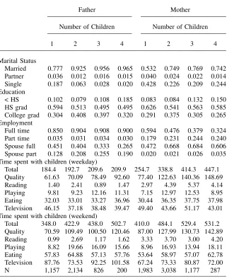
I use the ATUS coding of each activity to measure both the total amount of time the parent spends with their children as well as the amount of quality time. Quality time includes all activities in which either the child was the primary focus of the ac-tivity or in which there would be a reasonable amount of interaction, such as eating together.3Table 1 provides the average amount of time fathers and mothers spend with their children in terms of total time and quality time, along with time spent read-ing, playread-ing, eatread-ing, and watching television together.
I use the parent’s report on which children are present for each activity to deter-mine how much time each child spent interacting with his or her parent. This differs from most past studies that have looked at how much time parents spend with their children. Using the child as the unit of analysis makes it possible to look at within-family differences in quality time. Knowing who is present for each activity allows for classification of parent-child time by both the number of siblings and number of parents present during the activity.4
2. A more detailed description of the ATUS data is found in Hamermesh et al (2005). The data are publicly available at http://www.bls.gov/tus/home.htm.
3. Appendix Table A1 provides a list of the 13 activities that are included in the quality-time measure. Appendix Table A1 also reports the fraction of children who are engaged in each activity on the particular survey day, how much time was spent in the activity, and (for the two-child families) how much of that time was spent without the other sibling present. The last column indicates alternative cutoffs for quality time that I use as a robustness check in Section IV.
The analysis is limited to families with no more than four children in their house-hold. The identification strategy in this paper requires that I separate the analysis by family size and the number of families in the sample with more than four children is too small for meaningful statistical inference. The results in this paper, however, are still relevant for the majority of U.S. families.
The estimation strategy in this paper also requires that I have enough children of each birth order at a particular age to make a meaningful comparison. This is not
Table 1
Parent Characteristics and Time use by Number of Children
Father Mother
Number of Children Number of Children
1 2 3 4 1 2 3 4
Marital Status
Married 0.777 0.925 0.956 0.965 0.532 0.749 0.769 0.742
Partner 0.036 0.012 0.016 0.015 0.040 0.024 0.022 0.014
Single 0.187 0.063 0.028 0.020 0.428 0.226 0.209 0.244
Education
< HS 0.102 0.079 0.108 0.185 0.083 0.084 0.132 0.150
HS grad 0.594 0.513 0.495 0.495 0.626 0.541 0.563 0.585
College grad 0.304 0.408 0.397 0.320 0.291 0.375 0.305 0.265
Employment
Full time 0.850 0.904 0.908 0.900 0.594 0.476 0.379 0.324
Part time 0.035 0.031 0.034 0.030 0.179 0.231 0.244 0.240
Spouse full 0.451 0.404 0.333 0.265 0.472 0.668 0.684 0.606
Spouse part 0.128 0.208 0.255 0.190 0.020 0.021 0.026 0.035
Time spent with children (weekday)
Total 184.4 192.7 209.6 209.9 254.7 338.8 414.3 447.1
Quality 61.63 70.09 78.49 92.60 77.40 122.63 140.36 148.69
Reading 1.40 2.41 0.89 1.47 2.97 4.39 5.37 4.14
Playing 9.81 9.23 12.16 11.31 7.15 12.97 12.53 8.95
Eating 32.03 33.01 33.27 36.96 30.44 36.35 37.75 37.98
Television 46.15 37.18 38.48 39.47 49.40 43.66 51.17 43.01
Time spent with children (weekend)
Total 348.0 422.9 438.0 502.7 410.0 484.1 529.4 531.2
Quality 70.59 109.49 100.50 120.46 87.00 127.99 130.73 142.89
Reading 0.99 2.69 1.17 1.62 3.33 3.70 3.00 4.20
Playing 8.82 19.66 16.09 15.66 8.96 16.93 13.94 18.11
Eating 57.83 64.88 57.13 57.76 53.64 58.97 57.07 62.78
Television 87.76 73.53 92.25 101.58 67.24 73.33 80.87 72.00
possible at very young ages since there are no first-born children in this age range who have younger siblings. This is also true for the older age ranges. Because I limit the sample to children younger than 17 and am using current birth order (based on the children now in the home), there are very few second-, third-, or fourth-born chil-dren in these older age groups. Thus in order to ensure having enough chilchil-dren of each birth order, I limit the age range for two-child families to 4–13, for three-child families to 6–11, and for four-child families to 8–11. As I will show later, the results in this paper are robust to a wide set of age ranges.
The other reason that it is important to limit the age ranges of the children in the sample is that it reduces the probability of misclassifying a child’s family size. The ATUS only contains a roster of children currently living in the home. Thus, the mea-sure I use in this paper is current family size and birth order. Limiting the age range reduces the probability that current family size differs from actual or eventual family size. I address this issue in more detail in Section IV.
To decrease the probability of misclassifying family size even further, I remove all of the families in the sample who have any pair of consecutive children spaced more than six years apart. This exclusion affects about 10 percent of the families in my sample. An additional reason for excluding these families is that large birth spacing of children is often the result of a remarriage or unwanted pregnancy, both of which could have large impacts on parent time investments and neither of which I can model directly in this paper.
Table 2 provides the average quality time that children spend with their mother and father by age, family size, and birth order. This table shows that the amount of quality time a child spends with his or her parents decreases as the child gets older and that within nearly every age and family size group, the amount of quality time that a child spends with his or her parent is decreasing in birth order. These patterns will be important in the empirical analysis that follows.5
IV. Empirical Strategy and Results
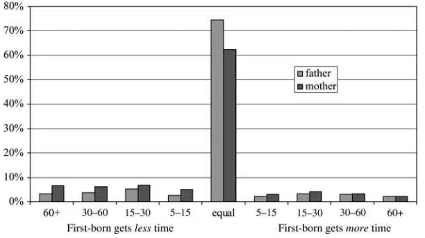
Before describing my empirical strategy, I provide evidence for the two basic facts underlying the explanation for birth-order differences in parent-child time. The first is that parents provide equal time to each child at each point in time. Figure 1 depicts the difference in time allocated on a particular day between the first-and second-born child for all the two-child families in the sample. Figure 1 shows that the majority of parents give equal time to each of their children (74 percent of fathers and 63 percent of mothers). When there is unequal time allocation, it is more likely to favor the younger child, possibly giving the parents the impression that they are actually giving preferential treatment to the second-born child.
The second fact is that parent-child interaction decreases as children age and par-ticularly as the oldest child ages. For example, quality time spent with one’s father drops from 118 minutes each day at age four to 50 minutes at age 13. The corre-sponding drop for quality time with one’s mother is 150 minutes down to 60 minutes.
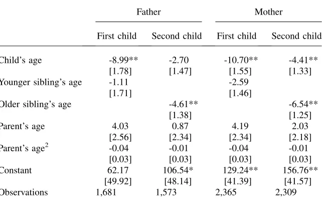
An alternative way to examine this drop in parent-child time as children age is to regress the amount of time received by a child on the child’s age, age of his or her siblings, and other child or family characteristics.6Table 3 provides the results of this
Table 2
Mean Amount of Quality Time Spent with Parent each Day by Age, Family Size, and Birth Order
Father
Family size Birth Order Age 4-5 6-7 8-9 10-11 12-13 Overall
1 1st 89.8 72.7 59.1 54.5 46.8 64.6
2 1st 115.4 96.7 78.4 70.3 47.3 81.6
2nd 92.6 69.0 56.1 50.5 41.9 62.0
3 1st 114.9 76.3 72.7 61.6 81.4
2nd 75.3 72.4 62.0 48.5 64.5
3rd 74.0 55.0 49.4 47.5 56.5
4 1st 101.2 99.3 100.3
2nd 119.3 77.5 98.4
3rd 69.6 65.7 67.7
4th 70.8 46.6 58.7
N 927 1,309 1,410 1,353 1,215 6,214
Mother
Family size Birth Order Age 4-5 6-7 8-9 10-11 12-13 Overall
1 1st 116.0 91.4 80.1 68.8 54.6 82.2
2 1st 177.3 135.8 115.3 92.4 78.4 119.8
2nd 128.5 114.0 84.4 82.0 56.3 93.0
3 1st 167.0 128.9 110.8 82.3 122.3
2nd 131.0 110.0 93.4 63.6 99.5
3rd 107.8 84.1 68.0 64.2 81.0
4 1st 135.0 113.0 124.0
2nd 115.2 110.5 112.8
3rd 118.7 106.6 112.7
4th 99.5 83.3 91.4
N 1,307 1,907 2,068 2,115 1,864 9,261
Note: Each cell in the table is the average quality time spent with a child’s father or mother by the child’s age, family size, and birth order. The ATUS only surveys one adult in each household, so the fathers and mothers in the sample do not come from the same family.
regression separately for the first- and second-born children from two-child families. An interesting result that emerges from this table is that the age of the first-born sib-ling has a much larger effect on the time that both sibsib-lings receive than does the ef-fect of the age of the second-born child. This indicates that the parental time input is determined by the age of the older child and then this time is shared equally with each of the children (possibly due to a sense of fairness).
These two facts are illustrated in this simple diagram:
Figure 1
Each of the solid lines represents a family at a particular point in time with the circles marking the age and time received by the first- and second-born child. These solid lines are horizontal indicating that both children are getting the same amount of parent time even though their ages are different. Comparing the amount of time the two children receive at the same age (the dotted line) reveals the large birth-order gaps in parent-time. The difference in the total time given to the first- and second-born child is the area between the downward-sloping lines drawn through the two sets of plots.
If I had longitudinal time diaries from the same families over a series of years I could simply compare the amount of quality time the first-born child receives at a certain age to the amount of quality time the second-born child receives at the same age. The cross-sectional nature of the data does not allow for this comparison. The strategy of this paper is to compare each child with a child of the same age from a similar family but who has a different birth order. This is done using the nearest neighbor-matching estimator developed by Abadie and Imbens (2002).
I try to get exact matches based on the child’s age, whether the time-diary was for a weekday or weekend, and the education (college graduate, high school graduate, or nei-ther) and labor status (full-time, part-time, or not working) of the parent. In addition, I try to get as close of a match as possible on the parent’s age, marital status (married, cohab-iting, or single), and work status of the parent’s spouse. Using this matching criterion, I obtain the four best matches for each child (more if there are ties) and compare the time
Table 3
Effect of Child’s Age, Sibling’s Age, and Parent’s Age on Quality Time Received (Two-Child Families).
Father Mother
First child Second child First child Second child
Child’s age -8.99** -2.70 -10.70** -4.41**
[1.78] [1.47] [1.55] [1.33]
Younger sibling’s age -1.11 -2.59
[1.71] [1.46]
Older sibling’s age -4.61** -6.54**
[1.38] [1.25]
Parent’s age 4.03 0.87 4.19 2.03
[2.56] [2.34] [2.34] [2.18]
Parent’s age2 -0.04 -0.01 -0.04 -0.01
[0.03] [0.03] [0.03] [0.03]
Constant 62.17 106.54* 129.24** 156.76**
[49.92] [48.14] [41.39] [41.57]
Observations 1,681 1,573 2,365 2,309
received by the first-born child with the amount of time received by the second-born chil-dren to whom he or she is matched. The matching is done with replacement to reduce the bias of the estimate, although it does increase the variance (Abadie and Imbens 2002).
All estimations are run separately by the gender of the parent who responded to the survey and the number of children in the household (each of which can be thought of as other characteristics on which I also have an exact match). While the ATUS is large relative to other time-diary datasets, it is still small relative to the type of data used to employ traditional instruments for family size, such as the gender of the first two children (Angrist and Evans 1998) or the birth of twins (Rosenzweig and Wolpin 1980). As a result, it is difficult to identify a causal link between family size and par-ent-child time. Therefore, I do not examine the impact of family size on parpar-ent-child time, but rather look at birth-order differences within each family size group.
In addition to the matching estimator, I use least squares, tobit, and median regres-sion to estimate birth-order differences in quality time. The tobit estimator corrects for the censored nature of the time children spend with their parents. Of the children in the sample, 11.7 percent of children with mothers responding to the survey spent no quality time with their mother, and 21.6 percent of the children with fathers responding to the survey spent no quality time with their father. Median regression is used as a robustness check to insure that the results are not driven by outliers.
In each of the regressions, I control for the observable characteristics of the parent and child directly, look within family size groups to control for other unobservable parent characteristics, and use indicators of birth order as the variable of interest. The regression takes the following form for families with two, three, or four children:
Tj¼aj+djZ+bj ðbirth orderÞ+ej forj¼2;3;and 4
ð1Þ
whereTis a measure of the amount of quality time the child spent with his or her parent. The vector ‘‘birth order’’ includes indicators for birth order, where the num-ber of included indicators depends on the family size, with the omitted group always being the first-born child. The vectorZis the same set of control variables as in the matching estimator (including the parent’s age, marital status, and work status of spouse). The results of this model are shown for two-, three-, and four-child families in Table 4 along with estimates from the matching estimator.
The results show that for two-child families, the difference in quality time between the first- and second-born child is 22 minutes less with one’s father and 27 minutes less with one’s mother. The difference in three-child families is smaller (16 and 21 minutes) and for four-child families it becomes insignificant. Significant birth-order differences do exist, though, between first- and third- or first- and fourth-born child in the three- and four-child families. The results are also roughly consistent across the different estimation strategies, with slightly smaller estimates for the median regres-sion, as would be expected with the presence of a small set of very large outliers.
The results for the two-child families indicate that the first-born child gets about 37 percent more quality time with his or her father and 28 percent more time with his or her mother than the second-born child.7This translates into a difference of 1,400 hours with one’s father and 1,600 hours with one’s mother across the ages of 4–13.
Father
Two children Three children Four children
Match OLS Tobit Median Match OLS Tobit Median Match OLS Tobit Median
Second child -23.46 -24.39 -21.41 -17.57 -15.59 -18.93 -17.13 -17.13 -7.98 -9.55 -7.09 -18.24 [3.14] [2.25] [2.79] [3.26] [5.03] [3.64] [4.29] [5.14] [14.66] [10.62] [12.12] [9.26]
Third child -28.74 -33.48 -29.69 -27.11 -45.69 -55.07 -47.06 -53.52
[5.75] [5.44] [4.70] [6.06] [15.56] [15.75] [11.86] [10.27]
Fourth child -52.26 -66.71 -49.85 -56.55
[16.92] [19.19] [13.73] [13.15]
N 3,254 1,520 283
(continued)
Price
Table 4 (continued)
Mother
Two children Three children Four children
Match OLS Tobit Median Match OLS Tobit Median Match OLS Tobit Median
Second child -26.24 -29.77 -28.37 -26.31 -22.03 -26.45 -24.43 -21.12 -9.35 -8.80 -9.01 -7.74 [2.80] [2.12] [2.61] [2.91] [4.93] [3.82] [4.17] [5.32] [11.49] [9.18] [10.47] [16.25]
Third child -40.84 -50.47 -45.01 -39.42 -12.37 -9.17 -11.32 -2.36
[5.34] [5.78] [4.69] [6.46] [12.61] [12.58] [12.11] [18.95]
Fourth child -30.93 -30.94 -31.54 -26.10
[15.37] [16.94] [14.33] [24.13]
N 4,674 2,175 429
Note: Standard errors are presented in brackets. The standard errors in the OLS regression are clustered to account for within-family correlation of the error terms. The results in the ‘‘match’’ column come form the nearest neighbor-matching estimator of Abadie and Imbens (2002). The results in the tobit column are the marginal effects following tobit regression and ‘‘median’’ refers to median regression. The dependent variable is the amount of quality time the child spends with his or her parent on the day of the survey. The regressions include controls for type of day, gender of the child, parental age, education, marital status, and work force participation. The bolded elements indicate a significant difference (95 percent level) from the first-born child.
The
Journal
of
Human
One reason that the birth-order differences are smaller in the larger families is that the younger children are excluded from the estimating sample in order to provide enough matches across children of the same age but with a different birth order (chil-dren ages 4-5 are excluded for three-child family analysis and chil(chil-dren ages 4-7 are excluded from the four-child family analysis). Another reason is that the first- and second-born children in larger families tend to be spaced closer in age—an issue ex-plored in the next section.
V. Specification Issues
A. Incomplete Fertility
One concern is that the model only controls for current family size and not the actual family size or the family size that the child will eventually have. The identification strategy depends on being able to compare children from families of the same size with the idea being that children from families of the same size have parents that are similar in the unobservable ways that influence both their family size and time allocation decisions.
The estimates of the effect of birth order in Table 4 will be biased upward if chil-dren in larger families spend more time with their parents.8To make the source of bias more clear, consider two six-year-olds where one has a ten-year-old sibling and the other has a two-year-old sibling. Both have the same current family size but the child with a younger sibling is more likely to be part of a family that will have additional children in the future.
The simplest way to address this issue is to restrict further the age range of the estimation sample. In the extreme case, using just eight- and nine-year-old children from two child families reduces dramatically the chances of there being additional children who have either left home or are not born yet. Table 5 provides estimates of birth-order differences using the OLS regression approach for a wide set of age ranges. The rows indicate the lower bound of the age range (ages 4-8) and the col-umns indicate the upper bound of the age range (ages 8–13). Rather than present the coefficients and standard errors for each estimation (as in Table 4), I provide the per-centage difference between the first- and second-born children. This number is cal-culated by dividing the point estimate for the group by the average for the children used in the estimation.
The results in Table 5 show that the birth-order difference is robust to this wide set of age ranges and persists even when looking at a very narrow age range for which the chances that current family size differs from actual or eventual family size is very small. For mothers, there is very little variation across the cells and no discernible pattern. For fathers, the variation across cells is a little higher with some suggestive evidence that the birth-order difference (in percentage terms) is larger when restrict-ing the sample to the younger age groups.
B. Sibling Characteristics
A second issue is whether birth-order differences vary based on important sibling characteristics such as gender composition and birth spacing. I address this issue us-ing the subset of families with two children. This group provides a parsimonious way of constructing measures for gender composition and birth spacing that would be-come overly complex if applied to larger families.
The effect of gender composition of siblings on birth-order differences is esti-mated by interacting the gender of the two children with the birth order of the indi-vidual child:
Table 5
Birth Order Differences for Alternative Age Ranges in Terms of Percentage Differences (Two-child Families)
Father
Upper-bound
Lower-bound 8 9 10 11 12 13
4 34.6% 32.7% 32.9% 34.3% 32.1% 31.6%
5 36.6% 33.8% 33.6% 35.1% 32.4% 31.9%
6 39.9% 35.1% 34.6% 36.0% 32.7% 31.9%
7 31.0% 26.7% 28.1% 31.0% 27.8% 27.2%
8 33.8% 24.8% 27.4% 31.3% 27.1% 26.4%
Mother
Upper-bound
Lower-bound 8 9 10 11 12 13
4 27.3% 29.0% 28.7% 27.6% 28.4% 29.0%
5 25.5% 27.8% 27.4% 26.2% 27.2% 28.0%
6 25.1% 27.9% 27.2% 25.7% 26.9% 27.7%
7 29.0% 31.8% 29.8% 27.4% 28.7% 29.4%
8 24.0% 30.8% 27.8% 25.1% 27.2% 28.2%
Ti¼ +
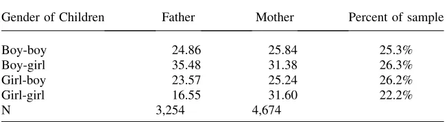
The omitted group in this estimation is the first-born child in a boy-boy family. Table 6 provides the difference in predicted values between the first- and second-born child of each sex composition group. The far right column in Table 6 shows the fraction of two-child families in my sample that fall into each sex composition group. The results in Table 6 show that the birth-order differences in time spent with one’s father are greatest when the first child is a boy and the second child is a girl. This result supports the type of paternal preference for sons found by Dahl and Moretti (2005). Table 7 provides results of a similar analysis except that the birth order of the child is interacted with the difference in age between the two siblings:
Ti¼ +
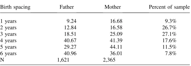
The first-born children from families with a birth spacing of three years serve as the omitted group. Using the estimated coefficients from the equation, I calculate the dif-ference in predicted values between the amount of time received by the first- and sec-ond-born child for each of the birth spacing groups. These differences are reported in Table 7. These results show that there is a general pattern in which birth-order differ-ences increase with birth spacing, with relatively small birth-order differdiffer-ences when the children are spaced one or two years apart.
C. Alternative Measures of Parent-child Interaction
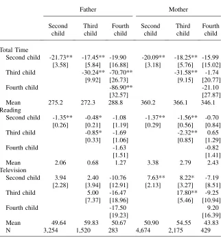
A final issue relates to how sensitive the birth-order differences are to the particular measure of parent-child interaction. Up to this point, the measure of quality time includes the 13 activities listed in the upper panel of Appendix Table A1. In Table 8, I examine three alternative measures of parent-child interaction: total time spent
Table 6
Birth Order Differences in Quality Time by Sibling Gender Composition (Two child Families, Children Ages 4–13)
Gender of Children Father Mother Percent of sample
Boy-boy 24.86 25.84 25.3%
Boy-girl 35.48 31.38 26.3%
Girl-boy 23.57 25.24 26.2%
Girl-girl 16.55 31.60 22.2%
N 3,254 4,674
together, time spent reading, and time spent watching television together. Total time includes the amount of time that a child is present (in the same room, car, etc) as his or her parent and makes no distinction as to what the parent was doing as the time. Reading together is generally thought to be of the greatest importance in child’s de-velopment and performance in school. Time spent watching television and movies together are included as a measure of noninteractive time that is generally thought to have a negative impact on child outcomes or at least crowd out better activities.9 The results in Table 8 show that in two child families, the second child gets 10 per-cent less total time, 41 perper-cent less time reading, and 15 perper-cent more time watching television with his or her mother. The corresponding differences for time with one’s father are 14 percent less total time, 66 percent less reading time, and 8 percent more time watching television.10These results provide one explanation for the birth-order differences in quality time. The second-born child gets slightly less total time with their parent and of the time they do receive, quality time is being crowded out by other activities, such as watching television.
Appendix Table A2 provides results using various cutoffs in the spectrum of parent-child activities in Appendix Table A1. In terms of percentage differences, the largest birth-order differences occur when restricting the quality time measure to the six ac-tivities that are thought to have the most significant impact on the human capital of
Table 7
Birth Order Differences in Quality Time by Birth Spacing (Two child Families, Children Ages 7–11)
Birth spacing Father Mother Percent of sample
1 years 9.24 16.68 9.3%
2 years 12.84 16.58 26.7%
3 years 18.51 25.09 27.1%
4 years 40.67 41.39 17.6%
5 years 29.27 44.11 11.5%
6 years 40.96 36.01 7.8%
N 1,621 2,365
Note: Each element is the birth order difference between first- and second-born children in two-child fam-ilies based on the difference in predicted values following an OLS regression which includes the same set of covariates as Table 3 but with the birth-order indicator replaced with the interaction of birth order and the birth spacing of the two children. Differences significant at 5 percent level are bolded.
9. Gentzho and Shapiro (2006), however, provide some evidence that the introduction of television in the 1960s had no major negative consequences for children’s cognitive outcomes. The general consensus among pediatricians is that television usage should be limited to no more than one or two hours a day (American Academy of Pediatricians 2001).
the child: reading, playing, helping with homework, talking, teaching, and doing arts and crafts together (Bianchi and Robinson 1997, Zick et al. 2001).
VI. Aggregate Birth-order Differences
The birth-order differences calculated up to this point have controlled for the parent’s age. One difference between a first- and second-born child is the age
Table 8
Birth Order Differences Using Alternative Measures of Parent-child Time
Father Mother
Second child -21.73** -17.45** -19.90 -20.09** -18.25** -15.99
[3.58] [5.84] [16.88] [3.18] [5.76] [15.02]
Third child -30.24** -70.70** -31.58** -1.74
[9.92] [26.73] [9.15] [20.77]
Fourth child -86.90** -21.10
[32.57] [27.87]
Mean 275.2 272.3 288.8 360.2 366.1 346.1
Reading
Second child -1.35** -0.48* -1.08 -1.37** -1.56** -0.70
[0.26] [0.21] [1.19] [0.29] [0.56] [0.84]
Third child -0.85* -1.69 -2.32** 0.65
[0.33] [1.06] [0.85] [1.29]
Fourth child -1.63 -0.82
[1.51] [1.41]
Mean 2.06 0.68 1.27 3.38 2.79 2.43
Television
Second child 3.94 2.40 -10.76 7.63** 8.22* -7.19
[2.28] [3.94] [12.91] [2.13] [3.27] [8.51]
Third child 5.00 -16.47 17.80** -9.25
[7.37] [18.96] [5.46] [10.94]
Fourth child -17.50 9.20
[19.23] [16.39]
Mean 49.64 59.83 50.67 50.90 54.55 43.83
N 3,254 1,520 283 4,674 2,175 429
of their parents when the child reaches a given age. The estimations also only have examined the amount of time a child spends with a particular parent with no distinc-tion made between when one or both parents are present. This final secdistinc-tion addresses these issues by calculating the net effect of a child’s birth order using a simulation of the amount of parent-child interaction across ages four through thirteen. The results provide an idea of the magnitude of the birth-order difference in quality time over an important period of the child’s life.
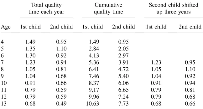
The sample used in the simulation is restricted to families with two children. This makes it possible to interact birth order with the child’s age, creating a set of 20 in-dicator variables (two birth-order groups and ten age groups). In addition, I interact each of the parent characteristics with the age groups. Table 9 contains the simulated amount of time that each child spends with his or her parents at each age. The specific case examined in the table is a two-child family where the parents are married, college-educated, and both work full-time. Both parents were 29 when the first child was born and they have two boys spaced three years apart. The parent age at first birth, marital status, and work status all represent the modal group of the data.
The third and fourth columns of Table 9 show the cumulative time that a child spends with his parents. Between the ages of 4 and 13, the first-born child spends
Table 9
Simulated Amount of Quality Time Spent with Parents at Each Age (in 1,000Õs of hours/year)
Total quality time each year
Cumulative quality time
Second child shifted up three years
Age 1st child 2nd child 1st child 2nd child 1st child 2nd child
4 1.49 0.95 1.49 0.95
5 1.35 1.10 2.84 2.05
6 1.30 0.92 4.13 2.97
7 1.23 0.94 5.36 3.91 1.23 0.95
8 1.05 0.81 6.41 4.72 1.05 1.10
9 1.04 0.68 7.46 5.40 1.04 0.92
10 0.91 0.66 8.37 6.06 0.91 0.94
11 0.79 0.59 9.17 6.65 0.79 0.81
12 0.79 0.59 9.96 7.24 0.79 0.68
13 0.68 0.49 10.63 7.73 0.68 0.66
10,630 hours in quality time with his or her parents and the second-born child spends about 7,730 hours. The difference of 2,900 hours represents about a 38 percent in-crease over the time that second child receives and translates into a difference of 48 minutes each day.
The simulation in Table 9 combines both father time and mother time. This leads to a double counting of all time in which both parents were present. Past research usually asserts that parents try to maximize the amount of time that at least one of them is with the children, but no research has addressed the relative value of spend-ing time with one parent compared two parents in terms of development. Folbre et al. (2005) note that when both parents are present there is less stress on the adults and the children get to see their parents interacting with each other.
An alternative measure is the amount of quality time the child receives with at least one parent present (thus setting the benefit of the additional parent’s presence to zero). The first-born children in the sample receive 47 minutes of quality time each day with both parents present. The amount for second-born children is 36 minutes. This aggregates across ages 4–13 into 2,860 hours for the first child and 2,190 hours for the second child. Subtracting these from the simulation results shows that the first child receives 7,770 hours of quality time with at least one parent present while the second child receives 5,540 hours. This leads to a birth-order difference of 2,230 hours, which is a 40 percent difference and translates into about 37 minutes each day. The last two columns of Table 9 provide the same cumulative measures as the middle two columns but with the second child’s time shifted forward three years to make it easier to compare the amount of quality time they receive the same point in time. The last two columns show that in each year the time allocation to each child is roughly equal (matching the results in Figure 1 described earlier).
VII. Conclusion
The primary contribution of this paper is that it provides clear evi-dence of large birth-order differences in the amount of quality time that children spend with their parents. A first-born child in a two-child family spends about 20– 25 more minutes each day engaging in quality-time activities with his or her father than the second-born child. The difference in quality time with one’s mother for the same group is about 25–30 minutes. Birth-order differences also exist when com-paring second- and third-born children or other birth-order combinations in larger families.
Of course, potentially offsetting effects may favor second-born children. One pos-sibility is that parents may become more efficient at certain tasks such that less time is needed to provide the same amount of care. This is certainly true for physical-care activities, such as changing diapers or dressing children. However, the birth-order differences are largest in the specific activities, which are thought to have the greatest impact on a child’s human capital (such as reading and playing) and for which it is much less likely that parents experience efficiency gains.
Another possible offsetting effect is that younger siblings may benefit from the in-put of older siblings and hence require less time with parents. However, the sibling benefits go in both directions. Zajonc (1976) asserts (as one of the main assumptions of the confluence model) that older siblings benefit more by teaching younger sib-lings than the younger sibsib-lings benefit from being taught. It is also not hard to imag-ine that many of the things that children learn from their older siblings may actually have a negative impact.
The second contribution of this paper is that it provides an alternative view as to how parents allocate resources to their children. The model of Becker and Tomes (1976) hypothesizes that parents will invest their time in the more able child (while equalizing lifetime outcomes by transferring more wealth to the less able child). The results of this paper show rather that parents divide their time resources equally among their children at each point in time.11However, inter-temporal inequities arise because the amount of parent-child interaction that occurs is decreasing as the chil-dren age such that the second child receives less time at each age than the first-born did at the same age. This provides an interesting case where the desire to provide equal treatment actually creates inequality.12
A third contribution of this paper is that it provides motivation to include birth spacing in the analysis of birth order and child outcomes. Given that family resources generally increase with time, larger birth spacing will create a greater difference in the financial resources available by birth order, favoring the younger child (Behrman and Taubman 1986, Powell and Steelman 1995). The results in this paper show that the opposite will be true in terms of time resources. This could allow future work to exploit these opposing forces to test the relative contribution of time and money to child outcomes.
11. This result of equal time allocation matches the results of Menchik (1979), Wilhelm (1996), and McGarry (1999), which show that the majority of bequests involve equal division among children. Light and McGarry (2004) explore the reasons that unequal bequests occur.
Fraction
Activity description
Fraction of children with
time>0
Mean of those with time>0
Total time across sample
Mean across sample
Alone Time (second child)
Alternate categories
Included in quality time
Reading to/with 8.0% 31.5 31,012 2.51 23.2% A
Playing, not sports 11.4% 97.1 136,162 11.04 9.5% A
Helping with homework 11.1% 57.9 79,036 6.41 26.2% A
Talking with/listening 9.3% 33.6 38,410 3.11 21.1% A
Helping/teaching 1.6% 39.2 7,641 0.62 32.2% A
Arts and crafts with 0.3% 42.7 1,750 0.14 29.9% A
Eating together 73.7% 56.4 513,009 41.59 5.9% B
Playing sports with 1.4% 72.5 12,829 1.04 21.5% C
Attending performing arts 0.5% 106.7 5,973 0.48 19.8% C
Attending museums 0.3% 174.3 6,099 0.49 5.8% C
Participating in religious practices 1.6% 25.0 5,005 0.41 4.2% C
Looking after (as primary activity) 7.5% 70.6 65,513 5.31 9.8% D
Physical care for 47.5% 48.9 286,151 23.20 11.4% D
(continued)
Price
Table A1 (continued)
Fraction
Activity description
Fraction of children with
time>0
Mean of those with time>0
Total time across sample
Mean across sample
Alone Time (second child)
Alternate categories
Not included in quality time
Organizing and planning for 2.3% 21.0 5,913 0.48 19.3% E
Attending events 3.8% 110.3 52,184 4.23 25.9% E
Picking up/dropping off 21.8% 11.7 31,560 2.56 27.6% E
Meetings and school conferences 0.5% 47.7 3,005 0.24 35.1% E
Traveling together 41.9% 56.0 289,640 23.48 16.7% E
Watching television 39.5% 131.7 642,172 52.06 13.8% —
Note: The unit of analysis above is the individual child, but each measure refers to the amount of time the child spent engaged in the activity with their parent. ‘‘Fraction alone time’’ is the fraction of parent-child time in which no other siblings were present (using sub-sample of families with only two children). The main quality time measure used throughout the paper includes Categories A–D. Appendix Table A2 provides results using a range of different cutoffs for quality time. Sample size is 12,335 and includes all children ages 4–13 from families with 2–4 children.
The
Journal
of
Human
References
Abadie, Alberto, and Guido Imbens. 2002. ‘‘Simple and Bias-Corrected Matching Estimators for Average Treatment Effects.’’ National Bureau of Economic Research Technical Working Paper no. 283.
Aizer, Anna. 2004. ‘‘Home Alone: Supervision After School and Child Behavior.’’Journal of
Public Economics88(9):1835–48.
Amato, Paul, and Fernando Rivera. 1999. ‘‘Paternal Involvement and Children’s Behavior
Problems.’’Journal of Marriage and the Family61(2):375–84.
Table A2
Birth Order Differences Using Alternative Measures of Quality Time
Father Mother
Second child -9.75** -9.14** -3.56 -8.49** -8.65** -1.97
[1.37] [2.44] [5.38] [1.28] [2.23] [5.80]
Third child -15.25** -24.99** -16.60** -3.00
[3.63] [9.32] [3.34] [8.41]
Fourth child -21.42 -8.24
[11.53] [10.72]
Mean 18.29 18.80 28.19 29.42 26.51 29.17
Type A–C activities
Second child -13.78** -9.92** -2.32 -12.53** -11.60** -3.96
[1.88] [3.23] [8.32] [1.66] [2.97] [6.97]
Third child -16.08** -46.12** -23.56** -2.13
[4.88] [12.95] [4.51] [10.46]
Fourth child -46.67** -8.57
[16.03] [13.91]
Mean 55.05 51.70 67.74 69.54 65.42 68.57
Type A–E activities
Second child -25.68** -19.85** -9.14 -27.72** -26.46** -8.80
[2.83] [4.35] [12.85] [2.49] [4.72] [12.10]
Third child -35.24** -54.24** -49.37** 7.51
[6.76] [17.73] [7.36] [17.43]
Fourth child -69.41** -30.30
[21.32] [22.16]
Mean 95.85 86.68 103.35 138.64 136.93 145.76
N 3,254 1,520 283 4,674 2,175 429
American Academy of Pediatricians. 2001. ‘‘Children, Adolescents, and Television.’’ Pediatrics107(2):423–26.
Angrist, Joshua, and William Evans. 1998. ‘‘Children and Their Parents’ Labor Supply:
Evidence from Exogenous Variation in Family Size.’’American Economic Review
88(3):450–77.
Argys, Laura; Daniel Rees, Susan Averett, and Benjamin Witoonchart. 2006. ‘‘Birth Order
and Risky Adolescent Behavior.’’Economic Inquiry44(2):215–33.
Becker, Gary, and Nigel Tomes. 1976. ‘‘Child Endowments and the Quantity and Quality of
Children.’’Journal of Political Economy84(4):S143–62.
Behrman, Jere. 1997. ‘‘Intrahousehold Distribution and the Family.’’Handbook of Population
Economics, ed. Mark Rosenzweig and Oded Stark, 125–87. Amsterdam: North-Holland. Behrman, Jere, Robert Pollak, and Paul Taubman. 1982. ‘‘Parental Preferences and Provision
for Progeny.’’The Journal of Political Economy90(1):52–73.
Behrman, Jere, and Paul Taubman. 1986. ‘‘Birth Order, Schooling, and Earnings.’’Journal of
Labor Economics4(3):S121–145.
Bianchi, Suzanne, and John Robinson. 1997. ‘‘What Did You Do Today? Children’s Use of
Time, Family Composition, and the Acquisition of Social Capital.’’Journal of Marriage
and the Family59(2):332–44.
Black, Sandra, Paul Devereux, and Kjell Salvanes. 2005. ‘‘The More the Merrier? The Effect
of Family Size and Birth Order on Children’s Education.’’Quarterly Journal of Economics
120(2):669–700.
Blake, Judith. 1989.Family Size and Achievement.Berkeley and Los Angeles, Calif.:
University of California Press.
Blau, Francine, and Adam Grossberg. 1992. ‘‘Maternal Labor Supply and Children’s
Cognitive Development.’’The Review of Economics and Statistics74(3):474–81.
Booth, Allison, and Hiau Joo Kee. 2006. ‘‘Birth Order Matters: The Effect of Family Size and Birth Order on Educational Attainment.’’ Centre for Economic Policy Research Discussion Paper no. 5453.
Cabrera, Natasha, Catherine Tamis-LeMonda, Robert Bradley, Sandra Hofferth, and Michael
Lamb. 2000. ‘‘Fatherhood in the Twenty-First Century.’’Child Development71(1):127–36.
Conley, Dalton, and Rebecca Glauber. 2006. ‘‘Parental Education Investment and Children’s Academic Risk: Estimates of the Impact of Sibship Size and Birth Order from Exogenous
Variation in Fertility.’’Journal of Human Resources41(4):722–37.
Dahl, Gordon, and Enrico Moretti. 2004. ‘‘The Demand for Sons: Evidence from Divorce, Fertility, and Shotgun Marriage.’’ National Bureau of Economic Research Working Paper no. 10281.
Datcher-Loury, Linda. 1988. ‘‘Effect of Mother’s Home Time on Children’s Schooling.’’ Review of Economics and Statistics70(3):367–73.
Eisenberg, Marla, Rachel Olson, Dianne Neumark-Sztainer, Mary Story, and Linda Bearinger. 2004. ‘‘Correlations Between Family Meals and Psychosocial Well-being Among
Adolescents.’’Pediatrics and Adolescent Medicine158(8):792–96.
Folbre, Nancy, Jayoung Yoon, Kade Finnoff, and Allison Sidle Fuligni. 2005. ‘‘By What
Measure? Family Time Devoted to Children in the United States.Demography
42(2):373–90.
Gary-Bobo, Robert; Ana Prieto, and Nathalie Picard. 2006. ‘‘Birth-Order and Sibship Sex-Composition Effects in the Study of Education and Earnings.’’ Centre for Economic Policy Research Discussion Paper no. 5514.
Gerner, Jennifer, and Dean Lillard. 2006. ‘‘The Effect of Birth Order on Early Educational Attainment.’’ Cornell University. Unpublished.
Hamermesh, Daniel, Harley Frazis, and Jay Stewart. 2005. ‘‘Data Watch: The American Time
Use Survey.’’Journal of Economic Perspectives19(1):221–32.
Hanushek, Eric. 1992. ‘‘The Trade-off Between Child Quantity and Quality.’’Journal of
Political Economy100(1):84–117.
Hauser, Robert, and William Sewell. 1985. ‘‘Birth Order and Educational Attainment in Full
Sibships.’’American Educational Research Journal22(1):1–23.
Hertwig, Ralph, Jennifer Nerissa Davis, and Frank Sulloway. 2002. ‘‘Parental Investment:
How an Equity Motive Can Produce Inequality.’’Psychological Bulletin128(5):728–45.
Hill, M. Anne, and June O’Neill. 1994. ‘‘Family Endowments and the Achievement of Young
Children with Special Reference to the Underclass.’’Journal of Human Resources
29(4):1064–1100.
Iacovou, Maria. 2001. ‘‘Family Composition and Children’s Educational Outcomes’’ Institute for Social and Economic Research Working paper 2001–12.
Kessler, Daniel. 1991. ‘‘Birth Order, Family Size, and Achievement: Family Structure and
Wage Determination.’’Journal of Labor Economics9(4):413–26.
Leibowitz, Arleen. 1977. ‘‘Parental Inputs and Children’s Achievement.’’The Journal of
Human Resources12(2):242–51.
Light, Audrey and Kathleen McGarry. 2004. ‘‘Why Parents Play Favorites: Explanations for
Unequal Bequests.’’American Economic Review94(5):1669–81.
Lindert, Peter. 1977. ‘‘Sibling Position and Achievement.’’Journal of Human Resources
12(2):198–219.
McGarry, Kathleen. 1999. ‘‘Inter Vivos Transfers and Intended Bequests.’’Journal of Public
Economics73(3):321–51.
Menchik, Paul. 1979. ‘‘Inter-generational Transmission of Inequality: An Empirical Study of
Wealth Mobility.’’Economica46(184):349–62.
Pleck, Joseph. 1997. ‘‘Paternal Involvement: Levels, Origins, and Consequences.’’ InThe
Role of the Father in Child Development, 3rd ed., ed.Michael Lamb, 66–103. New York: Wiley.
Powell, Brian, and Lala Carr Steelman. 1995. ‘‘Feeling the Pinch: Child Spacing and
Constraints on Parental Economic Investments in Children.’’Social Forces73(4):1465–86.
Rosenzweig, Mark, and Kenneth Wolpin. 1980. ‘‘Testing the Quantity-Quality Fertility
Model: The Use of Twins as a Natural Experiment.’’Econometrica48(1):227–40.
Se´ne´chal, Monique, and Jo-Anne LeFevre. 2002. ‘‘Parental Involvement in the Development
of Children’s Reading Skill: A Five-Year Longitudinal Study.’’Child Development
73(2):445–60.
Snow, Catherine, M. Susan Burns, and Peg Griffin. 1998.Preventing Reading Difficulties in
Young Children.Washington, D.C.: National Academy Press.
Steelman, Lala; Brian Powell, Regina Werum, and Scott Carter. 2002. ‘‘Reconsidering the
Effects of Sibling Configuration: Recent Advances and Challenges.’’Annual Review of
Sociology28(1):243–69.
Taveras, Elsie, Sheryl Rifas-Shiman, Catherine Berkey, Helaine Rockett, Alison Field, A. Lindsay Frazier, Graham Colditz, and Matthe Gillman. 2005. ‘‘Family Dinner and
Adolescent Overweight.’’Obesity Research13(5):900–906.
Wilhelm, Mark. 1996. ‘‘Bequest Behavior and the Effect of Heirs’ Earnings: Testing the
Altruistic Model of Bequests.’’American Economic Review86(4):874–92.
Zajonc, Robert. 1976. ‘‘Family Configuration and Intelligence.’’Science192(4236):227–36.
Zick, Cathleen, W. Keith Bryant, and Eva O¨ sterbacka. 2001. ‘‘Mother’s Employment,
Parental Involvement, and the Implications for Children’s Behavior.’’Social Science