This ar t icle was dow nloaded by: [ Univer sit as Dian Nuswant or o] , [ Rir ih Dian Prat iw i SE Msi] On: 29 Sept em ber 2013, At : 19: 20
Publisher : Rout ledge
I nfor m a Lt d Regist er ed in England and Wales Regist er ed Num ber : 1072954 Regist er ed office: Mor t im er House, 37- 41 Mor t im er St r eet , London W1T 3JH, UK
Accounting and Business Research
Publ icat ion det ail s, incl uding inst ruct ions f or aut hors and subscript ion inf ormat ion:
ht t p: / / www. t andf onl ine. com/ l oi/ rabr20
Bounded variation and the asymmetric
distribution of scaled earnings
Demet ris Christ odoul ou a & St uart McLeay b a
MEAFA, Facul t y of Economics and Business, The Universit y of Sydney, NSW, 2006, Aust ral ia E-mail :
b
Universit y of Sussex
Publ ished onl ine: 04 Jan 2011.
To cite this article: Demet ris Christ odoul ou & St uart McLeay (2009) Bounded variat ion and t he asymmet ric dist ribut ion of scal ed earnings, Account ing and Business Research, 39: 4, 347-372, DOI: 10. 1080/ 00014788. 2009. 9663372
To link to this article: ht t p: / / dx. doi. org/ 10. 1080/ 00014788. 2009. 9663372
PLEASE SCROLL DOWN FOR ARTI CLE
Taylor & Francis m akes ever y effor t t o ensur e t he accuracy of all t he infor m at ion ( t he “ Cont ent ” ) cont ained in t he publicat ions on our plat for m . How ever, Taylor & Francis, our agent s, and our licensor s m ake no r epr esent at ions or war rant ies w hat soever as t o t he accuracy, com plet eness, or suit abilit y for any pur pose of t he Cont ent . Any opinions and view s expr essed in t his publicat ion ar e t he opinions and view s of t he aut hor s, and ar e not t he view s of or endor sed by Taylor & Francis. The accuracy of t he Cont ent should not be r elied upon and should be independent ly ver ified w it h pr im ar y sour ces of infor m at ion. Taylor and Francis shall not be liable for any losses, act ions, claim s, pr oceedings, dem ands, cost s, expenses, dam ages, and ot her liabilit ies w hat soever or how soever caused ar ising dir ect ly or indir ect ly in connect ion w it h, in r elat ion t o or ar ising out of t he use of t he Cont ent .
Bounded variation and the asymmetric
distribution of scaled earnings
Demetris Christodoulou and Stuart McLeay
*Abstract—This paper proposes afinite limits distribution for scaled accounting earnings. The probability density function of earnings has been the subject of a great deal of attention, indicating an apparent‘observational discontinuity’at zero. Paradoxically, the customary research design used in such studies is built on the implied assumption that the distribution of scaled accounting earnings should approximate a continuous normal variable at the population level. This paper shows that such assumptions may be unfounded, and, using large samples from both the US and the EU, the study provides alternative evidence of a consistently asymmetric frequency of profits and losses. This casts further doubt on the interpretation of the observed discontinuity in the distribution of earnings as prima facie evidence of earnings management. A particular innovation in this paper is to scale the earnings variable by the magnitude of its own components, restricting the standardised range to [–1,1]. Nonparametric descriptions are provided that improve upon the simple histogram, together with non-normal parametric probability estimates that are consistent with the scalar that is proposed. A notable advantage of this approach is that it avoids some of the statistical shortcomings of commonly used scalars, such as influential outliers and infinite variances.
Keywords: accounting earnings; scalars; deflators; boundary conditions; parametric and nonparametric density estimation
1. Introduction
The probability density function of accounting earnings has attracted a great deal of attention, especially in understanding the distribution of earnings in different settings (e.g. Dechow et al., 2003; Burgstahler and Eames, 2003; Leuz et al., 2003; Brown and Caylor, 2005; Peasnell et al., 2005; Yoon, 2005; Daske et al., 2006; Maijoor and Vanstraelen, 2006; Gore et al., 2007). However, a problematic feature of research design in this area is that the use of an earnings deflator may introduce sample bias. Indeed, according to Durtschi and Easton (2005), the observed discontinuity in the distribution of earnings could be a spurious result that is due to scaling by variables that are system-atically lower for loss observations than for profit observations. But other researchers (Beaver et al., 2007; Jacob and Jorgensen, 2007; Kerstein and Rai, 2007) have since rejected the arguments put forward by Durtschi and Easton, and claim that the abrupt changes documented at zero earnings are
not primarily attributable to scaling.1Whilst there is a growing body of work that already questions the assertion that the observed discontinuity is simply a statistical effect, it is noticeable nevertheless that earnings management studies are now being designed with alternative scalars in mind (e.g. Petrovits, 2006; Daniel et al., 2008).
In this paper, we consider another shortcoming that may lead researchers to question the conclu-sions arrived at regarding the distribution of earn-ings, and in this context we propose an entirely new scalar with some remarkable properties. In essence, our main concern is that inferences about scaled accounting earnings are generally drawn by pre-suming normality in the limit. This gives rise to an obvious contradiction in research design when the
*The authors are at the University of Sydney and the University of Sussex. They are grateful for the helpful contributions of Maurice Peat, Maxwell Stevenson and Jo Wells. They also thank the anonymous reviewers for construct-ive comments.
Further details of the authors’statistical programming code are available at http://meafa.econ.usyd.edu.au/.
Correspondence should be addressed to: Dr Demetris Christodoulou, MEAFA, Faculty of Economics and Business, The University of Sydney, NSW 2006, Australia. E-mail: d.christodoulou@econ.usyd.edu.au.
This paper was accepted for publication in February 2009. 1
Durtschi and Easton (2005) suggest scaling by the number of shares, and the visual evidence published by these authors suggests that, for earnings per share, the distribution is smoother around zero than was previously documented using other scalars. However, Beaver, et al. (2007) are at odds with this view, and their evidence reveals that the number of outstanding shares tends, in practice, to be higher for losses than profits, which has the effect of shifting scaled loss observations towards zero, and could therefore be responsible for the reduction in the kink in the distribution of earnings when scaled by the number of shares. Jacob and Jorgensen (2007) and Kerstein and Rai (2007) also reject the arguments put forward by Durtschi and Easton, documenting abrupt changes at zero that are not primarily attributable to scaling. The impact of this recent research is now evident in additional testing for such biases– see for example Ballantine et al. (2007) who use a lagged total assets scalar in examining earnings management in hospital trusts, and test accordingly for any systematic difference in the size of the scalar across surplus and deficit trusts.
apparent ‘discontinuity’ about zero earnings is evaluated in an asymptotic Gaussian setting with a (supposedly) random sampling offirms. In theory, such a design implies that, as the sample size tends towards its population limit, the less the observed
‘discontinuity’ would be and that eventually it would vanish. If, however, a disproportion is expected around zero regardless of sample size, then expectations should not be based on the normal curve and an alternative framework is required, using either a suitable nonparametric approach or a more appropriate parametric model. This paper introduces such a framework, together with the appropriate scalar.
To illustrate, Figure 1 provides a histogram of the central empirical frequencies of net income scaled by sales, using the sample that is employed in this research study. The lack offit to the normal curve that can be seen around zero is generally interpreted as prima facie evidence of earnings management, but, as mentioned already, this inference depends on the appropriateness of the normality assumption for the population.2Figure 1 also clearly demonstrates how inferences concerning the conjectured discon-tinuity depend on the origin and bin width of the histogram estimator. In this respect, it is usual to examine the difference between the observed probability of earnings for the ithbin next to zero (estimated aspi¼ni=n, wherenis the total number of observations andnithe number of observations that fall in theithbin) and an expected probability that is calculated as the average of the two adjacent bins, i.e.E pð Þ ¼i ðpi 1þpiþ1Þ=2. If the normalised difference jpi E pð Þji =std:error is large, then the observational disproportion around zero is taken as an indication of earnings management. However, the histogram itself defines the weight of the observed probabilitiespi, and Figure 1 shows how a bin width and origin that are selected to separate the groupings at zero will bias the nonparametric representation in a way that emphasises this disproportion.3
In view of the implicit shortcomings outlined
above, and in the light of the debate initiated by Durtschi and Easton (2005), we motivate this paper by first explaining why we might expect an asymmetric shape in net income, not simply as the outcome of earnings management but for more fundamental reasons. Then we describe an approach to modelling earnings using a scalar which reflects the magnitude of the components of income, from which we derive a measure of scaled accounting earnings with known bounds. A major benefit of the known range of variation under the transformation is that the distributional space remains standardised for all observations regardless of the sample size and the degree of heterogeneity. Indeed, we are able to show how the variation of scaled accounting earnings asymptotically approxi-mates the limits that are reached in the extreme cases where firms report either zero costs or zero sales. To examine the shape of the earnings distribution, a kernel density estimator is employed that provides a more detailed and unbiased descrip-tion than the commonly-used histogram estimator, showing that net income is consistently asymmetric across samples drawn from different economic regions and different accounting jurisdictions. The paper also derives a bounded parametric density function with the ability to accommodate such asymmetry, which is analytically superior to the standard normal. Given the above, we conclude with evidence that the key characteristic of scaled accounting earnings is its asymmetry, and it is suggested in the final discussion that this may be attributable to a great extent to firm-level hetero-geneity effects, as the asymmetry is removed when we examine mean-adjusted densities at the firm level.
2. The distribution of accounting earnings
In this paper, we argue that normality in scaled earnings is not consistent with the character of the accounting variables involved in calculating and2This type of analysis dates back to Burgstahler and Dichev (1997) and Degeorge et al. (1999), who investigate bottom-line net income, as we do in this paper. They scale net income by market value and number of shares respectively. For a sample of firm-year earnings, they each observe a disproportionate frequency around zero and attribute this result to the upwards management of earnings, in the sense that listedfirms with small losses attempt to beat the benchmark of zero and thus report small profits. Degeorge et al. (1999) test the null hypothesis that the density of earnings is smooth at the point of interest, assuming that the change in probability from binito bini+1 is approximately normal. We infer that this implies normality in the parent distribution as the sum of normal variates is itself normal.
3
It is a common practice to round the number of bins to the nearest even integer and then to compute the expected valueE
(pi), so that the bins are separated at zero. Figure 1 illustrates the
potential misrepresentation that is inherent in this approach by comparing two histograms with the same origin and range, with one separating at zero and the other having an odd number of bins and therefore not separating at zero. A histogram with 30 bins generates the well-documented difference in probabilities around zero, withpi–E(pi) in the negative bin adjacent to zero
equal to 0.0497 for the EU and 0.0305 for the US, the difference in the positive bin adjacent to zero being equal to 0.0467 for the EU and 0.0325 for the US. However, when we estimate a histogram with 29 bins, we find little difference between the observed and expected probabilities for the bin which contains the point zero (–0.0097 for the EU and 0.0007 for the US), and what is more, the shape no longer implies an observational disproportion at zero.
348 ACCOUNTING AND BUSINESS RESEARCH
scaling earnings. To start with, the double-entry bookkeeping system that generates earnings requires a one-to-one correspondence between debits and credits that cannot be related to the
randomness of normal probability laws (Ellerman, 1985; Cooke and Tippett, 2000). Indeed, the seminal work of Willett (1991) on the stochastic nature of accounting calculations provides a general
Figure 1
The frequency distribution of net income scaled by sales
Note:The histograms describe the frequencies of net income scaled by sales within the range [–0.25, 0.25],
for 48,563 EUfirm-years and 104,170 USfirm-years covering the period 1985–2004. The shaded histogram
has 29 bins and the histogram drawn in outline has 30 bins. In the latter case, bin separation at zero conveys the impression of a‘discontinuity’at zero, whereas the empirical frequencies depicted by the shaded histogram appear much smoother. For each plot, the superimposed dashed curve represents the normal curvefitted with the mean and standard deviation of the sample, displayed here over the range [–0.25,0.25].
proof that bookkeeping figures, and earnings in particular, may be better represented as determinis-tic measures of random variables. Given that double-entry bookkeeping is a series of algebraic operations on ordered pairs of such numbers, it is evident that the accounting process creates an endogenous matrix of linearly related information, which will include all of the components of earnings and each of the book-based scalars commonly used in accounting research. These relationships will in turn determine the variance of scaled earnings. As shown elsewhere, earnings scaled by assets –
although clearly non-normal – will most likely have finite variance; on the other hand, earnings scaled by sales will tend towards infinite variance; and earnings scaled by equity will be Cauchy, with infinite variance and no location (McLeay, 1986).4 As for the observed disproportion in scaled earnings around zero, this may be the result of a number of other factors. First, it is now generally accepted that the asymmetry is attributable in part to transitory components, which tend to be larger and more frequent for losses than for profits, and with differing implications for corporate income taxes (Beaver, McNichols and Nelson, 2007). Indeed, as these authors argue, while income taxes will tend to push profits towards zero, transitory items will tend to pull loss observations away from zero. Therefore, it would be reasonable for us to infer that the great concentration in small profits and the asymmetry around zero might result as much from fi scally-driven downward pressure on reported profits as it does from upward pressure to avoid reporting losses. Age, size and listing requirements also offer themselves as partial explanations for asym-metry about zero. Undoubtedly, age is linked to size, the latter usually being proxied by sales or total assets, each of which is known to grow exponen-tially. Larger sizefirms are shown to exhibit more stable income streams and an accelerated mean-reversion following a loss (e.g. Prais, 1976), especially following extreme negative changes
(Fama and French, 2000). Moreover, listing requirements favour profitablefirms, as candidates for listing are required to show evidence of generating sustainable profits. Hence, as markets grow, the number of newly quotedfirms increases, and these relatively smallfirms are most likely to report small profits in theirfirst years of listing.5
The likely disproportion around zero income has also been attributed to risk averse behaviour. Kahneman and Tversky (1979), on the psychology of risk aversion, refer to a reflection effect that is concave for profits and convex for losses, and steeper for losses than for gains, yielding an S-shaped asymmetric function about zero income.6 Along similar lines, Ijiri (1965) characterises the zero point in accounting earnings as the modulator of asymmetry, imposed on thefirm either externally or internally. However, in addition to these theor-etically-grounded explanations, where zero in earn-ings acts as a threshold, we should also recognise that the observation of a disproportion around zero in a sample of company earnings could arise in a variety of statistical contexts, of which we comment here only on the most important. First, a gap in observational frequency may be the result of incomplete sampling, which may cause the low density below zero. However, this seems not to be the case, as the samples that are selected are generally consistent and as large as possible across years andfirms. Also, it may be supposed that the sample contains observations from more than one population. Such mixtures of samples essentially imply a distribution derived from distinct popula-tions with dissimilar moments, yet this also seems not to be likely, as thefirms that are pooled tend to operate under shared economic conditions with respect to competitiveness and maximisation of stakeholders’wealth. Although local modes might be noticeable amongst pooled losses on the one hand and pooled profits on the other hand, plainly it would be inappropriate to classify afirm that may report a loss one year and a profit the next as either a loss-making entity or a profit-making entity.
In our opinion, a likely analytical explanation of the problem is that the non-normal shape of the curve arises directly from the theoretical funda-4Note that, if we scale one pure accounting variable by
another, the mathematical boundaries imposed by the double-entry system on the scaled variable are predictable, including a lower bound of zero for total sales over total assets (Trigueiros, 1995), bounds of [0,1] for current assets over total assets (McLeay, 1997), etc. An attempt at describing the complete set of scaled accounting variables is included in McLeay and Trigueiros (2002). There is further discussion and evidence regarding the dynamics of scaling by geometric accounting variables in Tippett (1990), Tippett and Whittington (1995), Whittington and Tippett (1999), Ioannides et al. (2003), Peel et al. (2004), and McLeay and Stevenson (2009). This is particularly relevant to the use of scaled accounting variables in panel analysis. The scaling issue has been addressed also in the context of equity valuation modelling–see Ataullah et al. (2009) for a recent discussion.
5
To demonstrate this point, Dechow et al. (2003) compare a sample offirms that report earnings in the vicinity of zero and find more small profits infirms that have been listed for two years or less, and that thosefirms reporting small losses appear significantly larger in size than those reporting small profits.
6Kahneman and Tversky (1979) propose an S-shaped reflection effect that is concave for profits and convex for losses on the basis that‘the aggravation that one experiences in losing a sum of money appears to be greater than the pleasure associated with gaining the same amount’(p. 279).
350 ACCOUNTING AND BUSINESS RESEARCH
mentals of the population.7 This consideration is deeply rooted in statistical modelling, and it is the type of behaviour that we suspect we are dealing with here. In particular, if the earnings probability density function (PDF) is part of the non-normal class of densities, then the asymptotic Gaussian assumptions that are commonplace in earnings research are insufficient.
3. A model of scaled earnings with bounded
variation
Consider the non-negatively distributed integers
x;y;z0
f gwith a distribution of unknown char-acter and let these be associated as follows:
zit¼xit yit ð1Þ
withi=1,2, . . . ,Iandt=1,2, . . . ,T, so thatitindicates an observation from an N=I6Tsample. Now, to standardise with bounded variation, divide by
xitþyit: separating the right-hand side of Equation (2) into two distinct fractions as follows:
zit
it is evident that the [–1,1] boundary conditions on the left-hand side are induced becausexitandyitare components of the common denominatorxitþyit. It follows that the standardised sample space [–1,1] is defined by the difference between two [0,1] integrals.
Now consider the general case for any firm, in any accounting period, where expenditure is incurred in the process of generating revenues, resulting in its most basic form in the following accounting identity:8
Earnings:Sales Costs ð4Þ
At the primary level of aggregation, each of these two variables is a non-negative economic magni-tude. This statement may at first seem counter-intuitive in the context of the double entry system,
but is clearly evident in the negative operator in Equation (4). The sign is incorporated as an exogenous constraint, and as a result the Earnings variable can take any value on the real number line (i.e. as either profits or losses). In this paper, we exploit this natural positive variability in account-ing aggregates in order to derive a scaled form of earnings. Applying the model described in Equation (2) to the difference between Sales and Costs, and deflating by the total magnitude of the two, we derive the variable of interest in this paper, Scaled EarningsE0, as follows:
E0¼ Earnings
SalesþCosts¼
Sales Costs
SalesþCosts ð5Þ
By giving mathematical support to the range of variability in this way, Equation (5) transforms Earnings into a measure of proportionate variation.9 That is to say, at the limit, when Sales (Costs) equal zero, then it follows thatE0will be equal to minus (plus) one. Over this range,E0will be distributed in the following manner:
E0¼Sales Costs SalesþCosts
1when Sales¼0 <0when Sales<Costs ¼0when Sales¼Costs
>0when Sales>Costs þ1when Costs¼0
Thus, with profitable returns on a scale above 0% to 100%, and negative returns below 0% to 100%, Scaled EarningsE0can be interpreted as a percent-age return on the total operating size of the firm, where size is measured in terms of the magnitude of all operating transactions that take place within a financial year.10The effect of scale will
appropri-7
See Cobb et al. (1983) for the statistical justification for treating non-normality as the general case, and symmetry as a special case.
8Here, the analysis is deliberately simple, although it is well known that Earnings may be described as a more complex summation. For example, it is the case that most firms also generate other types of revenue in addition to their Sales. Yet the same result applies if, for instance, Earnings were to be defined more comprehensively as the difference between all revenues and all expenditures, rather than just between Sales and Costs.
9
As discussed earlier, it is usual infinancial analysis to scale measures of profitability and performance by size variables, such as the number of outstanding shares, the market value or the beginning-of-the-year total assets, which tend to be selected in an ad hoc manner. Scaling in this way is intended to deal with issues arising from sample heterogeneity, mostly resulting through composite size biases, while the use of a lagged size measure can help to mitigate the autocorrelation problem. A sensitivity analysis on the sample employed in this study verifies that the deflator Sales+Costs is highly correlated with other commonly used size measures, including the market value, afigure which is not taken from thefinancial statements (for our sample, the coefficient of correlation between Sales +Costs and market value is 0.8303).
10
AsE0 is the index of two variables that are measured in terms of the same numeraire, the scaled earnings variable that is proposed here is a numeraire-independent quantity. Another interesting property is the one-to-one correspondence between the components of Scaled Earnings. By denotingE0=Earnings/
(Sales+Costs), S0=Sales/(Sales+Costs) and C0=Costs/(Sales +Costs), and recognising that S0+C0=1, then by applying
expectations operatorsE(.), the following theoretical properties can be seen to hold: expected meansmE0 ¼mC0 mS0; standard
deviationssE0 ¼2sS0¼2sC0; skewnessb1E0¼b1S0 ¼ b1C0;
ately increase as Sales and/or Costs deviate from zero, dramatically shrinking the tails of earnings without the need to eliminate extreme observations. Furthermore, with known boundaries, the sym-metry of E0 is no longer a desired property. Trigueiros (1995) generalises this argument by showing that, when any accounting aggregate following a process of exponential growth is divided by another, the scaled variable will be characterised not by symmetry but by skewness.11
As afinal point, it should be considered here how scaling by Sales plus Costs might compare with scaling by Sales alone. Formally, it is the case that 1 ≤ (Sales–Costs)/(Sales+Costs) ≤ 1 whilst
–∞<(Sales–Costs)/Sales≤1, and the relationship
between these two measures is distinctly nonlinear
– a concave function with no point of inflection.
Indeed, the rate of change in the two measures is similar at one point only, when Costs are 41% of Sales.12 Furthermore, there are only two points at which the two measures give an identical result, i.e. at breakeven when Sales and Costs are equal, where (Sales–Costs)/(Sales+Costs) = (Sales–Costs)/Sales = 0, and in the extreme case of zero Costs, where (Sales–Costs)/(Sales+Costs) = (Sales–Costs)/Sales = 1. Of course, when Sales = Costs = 0, the company will have ceased operating. As mentioned earlier, the standardised range ofE0is a particularly useful property of the Scaled Earnings variable, whilst scaling by Sales alone results in an infinite left-hand tail and generates outliers accordingly. Moreover, as a scalar, Sales fails the Durtschi-Easton test, being systematically lower for loss observations than it is for profit observations. In other words, losses tend to be associated with lower outputs than expected. In contrast, the scalar proposed here, Sales+Costs, corrects for this bias because losses are attributable not only to falling Sales but also to increasing Costs. That is, whilst Sales+Costs = 26Sales = 26Costs at breakeven point, Sales+Costs is greater than 26 Sales (but
lower than 2 6 Costs) when there is a loss, and lower than 26Sales (but greater than 26Costs) when there is a profit.
4. A generalised probability function for
scaled earnings
It is argued above that, given the bounded character of profitability, and the expectation of population asymmetry about zero, the normal distribution is inappropriate for describing Scaled Earnings E0. Nevertheless, it is possible to express the standard normal integralz*Nð0;1Þas a functiong(.) of the unknown distribution ofE0 conditional on a set of parameters ω, so that z¼gðE0joÞ. Following Johnson (1949), E0 may be expressed as a linear approximation to the standard normalz, conditional on o¼fx;l;g;dg with location ξ, scale λ and shape parametersγandδ, as follows:
z¼gþdf E
Recalling that the boundary conditions for the Scaled Earnings variableE0are known to be [–1,1], it is evident that, asE0shifts location from the lower boundξ=–1 to the upper boundξ+λ=1, resulting in scaleλ=2,E0þ1
=2will relocate from 0 to 1, with
ganddgiving shape to the distribution. It follows that a suitable translation of f(.) in Equation (7) is the logit function
lnE0 x =xþl E0 ¼lnE0þ1 =1 E0
which increases monotonically from –∞ to ∞ as
E0 þ1
=2increases from 0 to 1. Thus, the bounded function for E0 belongs to the particular class of Johnson bounded distributions that are described in Equation (8) (see box below),
where gþdln E0þ1
=1 E0
¼z*Nð0;1Þ is now a reasonable approximation to the standard normal conditional on the estimation ofγandδ, and
FE0jx¼ 1;l¼2;g;d ¼ d
12 Applying the quotient rule
u/v0 = (u0v- uv0)/v2 to the
differentiation of (Sales–Costs)/(Sales+Costs) with respect to Sales, so thatu= Sales–Costs withu0= 1andv= Sales+Costs
withv0= 1, thefirst derivative is equal to (v–u)/v2= 26Costs/
(Sales+Costs)2. Similarly, differentiating (Sales
–Costs)/Sales with respect to Sales gives Costs/Sales2. To obtain the unique point where the two functions have the same sensitivity to Sales, we set the two derivatives equal, andfind that Costs = (√2–1)6 Sales≈0.416Sales. That is to say, the rate of change in the two functions is equal at the point where Costs is equal to 41% of Sales. We are grateful to Jo Wells for suggesting this solution. kurtosisb2E0¼b2S0¼b2C0; and product-moment correlations
rE0S0 ¼ rE0C0 ¼ rC0S0 ¼1. Note that these results may also
be obtained from the identities:S0/(S0+C0) = 1
–C0/(S0+C0) and (S0–C0)/ (S0+C0) = 2S0/(S0+C0)–1 = 2C0/(S0+C0).
11The proponents of multiplicativity in accounting variables include, amongst others, Ijiri and Simon (1977), Trigueiros (1997) and Ashton et al. (2004). This notion is commonplace in the industrial economics literature, wherefirm size (generally proxied by sales) is treated as a stochastic phenomenon arising from the accumulation of successive events (see the influential work of Singh and Whittington, 1968).
352 ACCOUNTING AND BUSINESS RESEARCH
whereE0may take values within the specified range but not the extreme values 1 and 1. It is important to note that Equation (8) describes distributions with high contact at both ends, and guarantees the finiteness of all moments. Furthermore, it has the ability to accommodate frequencies that may take any sign of skewness and any value of kurtosis, which may also be decentralised or bimodal. Another point of interest is that, ifE0is distributed in a symmetrical manner, then Equation (8) will not alter the sym-metry, whereas other types of transformation usually have an adverse effect.13
As for recovering the parameters of Equation (8), it is known that maximum likelihood estimation is oversensitive to large values of higher-order moments when there is high concentration around the mean (Kottegoda, 1987). As a preliminary investigation of the shape of Scaled Earnings suggests that we must expect particularly concen-trated peakedness, we use here the more flexible fitting method of least squares, originally developed by Swain et al. (1988), which is known to yield significantly improvedfits (Siekierski, 1992; Zhou and McTague, 1996). Additionally, it provides for the option to estimate with even narrower limits for
x> 1 and/or xþl<1, if the empirical data suggest this. Details of the proposed steps for recovering the parameters are provided in the Appendix.
5. Examining the shape of scaled earnings
In this paper, in addition to the histogram, we also employ a more flexible nonparametric tool – thekernel density estimator – in order to obtain a
smoothed representation of the shape of Scaled EarningsE0. As this appears to be a new approach in the context of earnings analysis, a brief overview is provided here in order to set out the main advan-tages over the histogram.
Kernel density estimation arranges the ranked observations into groups of data points in order to form a sequence of overlapping‘neighbourhoods’
covering the entire range of observed values. Each localised neighbourhood is defined by its own focal mid-pointm,and the number of data points in any
neighbourhood depends on the selection of a band-widthb. Thus, for the continuous random variableE0 with independent and identically distributed (IID) observations, the kernels constituting the estimator are smooth, continuous functions of the overlapping neighbourhoods of observed data, and the kernel density estimator is defined as a summation of weighted neighbourhood functions as follows:
^ m=1,2, . . .<N mid-points of neighbourhoods with bandwidthb, and a kernel density functionK that integrates to one.14
It can be shown that the histogram estimator is a limiting case of Equation (9). The histogram is a function of afixed number of non-overlapping bins, and lacksflexibility by comparison with the kernel estimator as an equally weighted kernel function K=1 is implied for all observations. The resulting estimation is neither smooth nor continuous, and, as demonstrated earlier in Figure 1, the histogram can be particularly misleading for frequencies with significant localised variability.
For the moreflexible kernel density estimator, we are faced with the following trade-off: the wider the bandwidthb, the smaller the number of estimates of K. Since the range of E0 is standardised, the neighbourhood mid-pointsm are spaced from 1 to 1. At the limit, for b=2, only one symmetrical kernel about zero is implied, while as b→0 the number of kernels increases. The selection of bandwidth is of critical importance therefore, as it defines the number of observations required for estimation with respect to each focal mid-point. Since the ultimate aim here is to examine localised variability surrounding zero earnings, our choice of the Parzen kernel function K together with Silverman’s rule of thumb regarding bandwidthb provides the level of detail in representation that is required.15
13Previous studies have also employed generalised non-normal distributions for describing frequencies of scaled accounting variables (ratios). For example, Lau et al. (1995) suggest the Beta family and the Ramberg-Schmeiser curves; and Frecka and Hopwood (1983) the Gamma family of distribu-tions. By comparison to the Johnson, these are subordinate bounded systems that can only handle a limited shape of curves. Note also that the non-existence of moments in the distributions of scaled accounting variables causes severe problems when the transformed variable is used in multivariate statistical analysis (Ashton et al., 2004).
14
The kernel density estimator in Equation (9) was originally proposed by Rosenblatt (1956). For a further description and a detailed bibliography of nonparametric density estimation, see Härdle (1990) and Pagan and Ullah (1999); on the choice between kernelsK, see Müller (1984).
15
Silverman’s rule of thumb requires that the mean squared error is minimised during the selection of bandwidthb,under the
6. Analysis
The sample consists of listed companies in the EU and the US, covering the time period 1985–2004. We include all firms listed during this period, whether active or inactive at the census date, and to ensure comparability with previous studies such as Durtschi and Easton (2005) and Beaver, McNichols and Nelson (2007), we eliminate allfinancial, utility and highly regulated firms (SIC codes between 4400–4999 and 6000–6999), leaving 54,418 usable firm-year observations for the EU and 140,209 for the US.16This selection of non-financial and non-utilityfirms is also appropriate given the operating orientation of the Scaled Earnings expression in Equation (5). Thefinancial statement data for the EU has been collected from Extel, and the calcu-lation of Scaled Earnings is based on Extel items EX.NetIncome (after tax, extraordinary and unusual items) and EX.Sales, with Costs = EX.Sales–EX. NetIncome. The US data is taken from Compustat, using item 12 for Sales and item 172 for Net Income, again with Costs as the difference between the two.
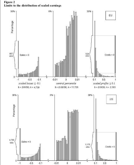
With regard to extreme observations, as explained above, we consider these to be charac-teristic of accounting data. Yet, infinancial research, it is commonplace to remove such observations as outliers even though, paradoxically, the hypothe-sised distribution is often assumed to have infinite tails.17 In contrast, a density with known support, such as that of Scaled EarningsE0, does not justify the elimination of data that lie close to the tail-end. ForE0, the true extremities lieexactlyat the limits of the function, that is, atE0=–1 where Sales=0 and at E0=1 where Costs=0. Figure 2 shows the extent of the concentration of the pooled dataset at these limits, highlighting the observations with zero Sales on the left (807 for the EU and 4,799 for the US) and
those with zero Costs on the right (524 for the EU and 1,176 for the US).18 For further analysis, we exclude these observations as they representfi rm-years with truly extreme reporting behaviour. Indeed, with regard to parametric density fitting, they represent data points that make no contribution to the surrounding local variability and therefore are an artificial source of multi-modality.
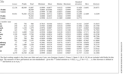
The final working sample comprises 53,087 firm-year observations for the EU and 134,234 for the US. Table 1 provides summary statistics, both for losses and for profits. In each location, the standard deviation of losses (0.2308 in the EU and 0.2772 in the US) can be seen to be far greater than that of profits (0.0521 in the EU and 0.0651 in the US). Figure 2 helps us to understand why it is that losses are more variable than profits. The bounded transformation of Net Income into Scaled Earnings reveals that losses are inclined to populate their entire permissible region, while this is not the case with respect to profits. Indeed, wefind that there is only a very small likelihood that E0 might exceed 0.5, at which point Sales would be more than three times larger than Costs. This asymmetry in the tails is reflected in the distribution of losses and profits around zero, as shown in Figure 2 by the frequencies in the central percentile. By looking more closely in the vicinity of zero in this way, it is clear that what has been characterised previously as a shortfall in small loss observations appears to be attributable to asymmetry defined by point zero, which is consistent with the fact that the tail densities are much greater for losses than for profits. This asymmetric tendency is further reflected in the medians for losses and for profits reported in Table 1 (EU median loss 0.0433, median profit 0.0223; US median loss 0.1009, median profit 0.0264).
Table 1 also gives a breakdown of the EU sample by member state, based on the location in which each of thefirms is domiciled. In most of the smaller sub-samples (Austria, Finland, Greece, Ireland, Luxembourg and Portugal), wefind that the min-imum and/or the maxmin-imum of observed Scaled Earnings is far from the respective sample limit of either 0.9999 or 0.9999 (i.e. excluding zero Sales and zero Costs). In the larger jurisdictions, however, criterionb¼ ð0:9=N1=5Þ6min s;IQR=1:349
f gwhereσis the sample standard deviation and IQR the inter-quartile range (Silverman, 1986; Salgado-Ugarte et al., 1995).
16
We also excluded a number of observations relating to German firms that habitually reported zero Net Income by adjusting their depreciation expenses and reserves accordingly. In this respect, 127firm-year observations relating to 32firms domiciled in Germany were deemed not to be usable. Degeorge et al. (1999) point out that break-evenfirms such as these will emphasise the discontinuity at zero, as scaling disperses non-zero earnings observations but not those which are exactly non-zero. 17It is shown elsewhere, in McLeay and Trigueiros (2002) and Easton and Sommers (2003), for instance, that the deflation of earnings commonly leads to a number of extreme observa-tions which, once removed, give way to other observaobserva-tions that take their place as new outliers. Indeed, Easton and Sommers (2003) examine the multivariate distribution of market capital-isation, book value and net income andfind that up to 25% of the sampling distribution would have to be removed to deal with the statistical problems arising from outliers.
18The number of
firms reporting zero Costs at least once is as follows: EU 212, US 797; more than once: EU 102, US 207. Those reporting zero Sales at least once is: EU 331, US 1,785; more than once: EU 170, US 1,019. The reporting of zero Costs appears to be unrelated to corporate domicile or industry, whereas this is not the case for zero Salesfirm-year observations (i.e. in mineral, oil and gas extraction [SIC 1000–1499]: EU 385, US 1141; in pharmaceutical preparations, medicinal and biological products [SIC 2830–2839]: EU 69, US 856).
354 ACCOUNTING AND BUSINESS RESEARCH
where markets are deeper and data are not sparse, the frequencies of Scaled Earnings tend to cover the full range. It can be seen from Table 1 that the skew estimate is consistently negative in the larger jurisdictions, at levels that reflect the estimate of 3.6691 for the EU sample as a whole. Finally, the
kurtosis of the observed frequencies is high in all sub-samples, reflecting not only the concentration around the mean but also the finiteness of tails, particularly for profits (see Balanda and MacGillivray, 1988). Allowing for the distorting effect of small sub-sample size on some estimates,
Figure 2
Limits to the distribution of scaled earnings
Note:They-axis labels indicate the number of observations at the limits of the function (i.e. EU zero Sales 807, EU zero Costs 524; US zero Sales 4,799, US zero Costs 1,176). Each histogram is plotted from nfirm-year observations, with bin width b and 30 bins. The origin for each histogram is set to the left-hand limit.
Table 1
Final sample and summary statistics
Pooled for
Observations Summary statistics for scaled earnings
1985–2004
Losses Profits Total Minimum Mean Median Maximum
Standard
deviation Skew Kurtosis
EU 12,138 40,949 53,087 –0.9999 –0.0077 0.0152 0.9999 0.1420 –3.6691 24.4571
EU Profits 40,949 0.0005 0.03404 0.0223 0.9999 0.0521
EU Losses 12,138 –0.9999 –0.1486 –0.0433 –0.0000 0.2308
US 55,931 78,303 134,234 –0.9998 –0.0712 0.0074 0.9999 0.2299 –2.1689 8.3259
US Profits 78,303 0.0000 0.0433 0.0264 0.9999 0.0651
US Losses 55,931 –0.9998 –0.2315 –0.1009 –0.0000 0.2772
EU, by member state
Austria 192 756 948 –0.7815 0.0184 0.0112 0.9015 0.1161 2.8207 33.5815
Belgium 250 914 1,164 –0.9503 0.0088 0.0124 0.9999 0.1098 –1.4882 45.3789
Denmark 249 1,230 1,479 –0.9976 0.0087 0.0154 0.9559 0.1037 –4.6065 54.6666
Finland 165 775 940 –0.9995 0.0127 0.0152 0.3309 0.0658 –5.5759 76.7922
France 1,519 6,009 7,528 –0.9920 0.0064 0.0138 0.9819 0.0966 –3.7171 46.3569
Germany 1,320 4,448 5,768 –0.9968 –0.0034 0.0076 0.9918 0.0894 –4.0841 43.4740
Greece 134 716 850 –0.9078 0.0274 0.0240 0.7055 0.0842 –0.3889 40.7506
Ireland 258 708 966 –0.9899 –0.0486 0.0189 0.7526 0.2201 –2.5592 9.7884
Italy 501 1,694 2,195 –0.9996 0.0073 0.0135 0.9999 0.0889 –4.2463 61.8068
Luxembourg 27 87 114 –0.2901 0.0236 0.0176 0.3872 0.0739 0.6656 11.8584
Netherlands 341 2,009 2,350 –0.9852 0.0119 0.0162 0.8244 0.0769 –5.9090 76.2133
Portugal 47 225 272 –0.5868 0.0174 0.0147 0.3533 0.0863 –1.6497 21.1799
Spain 184 1,177 1,361 –0.8078 0.0318 0.0210 0.9088 0.0797 0.2727 33.9162
Sweden 372 1,432 1,804 –0.9978 –0.0004 0.0172 0.9683 0.1332 –3.2069 27.2618
UK 6,579 18,769 25,348 –0.9999 –0.0221 0.0183 0.9847 0.1737 –3.2141 16.1894
Note:Thefinal working sample is free from zero Sales and zero Costs; zero Earnings (Austria 2, France 2, Spain 5, UK 8, US 26) are included with Profits for this tabulation. The measures of skew and kurtosis are non-standardised–given ther
th
central momentmr=1/nS(xi–xmean)rfori=1,2, . . . ,n, then skewness is defined as
m3m2–3/2and kurtosis as asm4m2–2.
356
ACCOUNTING
AND
BUSINESS
RESEARCH
Figure 3
Density estimation for scaled earnings, by jurisdiction
V
ol.
39,
No.
4.
2009
Figure 3
Density estimation for scaled earnings, by jurisdiction(continued)
358
ACCOUNTING
AND
BUSINESS
RESEARCH
Figure 3
Density estimation for scaled earnings, by jurisdiction(continued)
Note:The black line is the kernel density estimator ofE0defined by the Parzen (1962) kernel function with the Silverman (1986) bandwidth, the dotted curve is a normal densityN(μ,σ)fitted on the respective sampling moments (see Table 1), and the grey curve is thefitted bounded distribution. The samples are free from observations with zero Sales and zero Costs. They-axis labels indicate the maximum probability density. (0,0.25)/(0,1) and (–0.25,0)/(–1,0) indicate the percentage of non-visible profit and non-visible loss observations to the total number of profits and losses, respectively.
V
ol.
39,
No.
4.
2009
there is remarkable consistency in earnings behav-iour across the EU.
This is evident in Figure 3, which juxtaposes the three density estimators of Scaled Earnings: the nonparametric Parzen kernel estimator, the bounded distribution (solid smoothed line) and the normal (dotted smoothed line). Each of these isfitted to the EU and US samples, and separately for each of the 15 member states of the pre-enlargement EU. While estimation is applied to the entire space ofE0, i.e. [min,max] for the kernel estimator and the normal and [ξ,ξ+λ] for the bounded distribution, the graphs reproduced here focus on the interval [–0.25,0.25] in order to assist visual inspection about point zero. The consistently asymmetric shape of Scaled Earnings across the different jurisdictions is appar-ent in these plots, suggesting that Ijiri’s (1965) characterisation of the zero point in accounting earnings as the modulator of asymmetry remains valid.
This asymmetric tendency in earnings can be further understood by looking at the asymmetric tail concentration between losses and profits, as reported by Figure 3. That is, in each separate plot, the concentration of out-of-range profit obser-vations, for which E0 > 0.25 is given as a percentage of the total number of profit observa-tions, and the same approach is taken in order to calculate the concentration of out-of-range losses forE0< 0.25. It can be seen that, for both the EU and the US, the proportion of loss observations for whichE0is less than 0.25 (EU 18.9%, US 31.6%) greatly exceeds the proportion of profit observa-tions for whichE0is greater than 0.25 (EU 0.9%, US 1.5%). This pattern is repeated in all of the member states confirming that, in all jurisdictions, loss observations tend to occur throughout their entire permissible region whereas profits do not, leading us to conclude that the asymmetry around its defining point of zero is a universal property of Net Income.19
Figure 3 also shows that the unbounded normal distribution fails systematically to fit the observed frequencies, which is not surprising given the inability of the Gaussian function to take into consideration the higher order moments that are required to define the general shape of earnings. The lack of fit in the case of the US provides a good illustration of the way in which the heavier tail density for losses shifts the normal’s estimated point location downwards and away from the empirical mode. In all samples, there is considerable over-fitting in the shoulders of the distribution, which arises because the normal cannot model the high peakedness that is characteristic of earnings.20 In contrast, the bounded distribution is able to accom-modate much of the shape of Scaled Earnings, in line with the description provided by the kernel density estimator. The Lagrange Multiplier test reported in Table 2 verifies that the deviance between the fit of Equation (8) and the observed data is significantly less than in the case of the normalfit (the test is described in the Appendix).
A parametric description of the scaled earnings distribution
Table 2 gives the recovered lower boundξ, upper boundλ, scaleξ+λ, and shape parametersγ andδ, for the EU and US samples and additionally by member state of the EU. Table 2 also provides the fitted point estimates for the mean m01ðE0Þ, the median E00 and the mode E0M, as well as the standardised median value ðE00 xÞ=l¼
1þexpðg=dÞ
ð Þ 1 and the proportional distance of the median and mode from the mean
d¼ E00 m
For the bounded space of E0, the optimisation process yields exact fits to the theoretical lower bound of reporting zero Sales (E0=–1) and to the theoretical upper bound of reporting zero Costs (E0=1), both for the single European market and the US. For the smaller subsamples by member state of the EU, the parametric fits take advantage of as much of the permissible range of variation as possible, as the iterative routine simultaneously solves for all parameters. These numerical results yield bounds ofE0 that are theoretically sound, the 19
We have also applied Equation (5) to operating income and pre-tax income. The results, which are not tabulated in the paper, show that the concentration around zero and the distribution across the bounded range of variation are each sensitive to the level of income that is used. For scaled operating income, the distribution extends more smoothly to both tails and also passes through zero less abruptly. In the case of scaled pre-tax income, the inclusion of non-operating and transitory items, and prior period value adjustments, tends to increase the probability of a scaled profit and induces a more uniform allocation of scaled losses over their range. Finally, it is only with scaled net income, which takes account of all tax-related charges, plus minority interests and preferred dividend payments, that zero emerges clearly as the defining point of asymmetry inE0, with the
tax-effect mainly pulling profits away from the right-hand limit towards zero. Additional sensitivity analysis was also per-formed on the aggregation of all revenue items in addition to
sales, and the results suggest that the distributional shape of (Revenues – Expenditures) / (Revenues + Expenditures) is similar to that of the more narrowly defined (Sales–Costs) / (Sales + Costs) reported in the paper.
20
An additional test (Shapiro-Wilk-Royston), which is not tabulated in the paper, is overwhelmingly in favour of non-normality. Results by industry show that the industry factor to be much less influential than jurisdiction in shaping localised variability, with the exception of some observable differences between the cyclical and non-cyclical sectors of the economy.
360 ACCOUNTING AND BUSINESS RESEARCH
Table 2
Recovered parameters for scaled earnings
Parameters Estimates of central tendency Modelfitting
Pooled for 1985–2004
Lower bound
ξ
Scale
λ
Upper bound ξ+λ
Shape
γ δ
Mean
m01ðE0Þ
Median
E00
Mode
E0M
Standardised median ðE00 xÞ=l
Proportional distance
d%
Lagrange Multiplier
test
Optimal objective function
EU –1 2 1 –1.017 21.93 0.02317 0.02318 0.02321 0.5116 33.29 45,058.5 W-NM
US –1 2 1 –0.256 15.19 0.00843 0.00844 0.00846 0.5042 33.24 39,883.2 W-NM
EU, by member state
Austria –0.8359 1.7480 0.9121 1.382 23.37 0.01228 0.01227 0.01224 0.4852 33.29 890.83 O-NM
Belgium –0.9847 1.9847 1 –0.277 23.68 0.01344 0.01344 0.01345 0.5029 33.29 1,086.78 O-LM
Denmark –0.9979 1.9979 1 –0.765 24.69 0.01652 0.01653 0.01654 0.5077 33.30 1,427.71 O-LM
Finland –1 2 1 –0.724 22.84 0.01584 0.01585 0.01586 0.5079 33.29 849.87 O-LM
France –0.9922 1.9922 1 –0.509 23.18 0.01483 0.01484 0.01485 0.5055 33.29 7,056.75 O-LM
Germany –0.9969 1.9969 1 –0.453 32.86 0.00843 0.00843 0.00843 0.5034 33.31 5,236.61 O-LM
Greece –0.9079 1.7331 0.8251 –1.989 12.78 0.02584 0.02595 0.02615 0.5388 33.20 748.55 O-LM
Ireland –1 1.9928 0.9928 –1.248 19.85 0.02769 0.02771 0.02775 0.5157 33.28 524.92 W-NM
Italy –1 2 1 –0.564 19.41 0.01452 0.01453 0.01455 0.5073 33.28 2,002.07 O-LM
Luxembourg –0.2902 1.2902 1 6.666 5.832 0.02351 0.02173 0.01812 0.2418 33.06 87.11 D-NM
Netherlands –1 1.9791 0.9791 –1.463 25.37 0.01806 0.01807 0.01810 0.5144 33.30 2,209.19 O-LM
Portugal –1 1.9377 0.9377 –2.617 26.17 0.01724 0.01725 0.01729 0.5249 33.30 235.03 W-LM
Spain –0.8545 1.7860 0.9315 0.457 14.58 0.02454 0.02452 0.02449 0.4922 33.23 966.03 O-LM
Sweden –0.9981 1.9981 1 –0.672 20.70 0.01715 0.01716 0.01718 0.5081 33.28 1,631.73 O-LM
UK –1 1.9980 0.9980 –0.945 18.18 0.02495 0.02497 0.02501 0.5130 33.27 18,946.30 W-NM
Notes:The parameter estimates indicate whether or not the theoretical limits ofE0ξ=–1 and/orξ+λ=1 werefitted;γandδare thefitted shape parameters. The estimates of central tendency are the expected mean (first moment)m01ðE0Þ, the medianE00, the uni-modeE0M, the standardised medianðE00 xÞ=l¼ ð1þexpðg=dÞÞ 1, and the proportional distance between the point location estimatesðE00 m01ðE0ÞÞ=ðE0M m01ðE0ÞÞwhich is positive when the median falls between the mean and the mode. The Lagrange Multiplier test, which examines the null that thefit of the bounded model to the observed data is the same as thefit of the normal to the same data, asymptotically converges to thew2
2distribution with 2 degrees of freedom (allp-values are found to be less than 0.0001). Thefinal column indicates the optimal
objective function for the particular sample (ordinary, weighted or diagonally weighted least squares), and whether the Levenberg-Marquardt (LM) algorithm was successful infinding the optimal solution or gave way to the Nelder-Mead (NM) algorithm for thefinal convergence. Most samples arefitted by minimising either the O or the W objective functions, except Luxembourg which is distributed within a much narrower range of variation with significant weight in both tails and requires diagonally weighted least squares.
V
ol.
39,
No.
4.
2009
solution being independent from data points with exact contact at the limits (as noted earlier, we exclude observations withE0=–1 andE0=1).
We use the standardised median value ðE00 xÞ=l¼ð1þexpðg=dÞÞ 1 to compare the entire set of parametric fits fx;l;g;dg across samples. The standardised median represents a sigmoid (or standard logistic) function ofγandδ, with range [0,1] and a cut-off point of
1þexpðg=dÞ
ð Þ 1=0.5 when γ/δ=0. That is, for γ=0 thefitted distribution is symmetric. In the case of positive skewness, ð1þexpðg=dÞÞ 1→0 as γ/δ→∞, while for negative skewness,
1þexpðg=dÞ
ð Þ 1→1 as γ/δ→–∞. The
standard-ised median estimates are remarkably similar, with the exception of three relatively small member states which have positive γ (Austria 0.4852, Luxembourg 0.2418, and Spain 0.4922). For these jurisdictions, positiveγseems to be appropriate and simply reflects the range of their observed values which, in contrast to the other subsamples, range further over profits than losses (Austria: min=– 0.7815, max=0.9015; Luxembourg: min=–0.2901, max=0.3872; Spain: min = 0.8078, max=0.9088). The fitted mean, median and mode reported in Table 2 are more robust than their nonparametric counterparts reported in Table 1, the sample mean and the sample median. Appropriately, thesefitted estimates are always positive, consistent with the sign of expected earnings in a viable economy, and the median always falls between the mean and the mode and thus reflects the continuous unimodal density that has been proposed. In contrast, the sensitivity of the arithmetic average to extreme values in the sample can be seen to lead to negative sample means in both the EU (–0.0077) and US (–0.0712).21This is a severe shortcoming of relying on nonparametric estimates – given the consider-able number offirms and years involved, it would be implausible that the most likely expected value of earnings, in either the EU or the US, would be a loss.
The fitted estimates of central tendency also explain how the different tail weights give rise to
high density just above zero and negative skew. This is a consistent result that becomes particularly evident when we look at d, the distance of the median from the meanE00 m01ðE0Þexpressed as a percentage of the distance of the mode from the meanE0M m01ðE0Þ. This must be positive when the median of a distribution falls between the mean and the mode. Two inferences may be drawn from the analysis of the proportional distance. First,
E00 m01ðE0Þ
andE0M m01ðE0Þ
are always very small (i.e. a difference is only observed at the fourth decimal place), which reflects the high concentra-tion just above zero as well as the expectaconcentra-tion that the most likely value is indeed a small scaled profit. Second, there is a remarkable similarity in propor-tional distance across subsamples, consistently estimated close to 33%. In other words, the distance between the mode and the median is twice as large as the distance between the median and the mean in all cases, even for subsamples that are positively skewed, with expected concentration just above zero following a consistent pattern throughout.
The model fitting diagnostics reported in the final columns of Table 2 provide compelling support for the Johnson transformation. The Lagrange Multiplier test strongly favours the fit
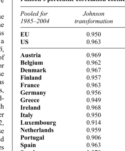
Table 3
Filliben’s percentile correlation coefficient
Pooled for
Notes:The critical values are interpolated from Vogel (1986) as follows:normal distribution: 0.978 (0.1%), 0.979 (0.5%), 0.981 (1%) 0.987 (5%);extreme value (Type I) distributions: 0.949 (0.1%), 0.952 (0.5%), 0.960(1%), 0.978 (5%).
21
Thefitted distributions comply with the Dharmadhikary and Joag-dev (1988) conditions, under which the median must fall between the mode and the mean for afinite continuous unimodal distribution (see also: Basu and DasGupta, 1997; Bickel, 2003). These conditions ensure that mean≤median≤mode under negative skewness, and that mean≥median≥mode under positive skewness (as with the three EU sub-samples of Austria, Luxembourg and Spain). This relationship does not always hold for the sample mean and median, simply because these are nonparametric results that are highly sensitive to any form of abnormality (e.g. Greece mean=0.0274
> median=0.0240 but skewness=–0.3889; Netherlands mean=0.0174>median=0.0147 but skewness=–1.6497).
362 ACCOUNTING AND BUSINESS RESEARCH
of the bounded model to the observed data over the fit of the normal to the same data (all p-values are found to be less than 0.0001). The test, which is specified in the Appendix (Equation A5), con-verged on an optimal solution using standard techniques in all cases except for the Luxembourg subsample, which is by far the smallest (N=114) and which is distributed empirically within a much narrower range of variation. Finally, indicative goodness-of-fit statistics for the Johnson trans-formation and the normal are documented in Table 3, using an extension of Filliben’s quantile-quantile correlation test. Standard goodness-of-fit measures are designed for relatively small rando-mised samples, whereas the commercial data sets that are common in accounting research provide population coverage, and therefore tend to be very large. They require a different approach, especially in order to compare across jurisdictions. Hence the use here of the Filliben correlation test. If the sample is distributed as hypothesised, we expect the relation between the ordered cumulative distribution function (CDF) to be linear with respect to the theoretical CDF, and similarly for the ith order statistics. In this case, the product moment correlation between the percentiles of the empirical cumulative frequencies and the theor-etical cumulative frequencies provides the appro-priate statistic, which has the advantage of being applicable to distributions other than the normal (Vogel, 1986; Heo et al., 2008). The results of this indicative test show high association with the best-fitting Johnson transformation (average 0.95, min-imum 0.91) and much lower association with the fitted normal (average 0.61, minimum 0.45). Indeed, in all cases except the two smallest samples, the hypothesis that the observed data fits the Johnson transformation cannot be strongly rejected, whereas for the normal distribution the hypothesis is rejected outright.
The goodness-of-fit tests indicate the appropri-ateness of the models that are fitted, and the parametric analysis set out above validates our claims for a consistently asymmetric shape of earnings that is chiefly described by negative skewness and high levels of concentration just above zero. On the whole, there is little difference in the shape of fitted densities across samples. More specifically, it is shown how asymmetry in scaled earnings is primarily defined by a longer tail for losses and a shorter tail for profits, with zero acting as Ijiri predicted, modulating the downwards pres-sure not only on profits, which is evident in the high density just above zero, but also on losses resulting in lower concentration just below zero.
Is the asymmetry about zero afirm-specific effect? Finally, we provide evidence that suggests that the asymmetry in earnings may be a feature that is predominantly introduced through firm-specific heterogeneous effects. The income of firms in a competitive environment will be attributable to the characteristics of each entity but conditional in each case on thefirm’s relationship with the rest of the market. If markets are complete, with perfect information and homogeneity in the allocation of resources, the reportedfirm profit in this frictionless universe will be absent of incentives and other stimuli that create asymmetry. We anticipate there-fore, that once we remove the fixed effect that definesfirm-specificity, we will induce approximate symmetry about zero. The standard approach in panel methods is employed here, whereby the arithmetic averages for each panel (in this case a firm) are thefixed effects. Such effects are described in modern microeconometric analysis as either unobserved or unobservable, and they characterise the between-panel heterogeneity in the pooled sample (e.g. Cameron and Trivedi, 2005).
To examine this proposition, consider a more comprehensive description of Scaled Earnings E0
withfixed attributes for eachfirmi, for each of the sectors s in which the sampled firms operate, for each of the jurisdictions j in which they are domiciled, and for each yeart. Thefixed attributes are thus thefirm meanĒ0
ifori=1,2, . . . ,n, the sector meanĒ0
s wheresdenotes a two-digit SIC class, the jurisdiction meanĒ0
jwherejdenotes an EU member state, and the year-by-year mean Ē0
t for each t=1985,1986, . . . ,2004. By subtracting the arith-metic average of the earnings stream with respect to any one of these attributes, we effectively eliminate the expected heterogeneous effect that is associated with that particular trait. We then repeat the Parzen-kernel estimation procedure with the mean-adjusted data, in order to assess which, if any, of these characteristics may cause the distribution to deviate from symmetry.
Panel A of Figure 4 contrasts the kernel density estimators of the pooledfirm-year sample of Scaled EarningsE0 with the densities of observations that are mean-adjusted by firm E0 Ē0i mainly interested in observing the distribution of earnings around zero, the graph focuses on the centralfive percentiles, i.e. over the range [–0.025, 0.025]. The effect is very noticeable in both the EU and the US, suggesting that heterogeneity across firms is the main cause of asymmetry in the pooled samples. By comparison with the pooled data,
Figure 4
Panel A: Asymmetry in earnings is afirm-mean effect
Note:The kernel density plots above focus on the central 5% [–0.025,0.025]. The estimates for the pooled unadjusted Scaled EarningsE0are plotted together with those for the mean-adjusted values byfirmE0 Ē0i
, by sectorE0 Ē0s
, by yearE0 Ē0t
and, for the EU only, by jurisdictionE0 Ē0j
. The data set comprises of 53,087firm-years in the EU and 134,234 in the US. The table above gives the standard deviations for each of the unadjusted and mean-adjusted samples, together with the Levene Test for Homogeneity of Variance, which is a robust test for examining the null of equality in variances between non-normal frequencies, and follows anF
distribution with (1,N–2) degrees of freedom.
364
ACCOUNTING
AND
BUSINESS
RESEARCH
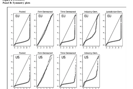
Figure 4(continued)
Panel B: Symmetry plots
Note:The symmetry plots above show the distance from the median of the observed distribution, i.e. they-axis measures the distance above the median and thex-axis measures the distance below the median. The plot region has been restricted to the interval [–1,1] for both axes.
V
ol.
39,
No.
4.
2009