Gadjah Mada International Journal of Business January-April 2010, Vol. 12, No. 1, pp. 117–133
Insukindro
Professor of Economics, Faculty of Economics and Business, Universitas Gadjah Mada, Yogyakarta, Indonesia
Gumilang Aryo Sahadewo
Graduate student, Department of Economics, Boston University, U.S.
A series of relatively high inflation characterize Indonesian economy, especially during the economic crisis. Economists generally agree that high inflation is one of the major economic problems, and that economic authorities need to cope with such a problem. Therefore, it is essential to understand the behavior of inflation in Indonesia. The aim of this paper is to estimate the inflation dynamics in Indonesia using equilibrium correction and forward-looking Phillips Curve approaches. Previous em-pirical studies show that the equilibrium correction or back-ward-looking approach may explain the inflation dynamics in Indonesia. The backward-looking specification does not have to be the proper model even if the fact shows that the specifica-tion holds. The major innovaspecifica-tion of this paper is the applicaspecifica-tion of a forward-looking Phillips curve model. The empirical re-sults—estimated using the Generalized Method of Moments
INFLATION DYNAMICS IN INDONESIA:
EQUILIBRIUM CORRECTION AND
FORWARD-LOOKING
PHILLIPS CURVE APPROACHES*
* Earlier draft of this paper was presented in a seminar organized by the Master of Science and Doctorate Programs, FEB UGM, Yogyakarta on March 2, 2010, in the GSICS Development Seminar at Kobe University, Japan on March 12, 2010; and in the 191st IDEC Asia Seminar at Hiroshima
Keywords: equilibrium correction; forward-looking; GMM; inflation; Phillips curve JEL Classification: C22, C51, E31
(GMM)—show that the forward-looking Phillips Curve ap-proach dominates the backward-looking behavior. It indicates that after a credible monetary policy announcement, for in-stance, the former model predicts that economic agents will change their behavior quickly. Therefore, the policy will affect the economy more rapidly.
Introduction
Inflation phenomenon in Indone-sia is unique compared to that in other Asian countries due to the involvement of numerous contributing factors. In addition, the movement of inflation dur-ing economic crisis is typical. The col-lapse of banking sector led to financial breakdown, political turmoil, lengthy spell of drought, tight monetary policy, oil prices hike, and international eco-nomic crisis; all contributed to the high inflation in Indonesia. The aforemen-tioned phenomena basically stem from a starting point, which is the behavior of agents in the economy. Study on agent behavior in relation to inflation is essen-tial since agent behavior is directly influenced by the agent’s expectations. It is also motivating to observe inflation dynamics in Indonesia given its nature as a developing country. The emblem-atical imperfection of information and problematic institutions in Indonesia fundamentally influence agent behav-ior and eventually agents’ expecta-tions.
For more than half a century, Phillips Curve has stimulated numerous aca-demic debates and inquiries among economists. The debates have sparked discussion on key macroeconomic vari-ables influencing inflation dynamics or on agent behavior toward inflation, i.e., agents’ expectations. Neoclassical economists argue that expectations are backward-looking whereas New Clas-sical economists suggest that expecta-tions are rational, thereby forward-looking (Whelan 2005). Later on, the new breed of macroeconomic theory, New Neoclassical Synthesis (hence-forth NNS), integrates rational expec-tations as one of its basic elements (see for examples Goodfriend and King 1997; Goodfriend 2004, 2008; Zouache 2004; and Giese and Wagner 2007 for further discussion on NNS).
Vamvakidis (2002) show that base money and productivity as well as ex-change rate and foreign inflation are the key indicators of inflation in Indo-nesia. Adrison (2002) studies the ef-fects of government expenditures and money supply shocks on Indonesian economy. He notes that money supply shock does not significantly influence output and inflation. Hossain (2005) finds that there exists a long-run causal relationship between money supply growth and inflation.
Anglingkusumo (2005) employs several P-star models, including a simple Markov-Switching P-star model, to verify that inflation is always a mon-etary phenomenon in the long run. He
finds that excess money supply (M1)
traces the long-run dynamics of CPI inflation very well. He also notes that changes in inflation are determined by the excess of money shocks and peri-odic price adjustments to eliminate such shocks in the period of crisis. He con-cludes that money still acts as the prime mover of inflation even when expecta-tions are stable. Puzon (2009) studies the inflation dynamics in ASEAN-4 countries (i.e., Philippines, Thailand, Malaysia, and Indonesia), and also finds that the control variables of inflation in the countries in question are different. Previous empirical studies dis-cussed above have successfully ex-plained the behavior of inflation dy-namics in Indonesia. We should note that those studies generally applied the equilibrium correction or the error cor-rection or the backward-looking ap-proaches to their econometric
analy-ses. Price and Insukindro (1994) argue that even if such specification holds, it does not necessarily imply that the proper model is backward-looking.
The main purpose of our study is to analyze the nature of expectations in inflation dynamics in Indonesia. We aim to explain the formation of agents’ expectations that determine the infla-tion dynamics and to construct back-ward- and forback-ward-looking models. We will also employ the equilibrium correc-tion model with shock variable since some previous studies observe the im-portance of money supply shock to inflation (see Anglingkusumo 2005; Khan and Moessner 2004).
This study yearns to present the insights into inflation dynamics that are consistent with recent development of forward-looking Phillips Curve. There will be different policy implications since backward- and forward-looking hold opposing behaviors. A credible policy will be exercised immediately into agents’ decision-making if the for-ward-looking framework holds. Agents, on the other hand, will wait for data realization before making any de-cision if backward-looking framework prevails (see also Price and Insukindro 1994). Policy will take more time to have effects if the backward-looking framework holds rather than the for-ward-looking framework.
research. The final Section presents our conclusion.
Review of Related Literature
Philips Curve (1958) originally estimates a negative relationship be-tween nominal wage inflation and un-employment in the U.K. Since then, it has played an essential role in explain-ing the inflation dynamics in economy. The ongoing debate on inflation dy-namics, mainly in the New-Keynesian Phillips Curve (NKPC) framework, is whether forward-looking behavior has the ability to explain inflation. The model of NKPC shows that inflation is deter-mined by the expectations of future inflation and a driving variable such as real marginal cost, output gap, or un-employment.
Results of various studies offer mixed verification. Galí and Gertler (1999) establish the so-called “hybrid model” in which backward- and for-ward-looking behaviors are integrated to estimate the NKPC. Real marginal cost is used instead of output gap as the forcing variable of inflation, and infla-tion is assumed to be the present-value of expected future real marginal cost. They confirm that forward-looking behavior is an important measure of inflation in the U.S. via the hybrid model. The study also shows that the backward-looking behavior is not quan-titatively important despite its signifi-cance. Galí et al. (2001) observe infla-tion in Euro countries and prove, albeit not as the main objective of the study, that inflation is influenced by
forward-looking behavior. Later on, Tillmann (2005) uses a distinct model to reveal that inflation in U.K. is the realization of expected future real marginal cost; accordingly, inflation is forward-look-ing.
Several studies disagree that for-ward-looking specification has the abil-ity to explain inflation. Rudd and Whelan (2001) find that the present value of expected future driving variables, out-put gap and real marginal cost, could only explain a small portion of actual inflation. A number of studies consider that the test of hybrid model is rather weak compared to the non-nested back-ward-looking specification (see also Rudd and Whelan 2003; Bardsen et al. 2005; and Dorich 2009 for more dis-cussion on this issue).
Our study enters the debate by estimating the inflation dynamics with a forward-looking specification, and tests such specification with a back-ward-looking one to observe which model specification is superior to ex-plain the inflation dynamics in Indone-sia. We turn to model specification and testing in the next section.
Model Specification
(see Williamson 2008: Ch. 17). We shall note that the expected sign of the parameter when using output will be different from that of unemployment. Assuming log linearity, we can write the price equation in period t as follows.
where x are the driving variables (a vector of variables influencing price). Equation (1) explains the long-run or equilibrium relationship between price level and its driving variables. How-ever, economic systems are often drifted away from the equilibrium (Tho-mas 1997: 383). It is generally argued that economic agents will find that the
actual pt will diverge from the planned
or desired pt*. The divergence may be
caused by shock variable and subse-quent slow adjustment. Therefore, in this case, we also assume that agents attempt to minimize the following qua-dratic loss function (Domowitz and Elbadawi 1987; and Insukindro 1992).
where
Hence, substitute equation (3) into (2), and we can write (2) as
where is short-run planned pt and
is desired or long-run ptand ztis a vector of variables influencing pt* and
j is a row vector that weights each
element of zt. Variables st and L are shock variable and lag operator, re-spectively. The first component of loss function (4) represents the disequilib-rium cost, which is the cost of being away from static equilibrium, whereas the second one is the adjustment cost.
The parameters and are the
weights on which the agents place the disequilibrium cost and the adjustment cost, respectively.
We can solve and reparameterize equation (4) to yield the following Equi-librium Correction Model or Error Cor-rection Model (ECM) with shock vari-able [to derive equation (5), see Insukindro (1992, 1998)].
We shall make assumptions be-fore we establish the forward-looking specification. Domowitz and Elbadawi (1987: 262) state that in a fully rational world, the behavior of an individual agent is generally assumed to be estab-lished in reference to an infinite dis-counted sum of his or her expected value of the loss function. We assume that forward-looking agents are ex-pected to minimize the following loss function (see Cuthbertson 1988; Price and Insukindro 1994; and Koutsomanoli-Filippaki et al. 2008).
We use Sargent’s method of for-ward operators as shown in Sargent (1979, Chapter IX) to construct the forward-looking specification below.
Equation (7) has only two param-eters, which are the coefficient on the
lagged dependent variable, , and the
discount factor, D. E denotes the
con-ditional expectation based on all
infor-mation available at time t. The
coeffi-cient of is associated with the speed
of adjustment. We must note that the
values of the optimal price level or p*
are unobservable, thus we will solve this situation in the estimation. We utilize the forecast of preferred
meth-ods for the values of p* before we
incorporate them into our model. We may write (7) as
Time series data are stochastic in general, hence time series analysis oblige researchers to observe the na-ture of the data before moving on to estimate the specification. The fore-most step in acquiring necessary infor-mation containing the nature of the data is the inference on the data order of integration. We should examine whether the data are integrated of
order zero, I(0), or integrated of order
one, I(1). We employ the standard
Augmented Dickey-Fuller (ADF) and Phillips-Perron (PP) to test the data order of integration.
We may employ several estima-tion methods, such as autoregressive distributed-lag (ARDL) model, Partial Adjustment Model (PAM), and Shock Absorber Model (SAM). We should note that data are usually stochastic or
I(1), hence estimations with the
mum likelihood test of cointegration as revealed by Johansen (1988) if we are uncertain about the underlying theory of variables’ relationships.
We may also find another phe-nomenon that has a different order of integration of the estimated variables. We may not use the methods above since the condition is that the variables are integrated in the same order whether it is I(0) or I(1). We may argue that the estimation of I(0) and I(1) variables altogether will generate a phony relationship. Pesaran and Shin (1995) find an answer to such a quan-dary by proposing the ARDL approach to cointegration. The proposed ap-proach is capable of testing the cointegrating relationship between I(0) and I(1) or even mutually integrated variables.
We shall decide on the class of estimator to be used in the estimation of the specifications. The extensively used OLS method has some disadvantages as it is inept in the estimation of non-linear parameters as well as non-non-linear rational expectations model. Hansen and West (2002) reveal that the esti-mator of Generalized Method of Mo-ments or GMM can solve a model with linear variables but subject to non-linear restrictions on the parameters. Wooldridge (2001) argues that GMM is proficient in estimating a sophisti-cated non-linear rational expectation model, and reveals that such estimator takes into account of serial correlation of unknown forms as well as heteroscedasticity. Hansen and West (2002) and Verbeek (2008:161) affirm
the argument by noting that GMM does not require a parametric model for conditional heteroscedasticity or any distributional assumption. Our study chooses the best approaches based on the nature of our data as well as our model. We aim to establish a robust model to explain the inflation phenom-enon in Indonesia.
Monetary Variable Shock
Khan and Moessner (2004), and Adrison (2002) and Anglingkusumo (2005) observe that monetary shock is essential in price determination in the U.K. and Indonesia, respectively. Our constructions of equilibrium correction specifications include such shock vari-able. We integrate short- and long-run shocks in the backward-looking speci-fication since it is assumed that the movement of money supply is persis-tent in influencing price.
We employ the Box-Jenkins meth-odology framework to estimate the best ARIMA model of money supply
(M2) in Indonesia. We use the
residu-als of the ARIMA model as the proxy for the shock variable. We apply this method in the light of Insukindro (1998)
who applied the residuals of AR(2) and
the deviations of reserve money from its linier trend as the proxies for shock variable in question.
Forward-Looking Specification
ob-servable. We may employ, for ex-ample, Kalman Filter, Hodrick-Prescott Filter, and the fitted values of the cointegrating or equilibrium equation in the ECM estimation to estimate the optimal price level. We choose the fitted values of long-run equation in ECM since it may generate a long-run path. The method undertaken above has been applied by Price and Insukindro (1994), but not in the context of infla-tion dynamics in Indonesia and the employment of GMM.
The expected future price level
E(pt+s) will vary from pt+s by a white-noise random error in the forward-looking specification. We can state that the variable is correlated to the error term. The orthodox solution of such occurrence is to estimate the model using instrumental variables. The variable is initially regressed on the instrumental variables to get rid of the correlation with the error term. The system will then use the fitted values of the regression to estimate the intended specification.
We may employ several classes of estimators such as two-stage least squares (2SLS), non-linear least squares (NLLS), and GMM to esti-mate our specifications using instru-mental variables. We opt to employ the GMM since our specifications assume non-linear parameters as well as ratio-nal expectations in the optimization of the model.
Non-Nested Test
We test our forward-looking speci-fication against the alternate hypoth-esis of backward-looking specifica-tion. Equations (5) and (7) may not be regarded as a nested version of one another, hence they are considered non-nested models. The general test used extensively in testing an alternate hypothesis in non-nested models is Davidson-McKinnon’s J-test (Mc Kinnon et al. 1983).
We summarize our econometric methodology to estimate the specifica-tions in the previous section. Initially, we estimate the long-run or coin-tegrating parameter. Next, we esti-mate the dynamics using the appropri-ate method for our backward-looking specification. We then estimate the forward-looking specification and com-pare it with the backward-looking by employing the Davidson-McKinnon’s J-Test.
Empirical Results
Data
(2010). We use money supply (M2) to generate the proxy for monetary shock, which will later be incorporated into our backward-looking model.
Figure 1 shows that for the last decade, the inflation rate in Indonesia has been relatively volatile, except in its economic crisis of 1998. Inflation rate accounted an average of 1.705 percent per quarter or roughly 6.82 percent per annum during the period of 1993(I)-1997(III). The inflation rate after the crisis, between 1998 and 2007, was steady at an average of 1.77 percent per quarter.
Indonesia suffered from a high inflation rate, reaching 16 percent in the fourth quarter of 1997 and stretched to a peak of 50.88 percent in the first quarter of 1998. The inflation rate rose to an average of 11.97 percent per
quarter during the period of 1998 crisis, between 1997(IV) and 1999(III). The inflation rate reached an average of 2.27 percent between 1999(IV) and 2005(III), which was higher than the average inflation rate before the 1998 economic crisis.
Inflation rate in 2005(IV) reached 10.84 percent since Indonesia was faced with increases in gasoline prices that affected production costs. Oil cri-sis in the beginning of 2008 also drove the inflation to a rather high average of 5.45 percent per quarter. The high inflation rate has since decreased sub-sequent to the global slowdown set off by financial crisis. Inflation rate even-tually increased in the second and third quarters of 2009 as the economy re-covered.
Figure 1. Inflation in Indonesia (in percentage): 1993(I)-2009(III)
Order of Integration
The first and foremost step in our estimation is the test of variables’ order of integration. Our estimation of Indo-nesian inflation dynamics incorporates
wholesale price index (Pt) and GDP
(Yt). We employ ADF and PP for the
test, and the results are given in Table 1.
The results of ADF and PP tests show that all variables are integrated of order one; in other words, the variables are not stationary in level. A possible approach to estimating our backward-looking specification given the nature of the data above is the Engle-Granger ECM.
Backward-Looking
Specification
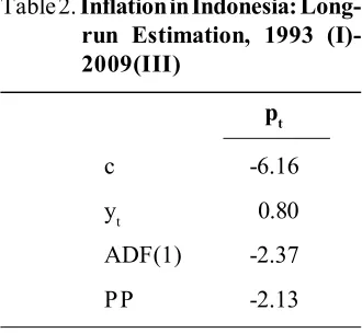
We employ the Engle-Granger ECM to estimate the inflation dynam-ics in backward-looking framework. The first step of the Engle-Granger ECM is to verify the cointegrating relationship between variables. Table 2 shows the cointegrating relationship between p and y.
Readers and analysts might be tempted to interpret the statistics of the
long-run regression above, such as t-,
F-, and 2 statistics. The regression
above is in fact spurious since all
vari-ables are I(1). All interpretations with
Table 1. Order of Integration
Indonesia Indonesia
Variables I(0) I(1)
ADF PP ADF PP
pt 2.62 2.99 -4.94 -5.34
yt 4.60 9.37 -5.39 -9.35
Notes:Ln (P) = p and ln (Y) = y. Sample, 1993:01 – 2009:03; MacKinnon’s critical value for I(0) test, 95% = -1.94 for p and y; MacKinnon’s critical value for I(1) test, 95% = -3.48 for p and y.
Table 2.Inflation in Indonesia:
Long-run Estimation, 1993 (I)-2009(III)
pt
c -6.16
yt 0.80
ADF(1) -2.37
PP -2.13
respect to t-, F-, and 2 statistics are
consequently subject to biases. There-fore, we are not obliged to report such statistics since it may be misleading.
The possible interpretation of the regression above is the sign and the magnitude of parameter coefficient. The sign of the coefficient is positive as suggested by the theory, and the mag-nitude of the coefficient that explains the short-run effect of PDB growth on inflation is below unitary (1) as ex-pected.
Unit root tests on the residuals of the long-run regression above show that we have relatively weak evidence of cointegrating relationship between the variables. However, we may con-tinue to the second step of ECM-EG, which is the equilibrium correction es-timation.
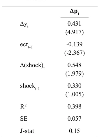
The ECM functions as our back-ward-looking specification which will later be compared with the forward-looking model. Short- and long-term money supply shocks are also included in our backward-looking specification (5). We exercise GMM to estimate the equilibrium correction specification as discussed before.
Wooldridge (2001), as previously mentioned, suggests that GMM esti-mation has already taken account of an unknown form of serial correlation as well as heteroscedasticity. Therefore, it is unnecessary to disclose the diag-nostic reports of GMM estimation above. There is a note that GMM estimation requires overidentification condition to be fulfilled, and our model
has done so. In addition, the R2 of the
estimation is respectable for the esti-mation of differences.
Table 3. Inflation Dynamics in
Indo-nesia: ECM with Shock
The ECM specification is well defined as shown in Table 3. The parameter of GDP growth has a sen-sible magnitude and is correctly signed. The error correction term coefficient
and t-statistic provide evidence of the
existence of cointegration, but the mag-nitude of the coefficient suggests a slow adjustment. There is weak evi-dence that money supply shock may have an effect on price determination in the short run but not in the long run. It may indicate that the shock is only temporary in influencing inflation in Indonesia.
Our findings in terms of short-run money supply shock basically substan-tiate previous studies. Anglingkusumo (2005) argues that the influence of excess money on inflation is not imme-diate and will be characterized by long delays. Adrison (2002) reveals that a change in money supply shock does not influence inflation rate significantly.
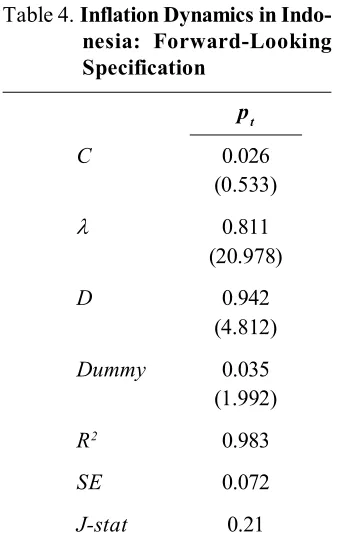
Forward-Looking Specification
The optimal value of price or pt*
makes use of the long-run parameter from the cointegrating estimation in Table 2. The lead of the optimal value is employed in the forward-looking specification.
Table 4 shows that the forward-looking specification in Indonesia is well defined in a simple dynamic equa-tion. The magnitudes of the coeffi-cients are sensible and properly signed. The computed discount factor is also reasonable as predicted in previous
studies. The values of in the
specifi-cation shows that, as expected, the speed of adjustment is faster than the result obtained in the previous back-ward-looking estimation.
Table 4. Inflation Dynamics in
Indo-nesia: Forward-Looking
Forward Versus Error
Correction Specification
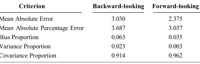
We focus on the models’ predic-tive performance by observing the bias, variance, and covariance proportion as Pindyck and Rubinfeld (1998: 387-388) suggest. We expect the values of bias and variance proportion to be near to zero, and the value of covariance pro-portion to be near to unity. A high value of bias proportion (exceeding 0.20) verifies a predictive failure of the model since it illustrates a systematic error of the model. It is also suggested that we opt for a model with the lowest mean absolute error as well as mean absolute percentage error.
The predictive performance of the forward-looking specification is better than that of the backward-looking
speci-fication as shown in Table 5. The informal analysis suggests that the for-ward-looking specification in Indone-sia outruns the backward-looking one. We must run the formal test after-wards—using the non-nested test—to decide on which model is the best.
The methodology of non-nested test is as follows. Fitted values of each specification are incorporated into the alternative specification. If the param-eter of the fitted values is significant, the null hypothesis is rejected against the alternative, and vice versa. We should take notice of the condition that the parameter coefficient should be positive in the interval [0,1], hence a one-sided test is the most suitable (Price and Insukindro 1994). The results are assembled in Table 6.
Table 5. Predictive Performance
Criterion Backward-looking Forward-looking
Mean Absolute Error 3.030 2.375
Mean Absolute Percentage Error 3.687 3.037
Bias Proportion 0.063 0.035
Variance Proportion 0.023 0.003
Covariance Proportion 0.914 0.962
Table 6. Non-nested Test
H0 H1 Coefficient t-statistics
Indonesia
Forward Backward -0.050 -0.217
The non-nested test reveals that the forward-looking specification is not rejected in favor of the backward-looking specification. Rather, the back-ward-looking specification is rejected in favor of the forward-looking specifi-cation. The results of the test conclude that the forward-looking specification is superior to the backward-looking one.
Conclusion
Indonesia possesses distinctive in-flation behavior given its nature or characteristics as a developing coun-try, such as information imperfection and problematic institutions. Indonesia is also an open economy such that internal as well external shocks may contribute to inflation determination. Thorough knowledge of the factors that influence the inflation behavior in Indonesia is then essential.
Our major contribution in the dis-cussion of inflation dynamics in Indo-nesia is the construction of equilibrium error with shock variable and the for-ward-looking specification based on the Phillips Curve and the nature of agent behavior. Our backward- and forward-looking specifications are well defined according to our expectation
as well as general theory. One of our findings, albeit not a pivotal one, is an indication that monetary shock may have a temporary effect on inflation.
Estimation results of the inflation dynamics reveal that agents seem to be forward-looking or rational. Informal comparisons as well as the formal Davidson-McKinnon J-test are per-formed between backward- and for-ward-looking specifications. Both com-parisons affirm that the forward-look-ing specification is superior to the back-ward one. The results of our estimation through non-linear models verify that the Phillips Curve is non-linear.
References
Adrison, V. 2002. The effect of money supply and government expenditure shock in Indonesia: Symmetric or asymmetric? Working Paper 02/18. Georgia State University Andrew Young School of Policy Studies
Anglingkusumo, R. 2005. Money-inflation nexus in Indonesia.Discussion Paper 054/4. Tinbergen Institute.
Bardsen, G., O. Eitrheim, E. S. Jansen, and R. Nymoen. 2005. The Econometrics of Macroeconomic Modeling. New York: Oxford University Press, Inc.
Cuthbertson, K. 1988. The demand for M1: A forward looking buffer stock model. Oxford Economic Papers 40: 110-131.
Domowitz, I., and L. Elbadawi. 1987. An error correction approach to money demand: The case of Sudan. Journal of Development Economics 26: 257-75.
Dorich, J. 2009. Forward looking versus backward looking behavior in inflation dynamics: A new test. 43rd Conference of Canadian Economics Association, downloaded from
http://economics.ca/2009/papers/0241.pdf.
Engle, R. F., and C. W. Granger. 1987. Cointegration and error correction: representation, estimation, and testing. Econometrica 55: 251-76.
Gali, J., and M. Gertler. 1999. Inflation dynamics: A structural econometric analysis. Journal Monetary Economics 44: 195-222.
Gali, J., M. Gertler, and D. V. Salido. 2001. European inflation dynamics. European Economic Review 45: 1237-1270.
Goodfriend, M. 2004. Monetary policy in the New Neoclassical Synthesis: A primer. Economic Quarterly, Federal Reserve Bank of Richmond (90/3): 21-45.
Goodfriend, M. 2008. The case for price stability with a flexible exchange rate in the New Neoclassical Synthesis. Cato Journal 28: 247-254.
Goodfriend, M., and R. G. King. 1997. The New Neoclassical Synthesis and the role of monetary policy. NBER Macroeconomics Annual: 971-987.
Giese, G., and H. Wagner. 2007. Graphical analysis of the new neoclassical synthesis. Diskussionsbeitrag: 411.
Hansen, B. E., and K. D. West. 2002. Generalized method of moments and macroeconomics. Journal of Business and Economic Statistics 20: 460-469.
Hossain, A. 2005. The sources and dynamics of inflation in Indonesia: An ECM model estimation for 1952-2002. Applied Econometrics and International Development 5 (4): 93-116.
Insukindro. 1992. Dynamic specification of demand for money: A survey of recent developments. Indonesian Economic Journal 1: 8-23.
money: A theoretical review and an empirical study in Indonesia]. Ekonomi dan Keuangan Indonesia 46: 451-471.
International Monetary Fund (IMF). 2010. International Financial Statistics. International Monetary Fund Website, downloaded January 2010 from www.imfstatistics.org/imf/ logon.aspx.
Johansen S. 1988. Statistical analysis of cointegrating vectors. Journal of Economic Dynamic and Control 12: 231-54.
Khan, H., and R. Moessner. 2004. Competitiveness, inflation, and monetary policy. Bank of England Working Paper 246.
Koutsomanoli-Filippaki, A., E. Mamatzakis, and S. Christos. 2008. European Banking Integration Under a Quadratic Loss Function. http://efmaefm.org/OEFMAMEETINGS/ EFMA%20ANNUAL%20MEETINGS/2008-athens/647.pdf.
McKinnon, J. G., R. Davidson, and H. White. 1983. Tests for model specification in the presence of alternative hypotheses. Journal of Econometrics 21: 53-70.
Pesaran, H. M., and Y. Shin. 1995. Autoregressive distributed lag modeling approach to cointegration analysis. DAE Working Paper Series (9514). Department of Applied Economics University of Cambridge.
Phillips, A. W. 1958. The relation between unemployment and the rate of change of money wage rates in the United Kingdom 1861-1957. Economica 25: 283-299.
Pindyck, R., and D. Rubinfeld. 1998. Econometrics Model and Economic Forecasts (4th ed.).
Singapore: McGraw-Hill, Inc.
Price, S., and Insukindro. 1994. The demand for Indonesian narrow money: Long run equilibrium, error correction, and forward looking behavior. The Journal of Interna-tional Trade and Economic Development 3 (2): 147-63.
Puzon, K. A. 2009. The inflation dynamics of ASEAN-4: A case study of the Phillips curve relationship. Journal of American Science 5 (1): 55-57.
Ramakrishnan, U., and A. Vamvakidis. 2002. Forecasting inflation in Indonesia. IMF Working Paper (WP/02/111).
Rudd, J., and K. Whelan. 2001. New test of the New-Keynesian Philips curve. Finance and Economics Discussion Series (52). Board of Governors of the Federal Reserve System. Rudd, J., and K. Whelan. 2003. Can new rational expectations sticky-price models explain inflation dynamics. Finance and Economics Discussion Series. Board of Governors of the Federal Reserve System.
Sargent, T. J. 1979. Macroeconomic Theory. Academic Press.
Thomas, R. L. 1997. Modern Econometrics: An Introduction. Addison Wesley. Tillmann, P. 2005. Does the forward looking Philips curve explain the UK Inflation?
Manuscript. Institute of International Economics, University of Bonn.
Verbeek, M. 2008. A Guide to Modern Econometrics (3rd ed.). John Wiley & Sons, Ltd.
Downloaded January 2009 from http://tcd.ie/Economics/staff/whelanka/topic7.pdf. Williamson, S. D. 2008. Macroeconomics. Pearson Education, Inc.
Wooldridge, J. M. 2001. Applications of generalized method of moments estimation. Journal of Economic Perspectives 15: 87-100.