as a Distributed Fixed Effect
Christopher Dougherty
a b s t r a c t
Wage equations using cross-sectional data typically find an earnings pre-mium in excess of 10 percent for married men. One leading hypothesis for the premium is that marriage facilitates specialization that enables married men to become more productive than single men. Another is that the pre-mium is attributable to an unobserved fixed effect, married men possessing qualities that are valued in the labor market as well as the marriage market. This paper suggests that the premium is attributable to an unobserved time-distributed fixed effect that emerges and grows with the approach of mar-riage and continues to grow for some years after marmar-riage. A similar distributed fixed effect is found in the case of women, but it is smaller and declines after a few years of marriage. The results appear to cast doubt on the specialization hypothesis.
I. Introduction
Virtually all studies find that married men tend to earn significantly more than single men, with estimates of the marriage premium usually exceeding 10 percent. The large magnitude of the marriage premium has important implications not just for understanding male/female wage differentials and wage discrimination, but also for understanding the determinants of individual wages, income inequality, mar-riage formation, and specialization within marmar-riage. Of the two main hypotheses put forward to account for it, one is that the effect is real, married men finding it easier to accumulate human capital, as predicted by Becker’s theory of role specialization in marriage (Becker 1973, 1974, 1981), and consequently being more productive than single men. The other is that the premium is a statistical illusion caused either by the
Christopher Dougherty is a senior lecturer in economics at the London School of Economics. He wishes to thank participants in seminars at the LSE Centre for Economic Performance and the International College of Economics and Finance, Moscow, and an anonymous referee for helpful comments. The data used in this article can be obtained beginning October 2006 through September 2009 from the author, email c.dougherty@lse.ac.uk.
[Submitted September 2005; accepted October 2005]
endogeneity of marriage to wages or by unobservable heterogeneity, more productive men possessing characteristics that make them more likely to be married. As yet there is no consensus in sight.1The present paper finds a time dimension to the emergence of the premium that appears to be more compatible with the second hypothesis than the first.
II. Methodology
For studies using panel data, such as the present one, the wage equa-tion is typically of the form
(1) lnYit
冱
X Mj j jit it i it = b +m +a+f
where Yitis a measure of earnings, the Xjitare the intercept and observed correlates other than marital status, Mitis an indicator of marital status, αiis an unobserved individual-specific term picking up the effect of unobserved correlates, and εitis an idiosyncratic error term. i, j, and tindex over individuals, the observed correlates, and time periods, respectively. Averaging the data for each individual over time periods,
(2) lnYi
冱
X Mj j ji i i i
= b +m +a+f
-Subtracting this from Equation 1, one obtains
(3) ln(Yit Yi)
冱
(X X) (M M) ( )j j jit ji it i it i
- = b - +m - + f -f
-and the unobserved fixed effects are washed out, along with the intercept -and any time-invariant observed correlate.
A potential problem with this approach, not previously discussed in the literature on the marriage premium, is the restrictive assumption that the fixed effects are truly fixed. Casual observation suggests that, while some character traits are determined early on in life, others are susceptible to modification. In particular, the priorities and behavior of young people are often very different from those of the more mature adults into whom they are eventually transformed. Indeed the very notion of matura-tion implies a process of change in which attitudes and values adjust in the direcmatura-tion of socially approved norms. Marriage may be one of the outcomes of this process, not only because potential spouses find characteristics associated with maturity attractive, as has often been suggested in the literature, but also because the maturing individual may become readier to commit to the institution. An increasing seriousness of purpose concerning work may be another outcome. If this is the case, an index of maturity should be positively associated with earnings and its effect should be expected to grow during the transition from immaturity to maturity. Given an association between matu-ration and marriage, one would expect the impact of the index of maturity on earnings to be discernible some time before marriage, for it to increase as the time of marriage approaches, and possibly for it to continue to increase for some time afterwards.
To fit such a model without prespecifying the form of a maturation function one may replace the marriage dummy variable Mit in Equation 3 by a set of dummy
variables Mit pwhere
pis the number of years since marriage, if positive, and the number to marriage, if negative. If the maximum horizon forwards or backwards from the time of marriage is syears, the distributed marital effects model may be written
(4) m M +a +f
There is, however, an unavoidable technical problem when fitting this model using fixed effects. Consider the simplified model
(5) lnYit
冱
X MARRIESj j jit it i it
= b +m +a +f
where MARRIESitis equal to one if the individual ever marries and zero otherwise. Because MARRIESitfor individual iis constant over all time periods, being equal to zero in the case of those who never marry, and one for those who at some time do, it drops out when the model is fitted using fixed effects. The same is true for Equation 4, since the Mit
pare a disaggregation of
MARRIESit, with
Hence the contrast with being single is lost. However if it is argued that, for large enough s, λ–sis close to 0, implying that an individual with syears to marriage is no different in maturity from an individual who never marries, then the fixed effects model may be fitted dropping Mit
s
- .
III. Data
The data are taken from the National Longitudinal Survey of Youth 1979–, a survey that has been fielded annually from 1979 to 1994 and at biennial intervals since 1994. The sample is restricted to respondents in the core NLSY sam-ple. Marital status data are taken from all the waves from 1980 to 2002. Earnings data are taken from all the waves from 1980 to 19982and are adjusted to 1996 prices using the CPI—Urban price index. Observations are restricted to respondents not enrolled in school, not employed in an odd job, working at least 30 hours per week, earning at least $2.50 per hour and not more than $250 per hour at 1996 prices, and either sin-gle or married. The sample consists of 20,187 observations on 2,466 males and 14,781 observations on 2,359 females.3Table 1 presents summary data. The dependent
variable in the wage equations is the logarithm of hourly earnings and the controls are years of schooling, cognitive ability score,4 dummy variables for black and Hispanic ethnicity, actual work experience and its square, tenure and its square, age and its square, and dummy variables for census region and urban place of residence.
IV. Results for Men
For comparison with subsequent specifications, the wage equation was first fitted with a conventional dummy variable for being married. The marriage coefficients using OLS and fixed effects were 0.151 and 0.062, respectively, both highly significant (Table 2, Column 1).
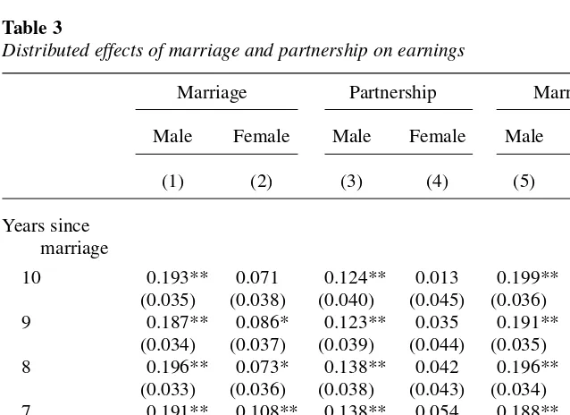
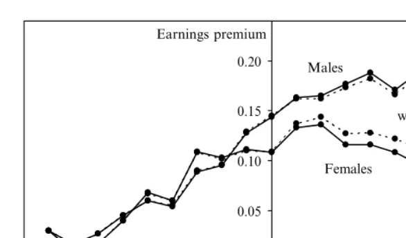
Column 1 of Table 3 presents the coefficients of the distributed marital status dummy variables estimated with fixed effects regressions with a ten-year maximum lag or lead. Observations outside the ten-year horizon were relatively few in number and were deleted. Figure 1 presents the coefficients graphically. The results are con-sistent with the notion that earnings do increase with maturation and that the effect is evident at least five years before marriage, and perhaps a few years earlier still. There is an increasing wage premium as the year of marriage approaches, and by the time of marriage the premium is 14 percent. The premium continues to rise for a few years after marriage, reaches a maximum of about 19 or 20 percent, and then levels off. Needless to say, these conclusions should be interpreted only as general tendencies found in a data set with a large number of observations.
The size of the effect is much greater than that suggested by a conventional fixed-effects specification with a single dummy variable for being married. However the discrepancy is accounted for by the change in the definition of the omitted marital
4. The cognitive ability score was a composite of the scaled scores of the arithmetic reasoning, word knowl-edge, and paragraph comprehension components of the Armed Services Vocational Aptitude Battery, with arithmetic reasoning being given double weight. The tests were administered to most of the NLSY respon-dents in 1980 as part of a project sponsored by the Department of Defense.
Table 1
Descriptive statistics
Male Female
Proportion married 0.50 0.53
Proportion in partnership 0.56 0.59
Mean earnings, married 14.94 11.23
Mean earnings, partnership 14.60 11.16
Mean earnings, single 11.46 10.33
Proportion with child age<6 0.31 0.29
Proportion with child 6<age<16 0.04 0.08
Table 2
Conventional estimates of the marriage and partnership premium
Marriage effects Partnership effects
Males Females Males Females
(1) (2) (3) (4)
OLS 0.151** −0.001 0.139** −0.001
(0.007) (0.006) (0.007) (0.007) Fixed effects 0.062** 0.026** 0.045 0.012
(0.008) (0.008) (0.007) (0.008)
n 20,187 14,781 20,009 14,475
Note: *, ** significant at the 5 percent, 1 percent levels.
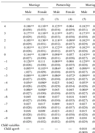
Table 3
Distributed effects of marriage and partnership on earnings
Marriage Partnership Marriage
Male Female Male Female Male Female
(1) (2) (3) (4) (5) (6)
Years since marriage
10 0.193** 0.071 0.124** 0.013 0.199** 0.092** (0.035) (0.038) (0.040) (0.045) (0.036) (0.038) 9 0.187** 0.086* 0.123** 0.035 0.191** 0.105**
(0.034) (0.037) (0.039) (0.044) (0.035) (0.037) 8 0.196** 0.073* 0.138** 0.042 0.196** 0.091**
(0.033) (0.036) (0.038) (0.043) (0.034) (0.036) 7 0.191** 0.108** 0.138** 0.054 0.188** 0.124**
(0.032) (0.035) (0.037) (0.042) (0.033) (0.05) 6 0.189** 0.096** 0.132** 0.050 0.185** 0.112**
(0.031) (0.033) (0.036) (0.041) (0.032) (0.034) 5 0.171** 0.108** 0.121** 0.071 0.166** 0.122**
Table 3 (continued)
Marriage Partnership Marriage
Male Female Male Female Male Female
(1) (2) (3) (4) (5) (6)
4 0.188** 0.116** 0.125** 0.064 0.182** 0.128** (0.030) (0.033) (0.034) (0.039) (0.031) (0.033) 3 0.177** 0.116** 0.119** 0.071 0.173** 0.127**
(0.029) (0.032) (0.033) (0.038) (0.030) (0.032) 2 0.165** 0.136** 0.118** 0.099* 0.162** 0.144**
(0.029) (0.031) (0.032) (0.037) (0.029) (0.031) 1 0.163** 0.133** 0.122** 0.078* 0.162** 0.137**
(0.028) (0.031) (0.032) (0.037) (0.028) (0.031) 0 0.144** 0.108** 0.098** 0.057 0.145** 0.109**
(0.027) (0.030) (0.031) (0.036) (0.027) (0.030) −1 0.128** 0.111 0.089** 0.068 0.129** 0.110**
(0.028) (0.030) (0.030) (0.035) (0.028) (0.030) −2 0.095** 0.103** 0.064* 0.067 0.096** 0.102**
(.027) (0.029) (0.030) (0.035) (0.027) (0.029) −3 0.089** 0.109** 0.060* 0.072* 0.090** 0.108**
(0.027) (0.029) (0.030) (0.035) (0.027) (0.029) −4 0.054* 0.060* 0.025 0.042 0.055* 0.060* (0.026) (0.029) (0.029) (0.034) (0.026) (0.029) −5 0.060* 0.068* 0.045 0.045 0.060* 0.067* (0.027) (0.030) (0.030) (0.035) (0.027) (0.030) −6 0.045 0.040 0.037 0.018 0.045 0.040
(0.027) (0.030) (0.030) (0.035) (0.027) (0.030) −7 0.027 0.017 0.009 0.015 0.027 0.017
(0.028) (0.030) (0.031) (0.037) (0.028) (0.030) −8 0.016 0.009 −0.023 −0.012 0.015 0.008
(0.028) (0.031) (0.031) (0.038) (0.028) (0.031) −9 0.030 0.030 0.001 0.059 0.030 0.030
(0.029) (0.032) (0.032) (0.039) (0.029) (0.032) Child variables
Child age<6 — — — — 0.010 −0.031**
(0.009) (0.009) Child 6<age<16 — — — — −0.040** −0.052**
(0.015) (0.014)
n 20,187 14,781 20,009 14,475 20,187 14,781
status category. In the distributed fixed effects model, the omitted category consists of those who remain single throughout the sample period. In a conventional specifica-tion, it also includes those who are single but who later marry. The latter, particularly those close to marriage, are already earning a premium, reducing the contrast. As a consequence, conventional studies may have tended to underestimate the marriage premium.
V. The Marriage Premium for Women
There has been relatively little theorizing about whether one should expect female earnings to be affected by marriage and it has mostly been limited to Becker-style suggestions that role specialization should adversely affect the earnings of married women by reducing investment incentives (Goldin and Polachek 1987). The reduction in incentives can have negative effects on work experience, tenure, and work intensity (Korenman and Neumark 1992), a precipitating factor being the pres-ence of children in the household (Hill 1979; Loury 1997). Employers may also dis-criminate against married women on the grounds that they are likely to have higher absence and turnover rates (Malkiel and Malkiel 1973).
Possibly the lack of attention to a female marriage effect is attributable to empiri-cal findings for, by contrast with males, there has been little sign of an effect even in simple cross-sectional studies. In those studies that disaggregate by ethnicity, a few report significant negative effects for white women and positive effects for black women (Carlson and Swartz 1988; Duncan 1996; Betts 2001). Significant negative effects for whites are reported by Loury (1997). Some studies find a significant positive effect for both white and black women (Oaxaca 1973; Blau and Beller 1988). However studies reporting a significant effect of any kind are in a small minority.
In view of the fact that most cross-sectional studies using OLS do not find an effect, there has been little incentive to pursue it with more sophisticated techniques and only a few have done so. Korenman and Neumark (1992) consider the possibility that mar-ital status, fertility, experience, and tenure may all be endogenous in a female wage equa-tion and use family characteristics and attitudinal variables to instrument for them. They conclude that marital status and fertility may be exogenous after all, and do not find a significant marital status effect in any of their specifications. Neumark and Korenman (1994) use sibling data to correct for unobserved heterogeneity as well as endogeneity. They find no significant effect in their fixed effects regressions for either white or black women assuming marital status to be exogenous. However, if marital status is treated as endogenous, its coefficient for white women is estimated at 0.46 to 0.53 and is sig-nificant at the 5 percent level. The authors do concede that these estimates appear to be implausibly high. The sample sizes were small (518 white and 248 black ob-servations). Kilbourne, England, and Beron (1994) find a significant positive effect for blacks, but no significant effect for whites, using panel data and fixed effects. Krashinsky (2004), using twins data and fixed effects, finds no significant effect.
the finding of a positive marriage premium for females. As in the case of males, there appears to be a maturation process that starts well in advance of marriage. Initially it appears to be very similar to that for males but it then attenuates a little in compari-son, reaching a premium of only 11 percent by the time of marriage and a maximum of 13 or 14 percent two years later. From that point it suffers a decline that ultimately reduces it to a premium of about 7 percent.
As in the case of males, a conventional specification of the wage equation leads to an underestimation of the marriage premium because the omitted category includes those who are soon to be married, and already earning a partial premium, as well as those who remain single.
VI. Partnership
Could the marriage effect on earnings really be a partnership effect? If this were the case, the rise in earnings before marriage could be a statistical artifact attributable to the distribution of premarital cohabitation and the growing probability of cohabitation as marriage approaches.
Both the conventional and distributed regressions were repeated replacing marriage with partnership, defined as living with an unrelated opposite sex individual in the household, with the results shown in Columns 3 and 4 of Table 2 and Columns 3 and 4 of Table 3. For both the conventional and distributed specifications, the pattern is similar to that for the marriage regressions. Earnings appear to rise as partnership approaches, and continue to rise after it has been established, in the same way as they do in the specification based on marriage. However, the coefficients are uniformly smaller in size, suggesting that marriage may in fact be the relevant relationship and that the regressions using partnership are subject to measurement error.
−0.05 0.00 0.05 0.10 0.15 0.20
−10 −8 −6 −4 −2 0 2 4 6 8 10
Males
Females
with child controls Earnings premium
Years married
Figure 1
VII. Children
The marriage earnings premium for males peaks about five years after marriage and then remains stable. By contrast, the premium for females peaks after only two years and then embarks on a steady decline. Several hypotheses could account for the asymmetry. An obvious one is that the establishment of the household eventually leads to domestic specialization in which the female may rationally be willing to accept a wage offer that undervalues her attributes if the job fits well with other responsibilities, especially looking after children. Another possibility is that the earnings of women raising families are adversely affected by an attenuation of labor force attachment. To investigate this, dummy variables for the presence of a child aged younger than six in the household, and for the presence of a child younger than 16 but not younger than six, were added to the specification for both males and females. The results are shown in Columns 5 and 6 of Table 3. In the case of males the change in specification has no systematic effect on the earnings profile. By con-trast, in the case of females the inclusion of the child variables does reduce the rate of decline. Abstracting from potential problems of endogeneity,5the results suggest that one or other of the suggested hypotheses might account for part of the decline in the marriage premium.
VIII. Conclusions
The present study, in characterizing the marriage premium as a dis-tributed fixed effect with origin some years before the time of marriage, appears to be compatible with most of the existing literature in the sense that it can account for previous findings.
It accounts for the finding of Korenman and Neumark (1991), Gray (1997) in his 1976–80 National Longitudinal Survey of Young Men sample, and Ginther and Zavodny (2001) that the marriage premium increases with years of marriage, and it accounts for the concavity of the effect.
It also confirms the premarriage effect found by Cornwell and Rupert (1997) and Krashinsky (2004). However it contradicts the finding of Cornwell and Rupert that the premium for to-be-married men is greater than that of married men and their conclu-sion that the marriage premium is an intercept shift that does not increase with years married.6The distributed fixed effect is consistent with Krashinsky’s finding that the wage growth of to-be-married men is similar to that of married men.
The present study is compatible with previous studies that have considered only an intercept shift, in that in a conventional specification there is an apparent premium of about 6 percent with fixed effects, but it implies that conventional studies substantially
5. One source of endogeneity arises from the possibility that couples may be more willing to embark upon a family, the greater their earnings. Another is the weak but well-established negative association between household income and number of children. The endogeneity issue is not pursued here for lack of suitable instruments.
underestimate the marriage premium because the omitted category merges those who are soon to be married with those who remain single.
The finding of a parallel, but smaller, distributed fixed effect for females contradicts the results of most previous studies in that only a few have found an effect of any kind. This can be explained by the fact that previous studies have looked for the potential premium in the form of a simple intercept shift. If the effect is distributed as suggested here, one would not anticipate a large difference between the earnings of married women, whose premium declines after a few years of marriage, and those of single women, who include those who are soon to be married and already earning a premium. The results appear to cast doubt on the specialization hypothesis because it is diffi-cult to reconcile it with the emergence of a premium five or more years before mar-riage. It also requires some ingenuity to explain how both sexes could simultaneously be specializing in the same direction.
References
Becker, Gary S. 1973. “A Theory of Marriage: Part One.” Journal of Political Economy
81(4):813–46.
———. 1974. “A Theory of Marriage: Part Two.” Journal of Political Economy
82(2):S11–S26.
———. 1981. A Treatise on the Family, Cambridge, Mass.: Harvard University Press Betts, Julian R. 2001. “The Impact of School Resources on Women’s Earnings and
Educational Attainment: Findings from the National Longitudinal Survey of Young Women.” Journal of Labor Economics19(3):635–57.
Blau, Francine D., and Andrea H. Beller. 1988. “Trends in Earnings Differentials by Gender.”
Industrial and Labor Relations Review41(4):513–29.
Carlson, Leonard A., and Caroline Swartz. 1988. “The Earnings of Women and Ethnic Minorities, 1959–1979.” Industrial and Labor Relations Review41(4):530–46.
Cornwell, Christopher, and Peter Rupert. 1997. “Unobservable Individual Effects, Marriage and the Earnings of Young Men.” Economic Inquiry, 35(2):285–94.
Duncan, Kevin C. 1996. “Gender Differences in the Effect of Education on the Slope of the Experience-Earnings Profiles.” American Journal of Economics and Sociology
55(4):457–71.
Ginther, Donna K., and Madeline Zavodny. 2001. “Is the Male Marriage Premium Due to Selection? The Effect of Shotgun Weddings on the Return to Marriage.” Journal of Population Economics14(2):313–28.
Goldin, Claudia, and Solomon Polachek. 1987. “Residual Differences by Sex: Perspectives on the Gender Gap in Earnings.” American Economic Review77(2):143–51.
Gray, Jeffrey S. 1997. “The Fall in Men’s Return to Marriage: Declining Productivity Effects or Changing Selection?” Journal of Human Resources32(3):481–504
Hill, Martha S. 1979. “The Wage Effects of Marital Status and Children.” Journal of Human Resources14(4):579–94.
Kilbourne, Barbara, Paula England, and Kurt Beron. 1994. “Effects of Individual, Occupation-al, and Industrial Characteristics on Earnings: Intersections of Race and Gender.”
Social Forces72(4):1149–76.
Korenman, Sanders, and David Neumark. 1991. “Does Marriage Really Make Men More Productive?” Journal of Human Resources26(2):282–307.
———. 1992. “Marriage, Motherhood, and Wages.” Journal of Human Resources
Krashinsky, Harry A. 2004. “Do Marital Status and Computer Usage Really Change the Wage Structure?” Journal of Human Resources29(3):774–91.
Loury, Linda D. 1997. “The Gender Earnings Gap among College-Educated Workers.”
Industrial and Labor Relations Review50(4):580–93.
Malkiel, Burton G., and Judith A. Malkiel. 1973. “Male-Female Pay Differentials in Professional Employment.” American Economic Review63(4):693–705. Neumark, David, and Sanders Korenman. 1994. “Sources of Bias in Women’s
Wage Equations.” Journal of Human Resources29(2):379–405.
Oaxaca, Ronald L. 1973. “Male-Female Wage Differentials in Urban Labor Markets.”