Studi Pengembangan Model Turbulen κ-ε untuk Sirkulasi Arus II: Aliran Turbulen Dua Dimensi pada Saluran Ekspansi

Studi Pengembangan Model Turbulen

κ

-

ε

untuk

Sirkulasi Arus II: Aliran Turbulen Dua Dimensi pada

Saluran Ekspansi

M. Syahril B. Kusuma, Rani A. Rahayu, Eka Oktarianto, Hadi Kardana & M. Cahyono

Kelompok Keahlian Teknik Sumber Daya Air Fakultas Teknik Sipil & Lingkungan ITB

Abstrak. Makalah ini menyajikan hasil studi pemodelan mengenai pola aliran turbulen 2 dimensi pada sebuah saluran yang mengalami ekspansi dengan memanfaatkan model depth averaged

κ

-ε. Model numerik dikembangkan berdasarkan metoda beda hingga, dimana untuk pemecahan persamaan hidrodinamik digunakan kombinasi metoda ekplisit Mac Cormack dan metoda pemisahan operator splitting. Sebagai tracer untuk melakukan visualisasi struktur aliran digunakan model transport kualitas air. Suku konveksi, difusi, dan reaksi diselesaikan dengan skema QUICKEST, Central Scheme, dan Euler Scheme. Hasil yang dicapai model dalam mensimulasikan pola arus untuk kasus saluran lurus dan ekspansi menunjukan tingkat kesesuaian yang cukup baik dengan hasil pengukuran di Laboratorium. Dibandingkan dengan model non turbulen, hasil model menunjukkan peningkatan akurasi yang signifikan dalam hal besar kecepatan arus, pola arus dan sebaran konstituent kualitas air, terutama pada zona resirkulasi. Model dapat mensimulasikan pola sirkulasi arus dan terbentuknya vorteks pada zona sirkulasi. Namun demikian, untuk aliran dengan bilangan Reynold cukup rendah, osilasi dan ketidakstabilan numerik masih menjadi kendala.

Kata kunci: aliran turbulen 2 dimensi; depth averaged kappa-epsilon model; pola arus; saluran ekspansi.

Abstract. This paper present the results of modeling study of two dimensions turbulent flow in an expansion canal by using depth averaged

κ

-ε model. The numerical model was developed using finite difference method where hydrodynamic equation was solved by the combination of Mac Cormack and splitting methods. Water quality distribution is used as a tracer to visualize the flow structure. QUICKEST, Central, and Euler Scheme are used to find convection, diffusion, and reaction term solution. Model results have shown good agreement with those found by laboratory measurement and better assessment compared to those found by non turbulent model. In general, the result had shown better assessment on flow structure, velocity field, turbulent/vortex bursting and water quality distribution compared to those resulted by non turbulent model. But for small Reynolds number turbulent flow, where more densed grid and high courant number is needed, the model become oscillating and unstable.

Makalah diterima redaksi tanggal 13 November 2006, revisi diterima tanggal 26 April 2007, diterbitkan tanggal 26 April 2007.

Keywords:depth averaged kappa-epsilon model; expansion canal; flow pattern; two D turbulent flow.

1

Pendahuluan

Pada perencanaan jaringan tata air, masalah ekspansi (pelebaran) saluran seringkali tidak dapat dihindari sebagai akibat adanya kebutuhan penyesuaian dimensi saluran terhadap perubahan debit, persilangan bangunan dengan saluran, kondisi topografi, dll.

Penelitian mengenai struktur aliran pada saluran ekspansi telah banyak dilakukan, namun untuk aliran dengan fluida cair, kebanyakan dari penelitian tersebut bersifat eksperimental dan fokus pada masalah gerusan dan aliran di luar daerah sirkulasi, sementara itu untuk struktur aliran pada zona resirkulasi banyak dilakukan terutama untuk aliran dengan fluida udara. Uraian pada paragraf di bawah ini membahas rangkuman dari beberapa hasil penelitian mengenai struktur aliran turbulen akibat penurunan dasar saluran yang sebagian besar berlaku untuk kasus fluida udara.

Pada batas awal sebuah saluran ekspansi, massa fluida akan lepas landas dari dinding membentuk free mixing layer di bagian hilir dan akan menyentuh

dinding kembali pada titik yang disebut reattachment point setelah menempuh

jarak tertentu yang disebut reattachment length [1]. Pada saluran yang

mengalami ekspansi sebesar H, posisi reattachment point berfluktuasi pada

daerah sepanjang 2 H dan panjang reattachment length bervariasi antara 4-10 H,

bergantung pada turbulensi aliran pada bagian hulu ekspansi [2]. Sepanjang jarak reattachment length tersebut aliran mengalami gradient tekanan positif

dan tidak stabil karena membentuk zona resirkulasi pada daerah sekitar dinding. Pada zona ini, arah aliran berlawanan dengan arah aliran utama. Kondisi ini mengakibatkan aliran tidak stabil dan bersifat turbulen [3-5]. Pada zona tersebutlah struktur coherent turbulen akan terbentuk secara periodik melalui

apa yang disebut fenomena bursting [2, 3, 5]. Pada zona resirkulasi kecepatan

fluktuasi menjadi besar dan dapat melebihi kecepatan rata-rata aliran. Pada titik

reattachment akan terjadi pembelahan vorteks yang berlawanan arah, satu

vorteks menuju zona resirkulasi dan satu vorteks mengalir menuju hilir [2, 6]. Pada zona resirkulasi, vorteks mempunyai kemampuan untuk menstimulir pembentukan vorteks yang berlawanan arah sebagai konsekuensi dari kekekalan massa [2]. Pada prinsipnya, proses yang sama dengan karakteristik yang berbeda akan dialami oleh sebuah massa fluida cair bila dialirkan melalui saluran tersebut di atas. Perbedaan karakteristik ini terutama diakibatkan adanya pengaruh gravitasi pada fluida cair. Perbedaan yang dapat dengan mudah di identifikasi antara lain adalah bilangan Reynold karakteristik turbulen, panjang

reattachment lenght, bursting karakteristik dan ketebalan lapisan mixing layer

[7-10].

Metoda penyelesaian masalah terbulen tersebut diatas telah banyak dikembangkan, antara lain adalah metoda Zero equation model, One equation

model, Reynolds stress model dan Two equation κ-ε model. Namun demikian,

karena tingkat akurasi yang diberikan cukup baik, metoda two equation κ-ε

model lebih banyak dikembangkan, seperti yang akan disajikan/dibahas pada

makalah ini.

2

Persamaan Pengatur

Persamaan pengatur aliran ini diturunkan berdasarkan persamaan Navier-Stokes untuk aliran turbulen 2 dimensi tak mampu mampat dalam bentuk

depth-averaged velocity. Beberapa anggapan yang dipakai dalam melakukan

penurunan persamaan pengatur tersebut adalah sbb: 1. Fluida tak mampu mampat (incompressible)

2. Kecepatan aliran yang ditinjau adalah kecepatan rata-rata 3. Aliran adalah dua dimensi (arah –x dan arah-y)

4. Kemiringan dasar saluran relatif kecil (sin~tangen~kemiringan saluran) 5. Distribusi tekanan fluida bersifat hidrostatis (viscous stress diabaikan)

6. Pengaruh gaya putaran bumi (efek coriolis) diabaikan

7. Konstituent tercampur merata (well mixed).

2.1

Persamaan Kontinuitas & Momentum

Dengan menerapkan prinsip dekomposisi Reynold terhadap besaran aliran turbulen, persamaan rata-rata kontinyuitas dan momentum untuk aliran tiga dimensi dapat dituliskan secara berturutan dalam bentuk sbb.:

i i u 0 x ∂ ₌ ∂ (1) j ' ' i i i j i i j i j j i u u _u u _g 1 p 1 u _u t x x x x x uj ⎡ ⎛ ∂ ⎞ ⎤ ∂ ₊ ∂ _{= −} ∂ _{+ ∂ ⎢μ⎜}∂ _{+ ⎟− ρ ⎥} ⎜ ⎟ ∂ ∂ ρ ∂ ρ ∂ ⎢_{⎣ ⎝}∂ ∂ _⎠ ⎥_⎦ (2)

Integrasi persamaan (1) dan (2) terhadap kedalaman dengan menggunakan metode “Leibnitz Rule” akan memberikan persamaan rata-rata kontinyuitas dan momentum dalam bentuk Depth-Averaged Velocity untuk aliran 2 dimensi tak

Persamaan Kontinuitas

(

UH

)

( )

VH H 0 t x y ∂ ∂ ⎡ ⎤ ⎡ ⎤ ∂ ⎡ _{⎤ + +} ⎢ ⎥ ⎢ ⎥ ⎢_∂ ⎥ _{∂ ∂} ⎣ _{⎦ ⎣ ⎦ ⎣ ⎦}= (3)

Persamaan Momentum

Arah x

( )

2

(

)

(

)

( )

xy xx 2 1 1 1 1 0x bx Sx h hU gh hUV h hU ghS t x 2 y ρ ρ x ρ y ρ ∂ τ ∂ ₊ ∂ ⎛ ₊ ⎞₊∂ _{= − τ +} ∂ τ _{+ +} ⎜ ⎟ ∂ ∂ _{⎝ ⎠} ∂ ∂ ∂ τ (4) Arah y

( )

2

(

)

( )

( )

xy yy 2 1 1 1 1 0y by Sy h h hV gh hUV hV ghS t y 2 x ρ ρ y ρ y ρ ∂ τ ∂ τ ∂ ₊ ∂ ⎛ ₊ ⎞₊∂ _{= − τ + + +} ⎜ ⎟ ∂ ∂ _{⎝ ⎠} ∂ ∂ ∂ τ (5) dimana h h 1 1 U udz V vdz h h η η − − = = + η

∫

+ η

∫

' ' xx

u

2

u u

x

∂

τ = μ

− ρ

∂

' ' yy v 2 v y ∂ τ = μ − ρ ∂ v ' ' xy u v u v y x ⎛∂ ∂ ⎞ τ = μ_⎜⎜ + _⎟⎟− ρ ∂ ∂ ⎝ ⎠ bx

τ dan τ_sx masing-masing merupakan tegangan dasar saluran dan tegangan

permukaan air, sedangkan dan masing-masing merupakan kemiringan

enerji pada arah x dan y.

x

0

S

S_0y

2.2

Persamaan Model Turbulen

κ

-

ε

Persamaan (2) sangat kompleks dan untuk penyelesaiannya membutuhkan

Closure Problem dari suku “Reynold Stress” yang dalam hal ini dapat didekati

j i i j t ij j i ( U ) ( U ) _{2 ˆ} ˆ u u kh x x 3 ∂ ∂ ′ ′ − = ν + − δ ∂ ∂

⎡

⎤

⎢

⎥

⎣

⎦

(6) dimana ij δ = delta Kronecker ij i j, 1 i j, 0 = δ = ⎧ δ ⎨ _{≠ δ =} ⎩ (7)

Dari analisis dimensional, didapatkan bahwa besaran eddy viscosity (νt)

sebanding dengan karakteristik skala kecepatan (v) dan skala panjang ( ), yaitu

νt≈

v

l

.

l

Model turbulen κ-ε dikembangkan untuk menyelesaikan persamaan Reynold Stress dengan menggunakan 2 persamaan tambahan yaitu Turbulence

Kinetic-Energy Equation dan Turbulence Energy Dissipation Rate Equation. Persamaan

Enerji Kinetik Turbulen tersebut dapat dituliskan sbb.: j j i j j i j i iii i _ii u p ' k k 1 u u ' u ' u ' u ' u ' t x x 2 ⎡ ⎤ j i x ∂ ⎛ ⎞ ∂ ∂ ∂ + = − ⎢ _⎜ + _⎟⎥− ∂ ∂ ∂ _{⎢⎣ ⎝} ρ _⎠⎥⎦ ∂ 14243 14243 1444442444443 i j j j i j i i j v iv u ' u ' u ' u ' u ' u ' x x x x x ⎡ _{⎛∂ ∂ ⎞}⎤ _{∂ ⎛∂ ∂ ⎞} ∂ ⎢ ⎥ + ν ⎜_⎜ + ⎟_⎟ − ν ⎜_⎜ + ∂ ⎢_{⎣ ⎝}∂ ∂ _⎠⎥_⎦ ∂ _⎝∂ ∂ _⎠ j i i x ⎟⎟ 144424443 14444244443 (8)

Pada persamaan (8) tersebut, suku (i), (ii), (iii), (iv) dan (v) adalah suku-suku yang menunjukkan laju perubahan energi turbulen, convective diffusion energi

turbulen, produksi energi turbulen, kerja turbulen stresses dan turbulent viscous

dissipation. Bila ν diasumsikan konstan maka persamaan (8) menjadi:

j i j j j i p ' k k 1 u u ' u ' u ' t x x 2 ⎡ _{⎛ ⎞}⎤ ∂ ₊ ∂ _{= −} ∂ ₊ ⎢ _{⎜ ⎟}⎥ ∂ ∂ ∂ ⎢_⎣ ⎝ ρ⎠⎥_⎦ 2 j i i i j i j j j u k u ' u ' u ' u ' x x x x x ∂ j ∂ ∂ ∂ − + ν − ν ∂ ∂ ∂ ∂ ∂ (9)

Launder & Spalding [11] menuliskan persamaan (9) diatas dalam bentuk: t j j j k j k x ∂ k k u t x x ⎛ν ⎞ ∂ ∂ ∂ + = − ⎜_⎜ ⎟_⎟ ∂ ∂ ∂ _⎝σ ∂ _⎠ 3 / 2 j i i t D j i j u u u k v C x x x ⎛∂ ∂ ⎞∂ + ⎜_⎜ + ⎟_⎟ − ∂ ∂ ∂ ⎝ ⎠ l (10)

Sementara itu, persamaan Turbulence Energy Dissipation Rate (ε) dapat dituliskan sbb.: i i j k j j j k k i i _ii u ' u ' u ' u ' u u 2 t x x x x x x ⎛∂ ∂ ∂ ∂ ⎞ ∂ε₊ ∂ε _{= − ν∂ ⎜ + ⎟} ⎜ ⎟ ∂ ∂ ∂ _⎝∂ ∂ ∂ ∂ _⎠ 14243 1444444 k j 24444443 2 i i i i j i j k k j k k iv iii u ' u ' u ' u ' u 2 u ' 2 x x x x x x ∂ ⎛ ∂ ⎞ ∂ ∂ ∂ − ν ⎜_⎜ ⎟_⎟− ν ∂ ∂ _⎝ ∂ _⎠ ∂ ∂ ∂ 144424443 144424443

( )

2 2 i i j j k j i k k vii vi v u ' p ' u ' 2 u ' x x x x x x ⎛ ∂ ⎞ ∂ ν ∂ ⎛∂ ∂ ⎞ − ⎜_⎜ν_{∂ ∂} ⎟_⎟ −_∂ ε −_{ρ ∂} ⎜_{∂ ∂} ⎟ ⎝ ⎠ ⎝ ⎠ _{14243 144424443} 1442443 2 j j viii x x ∂ ε + ν ∂ ∂ 14243 (11)

dimana suku (i), (ii)+(iii), (iv), (v), (vi)+(vii)+(viii) adalah suku-suku yang menunjukkan laju perubahan ε, transport energi kinetis oleh interaksi dengan gerakan rata-rata (generation of ε by mean flow), transfer energi kinetis oleh

efek kecepatan (generation of ε by self stretching of vortex tube), viscous

destruction dan difusi. Persamaan (11) disederhanakan oleh Launder and

Spalding [11] menjadi sebagai berikut:

k C P k C x x x u t _j t j j j 2 2 1 ε ε ε σ ν ε ε ε ε ε − + ⎟ ⎟ ⎠ ⎞ ⎜ ⎜ ⎝ ⎛ ∂ ∂ ∂ ∂ − = ∂ ∂ + ∂ ∂ ₍₁₂₎ dimana: j i t j i u u P v x x x ⎛ ∂ ⎞ _i j u ∂ ∂ = ⎜_⎜ + ⎟_⎟ ∂ ∂ ∂ ⎝ ⎠ (13)

Persamaan tersebut diatas hanya dapat digunakan untuk menyelesaikan

closure-problem dari persamaan reynolds stress dalam bentuk depth averaged setelah

dimodifikasi dalam bentuk depth integrated. Dalam hal ini, Chapman and Kuo

[12] telah memodifikasi model Rastogi and Rodi [13] dalam bentuk persamaan yang lebih konsisten dengan persamaan kontinuitas depth averaged dan

persamaan momentum depth averaged sehingga diperoleh hubungan

depth-integrated Reynolds stresses dengan depth integrated strain rates sebagai

berikut: b b h z j i i j ij j i z (v U ) (v U ) 1 _{2 ˆ} ˆ u u dz kh h x x + _{⎡∂ ∂ ⎤} ′ ′ − = ν ⎢ + ⎥− ∂ ∂ ⎢ ⎥ ⎣ ⎦

∫

₃ δ (14)

dimana

δ

_ij adalah delta kronecker dan

ν

ˆ

t adalah Viskositas Turbulen untuk

depth averaged yang dapat dituliskan sebagai berikut:

ˆ

ˆ

ˆ

2 t μ

k

ν

= C

ε

(15)

Pemodelan pada makalah ini menggunakan model Turbulen κ-ε yang diperoleh dari pendekatan Chapman and Kuo [12] tersebut di atas sehingga diperoleh persamaan energi kinetis turbulen dan laju disipasi energi turbulen yang berlaku untuk persamaan depth averaged sbb.:

• Persamaan Κ = ∂ ∂ + ∂ ∂ + ∂ ∂ y k h x k h t k hˆ) ( U ˆ) ( Vˆ) ( _{p p h} y k h y x k h x _k h k t k t

ε

σ

ν

σ

ν

ˆ ( ˆ) ˆ ( ˆ) _ˆ − + + ⎥ ⎥ ⎦ ⎤ ⎢ ⎢ ⎣ ⎡ ∂ ∂ ∂ ∂ + ⎥ ⎥ ⎦ ⎤ ⎢ ⎢ ⎣ ⎡ ∂ ∂ ∂ ∂ ₍₁₆₎ • Persamaan ε ⎥ ⎦ ⎤ ⎢ ⎣ ⎡ ∂ ∂ ∂ ∂ = ∂ ∂ + ∂ ∂ + ∂ ∂ x h y y h x h t hˆ) ( U ˆ) ( V ˆ) ˆ_t ( ˆ) ( ε σ ν ε ε ε ε _ε ε

ε

ε

ε

σ

ν

p h C p C k y h y h t + − + ⎥ ⎦ ⎤ ⎢ ⎣ ⎡ ∂ ∂ ∂ ∂ + ˆ ( ˆ) _ˆˆ( _{1 2}ˆ ) (17) dimana:

( )

( )

( )

( )

⎪⎭ ⎪ ⎬ ⎫ ⎪⎩ ⎪ ⎨ ⎧ ⎥ ⎦ ⎤ ⎢ ⎣ ⎡ ∂ ∂ + ∂ ∂ + ⎥ ⎦ ⎤ ⎢ ⎣ ⎡ ∂ ∂ + ⎥⎦ ⎤ ⎢⎣ ⎡ ∂ ∂ = Ρ 2 2 2 V h h U V h 2 h U 2 ˆ x y y x h t h ν ₍₁₈₎ U q , C hD , 2 2 5/2 1/2 4 4 / 5 2 / 1 2 3 2 V q g C C q C g k = Ρ = = + Ρ _ε μ (19)

dimana besaran koefisien-koefisien pada persamaan tersebut adalah : Cμ= 0.09,

C1= 1.44, C2 = 1.92, σk = 1.0, σε = 1.3 dan D = 0.075

Secara lengkap persamaan hidrodinamik dan κ-ε diatas dapat dituliskan kembali dalam bentuk sebagai berikut:

$ $ $ t 2 t 2 t k t 0 HU 2 2 Hk H UH VH x 3 HU U H UVH HU HV y x HV UVH V H t x _ˆ y _ˆ x _ˆ ˆ Hk UH k H V k (Hk) x ˆ ˆ UH H V H ˆ (H )ˆ x ε ⎡ ⎤ ⎢ _∂ ⎥ ⎢ ν − ⎥ ⎡ ⎤ ⎡ ⎤ ⎡ ⎤ ⎢ ∂ ⎥ ⎢ ⎥ ⎢ ⎥ ⎢ ⎥ ⎢ _{⎛∂ ∂ ⎞}⎥ ⎢ ⎥ ⎢ ⎥ ⎢ ⎥ ⎢ν _⎜ + _⎟⎥ ∂_{⎢ ⎥+}∂ _{⎢ ⎥+}∂_{⎢ ⎥=} ∂_{⎢ ⎝ ∂ ∂ ⎠⎥} ⎢ ⎥ ⎢ ⎥ ⎢ ⎥ ⎢ ⎥ ∂ ∂ ∂ ∂ ν ⎢ ⎥ ⎢ ⎥ ⎢ ⎥ ⎢ ∂ ⎢ ⎥ ⎢ ⎥ ⎢ ⎥ ⎢ _{σ ∂} ε ε ε ⎢ ⎥ ⎢ ⎥ ⎢ ⎥ ⎣ ⎦ ⎣ ⎦ ⎢ ⎣ ⎦ ⎢ ν ∂ ε ⎢ σ ∂ ⎢⎣ ⎦ $ $ $ $ [ ] ( ) ( ) 2 2 a x ox 2 2 2 a y oy 2 2 t t t t k t 0 C* W W gU U V gHS C C* W W gV U V gHS C h U h V 0 _{2 2} x y ˆ HU HV y x h HV 2 2 Hk y 3 y _ˆ ˆ (Hk) y ˆ (H )ˆ y ε ⎡ _{+ ρ} ⎤ ⎢ − + ⎥ ρ ⎢ ⎥ ⎣ ⎦ ⎡ + ρ ⎤ ⎢ − + ⎥ ρ ⎢ ⎥ ⎣ ⎦ ⎡∂ ⎤ ⎡∂ ⎤ ⎡ ⎤ _{⎢ ⎥ + ⎢} ⎢ _{⎛∂ ∂ ⎞}⎥ _{ν ⎢ ∂ ⎥ ⎢ ∂} ⎣ ⎦ ⎣ ⎢_{ν⎜ + ⎟}⎥ ⎢ ⎝ ∂ ∂ ⎠⎥ ⎢ ⎥ ∂ ⎢ _{ν −} ⎥ ∂ ⎢ _∂ ⎥ + _{⎢ ⎥}+ ∂ ⎢ ⎥ ⎥ ν ∂ ⎢ ⎥ ⎥ _{σ ∂} ⎢ ⎥ ⎥ ⎢ ⎥ ⎥ _⎢ ν ∂ ε _⎥ ⎥ σ ∂ ⎥ ⎢_⎣ ⎥_⎦ ( ) ( )

(

)

( ) ( ) ( ) ( ) 2 2 3 2 2 2 2 2 t 1 ₂ 2 h U h V y x g _ˆ U V h C h U h V 2 2 x y ˆ ˆ ˆ C C ˆ h k h U h V y x ⎡ ⎧ ⎫⎤ ⎢ ⎪ _⎥⎪⎥ ⎢ ⎪_{⎪ ⎥⎦}⎪⎥ ⎢ _{⎨ ⎬}⎥ ⎢ _{⎪ ⎡∂ ∂ ⎤ ⎪}⎥ ⎢ _{⎪+⎢ + ⎥ ⎪}⎥ ⎢ _{⎪⎩ ⎢⎣} ∂ ∂ _{⎥⎦ ⎪⎭}⎥ ⎢ ⎥ ⎢ _{⎧ ⎫} ⎥ ⎢+⎨ + ⎬− ε ⎥ ⎢ ⎩ ⎭ ⎥ ⎣ ⎦ ⎛ ⎧ _{⎡∂ ⎤ ⎡∂ ⎤}⎫ ⎞ ⎜ ⎪ ⎢ ⎥ + ⎢ ⎥⎪ ⎟ ⎜ ν ⎪ ⎢ ∂ ⎥ ⎢ ∂ ⎥⎪ ⎟ ε_⎜ ⎪ ⎣ ⎦ ⎣ ⎦ ⎪_{− ε ⎟} ⎨ ⎬ ⎜ _{⎪ ⎡∂ ∂ ⎤ ⎪} ⎟ ⎜ _{⎪+⎢ + ⎥ ⎪} ⎟ ⎜ ⎟ ⎜ ⎪⎩ ⎢⎣ ∂ ∂ ⎥⎦ ⎪⎭ ⎝ ⎠ h ⎪

(

)

4 1/ 2 5 / 4 2 2 2 1/2 5/2 C C g U V hD C μ ⎡ ⎤ ⎢ ⎥ ⎢ ⎥ ⎢ ⎥ ⎢ ⎥ ⎢ ⎥ ⎢ ⎥ ⎢ ⎥ ⎢ ⎥ ⎢ ⎥ ⎢ ⎥ ⎢ ⎥ ⎢ ⎥ ⎢ ⎥ ⎢ ⎥ ⎢ ⎥ ⎢ ⎥ ⎢ ⎥ ⎢ ⎥ ⎢ ⎥ ⎢ ⎥ ⎢ ⎥ ⎡ ⎤ ⎢ ⎥ ⎢ ⎥ ⎢ ⎥ ⎢ ⎥ ⎢ ⎥ ⎢ ⎥ ⎢ ⎥ ⎢ ⎥ ⎢ ⎥ ⎢ ⎥ ⎢ ⎥ ⎢ ⎥ ⎢ ⎟⎥ ⎢ ⎥ ⎢ ⎥ ⎢ ⎥ ⎢ _{⎧ ⎫} ⎥ ⎢ ⎥ ⎢ _⎪⎪ + _⎪⎪ ⎥ ⎢ ⎥ ⎢_{+ ⎨ ⎬} ⎥ ⎢ ⎥ ⎢ _{⎪ ⎪} ⎥ ⎢ ⎥ ⎢ _{⎪ ⎪} ⎥ ⎢ ⎩ ⎭ ⎥ ⎢⎣ ⎦⎥ ⎢⎣ ⎦⎥ (20)

2.3

Persamaan Transport Konstituent Kualitas Air

Persamaan transport konveksi-difusi, yang penurunannya didasarkan pada penggunaan hukum kekekalan massa di ruang tilik, dapat dituliskan sbb.:

( )

(

U

)

(

V

)

Dx D t x x x x x ⎛ ⎞ ∂ _{Φ +} ∂ _{Φ +} ∂ _{Φ =} ∂ ⎛ ∂Φ⎞₊ ∂ ∂ ⎜ ⎜ ⎟ ∂ ∂ ∂ ∂ ⎝ ∂ ⎠ ∂ ⎝ y ∂y⎠ Φ ⎟ (21)

2.4

Syarat Batas

Pada kondisi batas perairan diterapkan syarat batas Inward Difference,

sedangkan pada dinding dianggap kecepatan aliran sama dengan nol.

3

Penyelesaian Numerik

Metoda penyelsaian numerik dari persamaan yang digunakan adalah sbb.:

1. Persamaan hidrodinamik diselesaikan dengan Skema Mac

Cormack-Splitting.

2. Persamaan κ-ε diselesaikan dengan Skema QUICKEST pada suku

konveksi, Skema Central Difference pada suku difusi, dan Skema Euler

pada suku reaksi.

3. Persamaan kualitas air/material transport (salinitas) dengan skema

3.1

Penyelesaian Numerik Hidrodinamika dengan Teknik Mac

Cormack-

Splitting

Secara lengkap skema splitting untuk persamaan Hidrodinamik adalah:

(

) (

)

n 2 n

x y xx yy s s yy xx y x

F + =⎡_⎣ L L L L L • L L L L L ⎤_⎦F

Suku Lx, Ly, Lxx, Lyy dan Ls diselesaikan dengan metode Mac Cormack sbb.:

1. Penyelesaian numerik persamaan diferensial orde satu

L

x

Predictor $ n n * n n n 2 2 n i, j i, j i, j _{i, j i 1, j} i, j i 1, j n i, j UH UH H H 0 0 t t UH UH U H U H gH H z H z x x VH VH UVH UVH 0 0 0 t 2 Hk x 3 0 − − ⎧_{⎡ ⎤ ⎡ ⎤} ⎫ _{⎧ ⎫} ⎡ ⎤ ⎡ ⎤ _{⎪ ⎪ ⎪}⎡ ⎤ ⎡ ⎤ _⎪ ⎢ ⎥ ⎢ ⎥ Δ ⎪ ⎪ Δ ⎪ ⎢ ⎥ ₌⎢ ⎥ _{− ⎨ − ⎬− ⎨}⎢ ₊ ⎥ ₋⎢ ₊ ⎥ ⎢ ⎥ ⎢ ⎥ ⎢ ⎥ ⎢ ⎥ _{Δ Δ} ⎢ ⎥ ⎢ ⎥ ⎪⎢ ⎥ ⎢ ⎥ ⎪ ⎪ ⎢ ⎥ ⎢ ⎥ ⎢ ⎥ ⎢ ⎥ ⎣ ⎦ ⎣ ⎦ ⎣ ⎦ ⎣ ⎦ ⎪ ⎬ ⎪ ⎪ ⎪ ⎣ ⎦ ⎣ ⎦ ⎪ ⎪ ⎩ ⎭ ⎩ ⎭ ⎡ ⎤ ⎢ ⎥ Δ _{⎢ ⎥} + − − ⎢ ⎥ Δ ⎢ ⎥ ⎣ ⎦ $ n i 1, j 0 2 Hk 3 0 − ⎧ _{⎡ ⎤} ⎫ ⎪ _{⎢ ⎥} ⎪ ⎪ _{⎢− ⎥} ⎪ ⎨ _{⎢ ⎥} ⎬ ⎪ _{⎢ ⎥} ⎪ ⎪ _{⎣ ⎦} ⎪ ⎩ ⎭ (22) Corrector $ * * ** * * * 2 2 n i, j i, j i, j _{i 1, j i, j} i 1, j i, j i 1, UH UH H H 0 0 t t UH UH U H U H gH H z H z x x VH VH UVH UVH 0 0 0 t 2 Hk x 3 0 + + + ⎧_{⎡ ⎤ ⎡ ⎤} ⎫ _{⎧ ⎫} ⎡ ⎤ ⎡ ⎤ _{⎪ ⎪ ⎪}⎡ ⎤ ⎡ ⎤ _⎪ ⎢ ⎥ ⎢ ⎥ Δ ⎪ ⎪ Δ ⎪ ⎢ ⎥ ₌⎢ ⎥ _{− − −} ⎢ ₊ ⎥ ₋⎢ ₊ ⎥ ⎨⎢ ⎥ ⎢ ⎥ ⎬ ⎨ ⎢ ⎥ ⎢ ⎥ _{Δ ⎪ ⎪ Δ ⎪}⎢ ⎥ ⎢ ⎥ ⎢ ⎥ ⎢ ⎥ ⎢ ⎥ ⎢ ⎥ ⎢ ⎥ ⎢ ⎥ ⎣ ⎦ ⎣ ⎦ ⎣ ⎦ ⎣ ⎦ ⎪ ⎬ ⎪ ⎪ ⎪ ⎣ ⎦ ⎣ ⎦ ⎪ ⎪ ⎩ ⎭ ⎩ ⎭ ⎡ ⎤ ⎢ ⎥ Δ ⎢ ⎥ + − ⎢ ⎥ Δ ⎢ ⎥ ⎣ ⎦ $ * * j i, j 0 2 Hk 3 0 ⎧ _{⎡ ⎤} ⎫ ⎪ _{⎢ ⎥} ⎪ ⎪ _{− −⎢ ⎥} ⎪ ⎨ _{⎢ ⎥} ⎬ ⎪ _{⎢ ⎥} ⎪ ⎪ _{⎣ ⎦} ⎪ ⎩ ⎭ (23) n+1 n 1 * ** i, j i, j i, j H H H 1 UH UH UH 2 VH VH VH + _{⎧ ⎫} ⎡ ⎤ _⎪⎡ ⎤ ⎡ ⎤ _⎪ ⎪ ⎪ ⎢ ⎥ _{= ⎨}⎢ ⎥ ₊⎢ ⎥ ⎢ ⎥ _⎪⎢ ⎥ ⎢ ⎥ _⎪ ⎢ ⎥ ⎢ ⎥ ⎢ ⎥ ⎣ ⎦ _⎪⎩⎣ ⎦ ⎣ ⎦ _⎪⎭ ⎬ (24)

2. Penyelesaian numerik persamaan diferensial orde satu

L

y Predictor $ n n * n n n n i, j 2 2 i, j i, j _{i, j i 1, j} i, j i 1, j i H H UH UH 0 0 t t UH UH UVH UVH gH 0 0 y y VH VH _{V H V H} z H z H 0 t 0 y 2_Hk 3 − − ⎧_{⎡ ⎤ ⎡ ⎤} ⎫ ⎧ ⎫ ⎡ ⎤ ⎡ ⎤ _{⎪ ⎪ ⎪}⎡ ⎤ ⎡ ⎤ _⎪ ⎢ ⎥ ⎢ ⎥ Δ ⎪ ⎪ Δ ⎪ ⎢ ⎥ ₌⎢ ⎥ _{− − −} ⎢ ⎥ ₋⎢ ⎥ ⎨⎢ ⎥ ⎢ ⎥ ⎬ ⎨ ⎢ ⎥ ⎢ ⎥ _{Δ ⎪ ⎪ Δ ⎪}⎢ ⎥ ⎢ ⎥ ⎢ ⎥ ⎢ ⎥ ⎢ ⎥ ⎢ ⎥ ⎢ + ⎥ ⎢ + ⎥ ⎣ ⎦ ⎣ ⎦ ⎣ ⎦ ⎣ ⎦ ⎣ ⎦ ⎣ ⎦ ⎪ ⎬ ⎪ ⎪ ⎪ ⎪ ⎪ ⎩ ⎭ ⎩ ⎭ ⎡ ⎤ ⎢ ⎥ ⎢ ⎥ Δ + _{⎢ ⎥} Δ _{⎢ ⎥} ⎢− ⎥ ⎢ ⎥ ⎣ ⎦ $ n n , j i 1, j 0 0 2_Hk 3 − ⎧ _{⎡ ⎤} ⎫ ⎪ _{⎢ ⎥} ⎪ ⎪ _{⎢ ⎥} ⎪ ⎪ ₋ ⎪ ⎨ ⎢ ⎥ ⎬ ⎪ ⎢ ⎥ ⎪ ⎪ ⎢_⎢− ⎥_⎥ ⎪ ⎣ ⎦ ⎪ ⎪ ⎩ ⎭ (25) Corrector $ * * ** * * * n i, j 2 2 i, j i, j _{i 1, j i, j} i 1, j i, j H H UH UH 0 0 t t UH UH UVH UVH gH 0 0 y y VH VH _{V H V H} z H z H 0 t 0 y 2_Hk 3 + + ⎧_{⎡ ⎤ ⎡ ⎤} ⎫ ⎧ ⎫ ⎡ ⎤ ⎡ ⎤ _{⎪ ⎪ ⎪}⎡ ⎤ ⎡ ⎤ _⎪ ⎢ ⎥ ⎢ ⎥ Δ ⎪ ⎪ Δ ⎪ ⎢ ⎥ ₌⎢ ⎥ _{− − −} ⎢ ⎥ ₋⎢ ⎥ ⎨⎢ ⎥ ⎢ ⎥ ⎬ ⎨ ⎢ ⎥ ⎢ ⎥ _{Δ ⎪ ⎪ Δ ⎪}⎢ ⎥ ⎢ ⎥ ⎢ ⎥ ⎢ ⎥ ⎢ ⎥ ⎢ ⎥ ⎢ + ⎥ ⎢ + ⎥ ⎣ ⎦ ⎣ ⎦ _{⎣ ⎦ ⎣ ⎦} ⎣ ⎦ ⎣ ⎦ ⎪ ⎬ ⎪ ⎪ ⎪ ⎪ ⎪ ⎩ ⎭ ⎩ ⎭ ⎡ ⎤ ⎢ ⎥ ⎢ ⎥ Δ + _{⎢ ⎥} Δ _{⎢ ⎥} ⎢− ⎥ ⎢ ⎥ ⎣ ⎦ $ * * i 1, j i, j 0 0 2_Hk 3 + ⎧ _{⎡ ⎤} ⎫ ⎪ _{⎢ ⎥} ⎪ ⎪ _{⎢ ⎥} ⎪ ⎪ ₋ ⎪ ⎨ ⎢ ⎥ ⎬ ⎪ ⎢ ⎥ ⎪ ⎪ ⎢_⎢− ⎥_⎥ ⎪ ⎣ ⎦ ⎪ ⎪ ⎩ ⎭ (26) n+1 n 1 * ** i, j i, j i, j H H H 1 UH UH UH 2 VH VH VH + _{⎧ ⎫} ⎡ ⎤ _⎪⎡ ⎤ ⎡ ⎤ _⎪ ⎪ ⎪ ⎢ ⎥ ₌ ⎢ ⎥ ₊⎢ ⎥ ⎨ ⎬ ⎢ ⎥ _⎪⎢ ⎥ ⎢ ⎥ _⎪ ⎢ ⎥ ⎢ ⎥ ⎢ ⎥ ⎣ ⎦ _⎪⎩⎣ ⎦ ⎣ ⎦ _⎪⎭ (27)

3. Penyelesaian numerik persamaan diferensial orde dua

L

xx

Predictor $ $ n n * n t t i, j i, j t t i, j i 1, j 0 0 H H t HU HU UH UH 2 2 x x x VH VH HU HV HU HV y x y x − ⎧_{⎡ ⎤ ⎡ ⎤} ⎫ ⎪_{⎢ ⎥ ⎢ ⎥} ⎪ ⎪_{⎢ ⎥ ⎢ ⎥} ⎪ ⎡ ⎤ ⎡ ⎤ _{⎪⎢ ⎥ ⎢ ⎥ ⎪} Δ ⎪ ∂ ∂ ⎪ ⎢ ⎥ ₌⎢ ⎥ _{+ ⎢ ν ⎥ −⎢ ν ⎥} ⎨ ⎬ ⎢ ⎥ ⎢ ⎥ _{Δ ⎢ ∂ ⎥ ⎢ ∂ ⎥} ⎪ ⎪ ⎢ ⎥ ⎢ ⎥ ⎣ ⎦ ⎣ ⎦ _{⎪⎢ ⎛∂ ∂ ⎞⎥ ⎢ ⎛∂ ∂ ⎞⎥ ⎪} ν + ν + ⎢ ⎥ ⎢ ⎥ ⎪ ⎜ _{∂ ∂} ⎟ ⎜ _{∂ ∂} ⎟ ⎪ ⎢ ⎝ ⎠⎥ ⎢ ⎝ ⎠⎥ ⎪⎣ ⎦ ⎣ ⎦ ⎪ ⎩ ⎭ (28)

Corrector $ $ * * ** * t t i, j i, j t t i 1, j i, j 0 0 H H t HU HU UH UH 2 2 y x x VH VH HU HV HU HV y x ₊ y x ⎧_{⎡ ⎤ ⎡ ⎤} ⎫ ⎪_{⎢ ⎥ ⎢ ⎥} ⎪ ⎪_{⎢ ⎥ ⎢ ⎥} ⎪ ⎡ ⎤ ⎡ ⎤ _{⎪⎢ ⎥ ⎢ ⎥ ⎪} Δ ⎪ ∂ ∂ ⎪ ⎢ ⎥ ₌⎢ ⎥ _{+ ⎨⎢ ν ⎥ −⎢ ν ⎥ ⎬} ⎢ ⎥ ⎢ ⎥ _{Δ ⎪⎢ ∂ ⎥ ⎢ ∂ ⎥ ⎪} ⎢ ⎥ ⎢ ⎥ ⎣ ⎦ ⎣ ⎦ _{⎪⎢ ⎛∂ ∂ ⎞⎥ ⎢ ⎛∂ ∂ ⎞⎥ ⎪} ν + ν + ⎢ ⎥ ⎢ ⎥ ⎪ ⎜ _{∂ ∂} ⎟ ⎜ _{∂ ∂} ⎟ ⎪ ⎢ ⎝ ⎠⎥ ⎢ ⎝ ⎠⎥ ⎪⎣ ⎦ ⎣ ⎦ ⎪ ⎩ ⎭ (29) n+1 n 1 * ** i, j i, j i, j H H H 1 UH UH UH 2 VH VH VH + _{⎧ ⎫} ⎡ ⎤ _⎪⎡ ⎤ ⎡ ⎤ _⎪ ⎪ ⎪ ⎢ ⎥ ₌ ⎢ ⎥ ₊⎢ ⎥ ⎨ ⎬ ⎢ ⎥ _⎪⎢ ⎥ ⎢ ⎥ _⎪ ⎢ ⎥ ⎢ ⎥ ⎢ ⎥ ⎣ ⎦ ⎣ ⎦ ⎣ ⎦ (30) ⎪ ⎪ ⎩ ⎭

4. Penyelesaian numerik persamaan diferensial orde satu

L

yy

Predictor $ $ $ $ n n * n t t i, j i, j t t i, j i 1, j 0 0 H H t HU HV HU HV UH UH y y x y x VH VH HU HV HU HV y x y x ₋ ⎧_{⎡ ⎤ ⎡ ⎤} ⎫ ⎪_{⎢ ⎥ ⎢ ⎥} ⎪ ⎪_{⎢ ⎥ ⎢ ⎥} ⎪ ⎪ ⎪ ⎡ ⎤ ⎡ ⎤ _{⎢ ⎥ ⎢ ⎥} ⎛ ⎞ ⎛ ⎞ Δ ⎪ ∂ ∂ ∂ ∂ ⎪ ⎢ ⎥ ₌⎢ ⎥ _{+ ⎢ν + ⎥ − ν⎢ + ⎥} ⎨ ⎜ ⎟ ⎜ ⎟ ⎬ ⎢ ⎥ ⎢ ⎥ _{Δ ⎢ ⎝ ∂ ∂ ⎠⎥ ⎢ ⎝ ∂ ∂ ⎠⎥} ⎪ ⎪ ⎢ ⎥ ⎢ ⎥ _{⎢ ⎥ ⎢ ⎥} ⎣ ⎦ ⎣ ⎦ _{⎪ ⎪} ⎛∂ ∂ ⎞ ⎛∂ ∂ ⎞ ⎢ ⎥ ⎢ ⎥ ⎪_{⎢ν ⎜ + ⎟⎥ ⎢ν ⎜ + ⎟⎥} ⎪ ⎪_{⎢⎣ ⎝} ∂ ∂ _{⎠⎦⎥ ⎢⎣ ⎝} ∂ ∂ _⎠⎥⎦ ⎪ ⎩ ⎭ (31) Corrector $ $ $ $ * * ** * t t i, j i, j t t i 1, j i, j 0 0 H H t HU HV HU HV UH UH y y x y x VH VH HU HV HU HV y x ₊ y x ⎧_{⎡ ⎤ ⎡ ⎤} ⎫ ⎪_{⎢ ⎥ ⎢ ⎥} ⎪ ⎪_{⎢ ⎥ ⎢ ⎥} ⎪ ⎪ ⎪ ⎡ ⎤ ⎡ ⎤ _{⎢ ⎥ ⎢ ⎥} ⎛ ⎞ ⎛ ⎞ Δ ⎪ ∂ ∂ ∂ ∂ ⎪ ⎢ ⎥ ₌⎢ ⎥ _{+ ⎢ν + ⎥ − ν⎢ + ⎥} ⎨ ⎜ ⎟ ⎜ ⎟ ⎬ ⎢ ⎥ ⎢ ⎥ _{Δ ⎢ ⎝ ∂ ∂ ⎠⎥ ⎢ ⎝ ∂ ∂ ⎠⎥} ⎪ ⎪ ⎢ ⎥ ⎢ ⎥ _{⎢ ⎥ ⎢ ⎥} ⎣ ⎦ ⎣ ⎦ _{⎪ ⎪} ⎛∂ ∂ ⎞ ⎛∂ ∂ ⎞ ⎢ ⎥ ⎢ ⎥ ⎪_{⎢ν ⎜ + ⎟⎥ ⎢ν ⎜ + ⎟⎥} ⎪ ⎪_{⎢⎣ ⎝} ∂ ∂ _{⎠⎦⎥ ⎢⎣ ⎝} ∂ ∂ _⎠⎥⎦ ⎪ ⎩ ⎭ (32) n+1 n 1 * ** i, j i, j i, j H H H 1 UH UH UH 2 VH VH VH + _{⎧ ⎫} ⎡ ⎤ _⎪⎡ ⎤ ⎡ ⎤ _⎪ ⎪ ⎪ ⎢ ⎥ _{= ⎨}⎢ ⎥ ₊⎢ ⎥ _⎬ ⎢ ⎥ ⎢ ⎥ ⎢ ⎥ ⎪ ⎪ ⎢ ⎥ ⎢ ⎥ ⎢ ⎥ ⎣ ⎦ _⎪⎩⎣ ⎦ ⎣ ⎦ _⎪⎭ (33)

5. Penyelesaian numerik persamaan reaksi

L

s Predictor n * n 2 2 a x 2 i, j i, j _{2 2} a y 2 i, j 0 H H C* W W U U V UH UH t g C H VH VH C * W W V U V g C H ⎡ ⎤ ⎢ ⎥ ⎢ ⎥ ⎡ ⎤ ⎡ ⎤ _{⎢ ⎥} ρ + ⎢ ⎥ ₌⎢ ⎥ _{+ Δ −⎢ + + ⎥} ⎢ ⎥ ⎢ ⎥ _{⎢ ρ ⎥} ⎢ ⎥ ⎢ ⎥ _{⎢ ⎥} ⎣ ⎦ ⎣ ⎦ ρ ⎢ ₋ + ₊ ⎥ ⎢ _ρ ⎥ ⎢ ⎥ ⎣ ⎦ (34) Corrector * ** * 2 2 a x 2 i, j i, j _{2 2} a y 2 i, j 0 H H C* W W U U V UH UH t g C H VH VH C* W W V U V g C H ⎡ ⎤ ⎢ ⎥ ⎢ ⎥ ⎡ ⎤ ⎡ ⎤ _{⎢ ⎥} ρ + ⎢ ⎥ ₌⎢ ⎥ _{+ Δ −⎢ + + ⎥} ⎢ ⎥ ⎢ ⎥ _{⎢ ρ ⎥} ⎢ ⎥ ⎢ ⎥ _{⎢ ⎥} ⎣ ⎦ ⎣ ⎦ ρ ⎢ ₋ + ₊ ⎥ ⎢ _ρ ⎥ ⎢ ⎥ ⎣ ⎦ (35) n+1 n 1 * ** i, j i, j i, j

H

H

H

1

UH

UH

UH

2

VH

VH

VH

+

_⎧

_⎫

⎡

⎤

_⎪

⎡

⎤

⎡

⎤

_⎪

⎪

⎪

⎢

⎥

₌

⎢

⎥

₊

⎢

⎥

⎨

⎬

⎢

⎥

⎢

⎥

⎢

⎥

⎪

⎪

⎢

⎥

⎢

⎥

⎢

⎥

⎣

⎦

⎣

⎦

⎣

⎦

(36)

⎪

⎪

⎩

⎭

3.2

Penyelesaian Numerik Suku Turbulen

κ

-

ε

dengan Teknik

Splitting

1. Penyelesaian numerik persamaan konveksi

κ

-

ε

L

xke

Konveksi κ-ε dalam arah X diselesaikan dengan menggunakan skema

QUICKEST:

$

n 1

$

n

( )

$

( )

$

1 1 i, j i, j i ₂, j i ₂, j

t

hk

hk

F hk

F hk

x

+ + −

Δ ⎛

⎞

⎡ ⎤

₌

⎡ ⎤

₋

_⎜

₋

_⎟

⎣ ⎦

⎣ ⎦

_{Δ ⎝}

_⎠

dimana:

$

( )

( )

$ $

( )

( )

$

(

( )

)

$

( )

( )

$

( )

$ $

( )

( )

$ ( ) 1 i , j 1 1 i ₂, j 2 i ₂, j i, j i 1, j 1 i ₂, j 2 R R R R R 2 i, j i, j 1 i ₂, j lin i, j i 1, j lin 1 i , j R 2 i 1. j i.j R i, j 1 i , j i, j i 1, j R 2 2 F hk U * hk U U U 2 x 1 hk hk Cr Grad 1 Cr Curv x 2 2 6 hk hk hk 2 U t Cr x hk hk Grad x D t D D * 2 x + + + + + + + + + + ₊ = + = ⎡ Δ ⎧α ⎫ =⎢ − +⎨ − − ⎬ Δ ⎥ ⎩ ⎭ ⎣ ⎦ + = Δ = Δ − = Δ Δ + Δ α = = Δ ( ) ⎤ $

( )

( )

$

( )

$ $

( )

( )

$

( )

$ 2 n n n i 1, j i, j i 1, j R i, j 2 ₁1_{, j} 2 n n n i 2, j i 1, j i, j 1 2 _{1 , j} 2 t x hk 2 hk hk Curv jika U 0 x hk 2 hk hk jika U 0 x + − + + + + Δ − + = > Δ − + = < Δ $

( )

( )

$ $

( )

( )

$

(

( )

)

$

( )

( )

$

( )

$ $

( )

( )

$ ( ) 1 i , j 1 1 i ₂, j 2 i ₂, j i, j i 1, j 1 i ₂, j 2 L L L L L 2 i, j i, j 1 i ₂, j lin i, j i 1, j lin 1 i , j L 2 i. j i 1. j L i, j 1 i , j _{i, j i 1, j} L 2 2 F hk U * hk U U U 2 x 1 hk hk Cr Grad 1 Cr Curv x 2 2 6 hk hk hk 2 U t Cr x hk hk Grad x D t D D * 2 x − − − − − − − − − − ₋ = + = ⎡ Δ ⎧α ⎫ =⎢ − +⎨ − − ⎬ Δ ⎥ ⎩ ⎭ ⎣ ⎦ + = Δ = Δ − = Δ Δ + Δ α = = Δ ( ) ⎤ $

( )

( )

$

( )

$ $

( )

( )

$

( )

$ 2 n n n i, j i, j 1 i 2, j L i, j 2 ₁1_{, j} 2 n n n i 1, j i, j i 1, j 1 2 _{1 , j} 2 t x hk 2 hk hk Curv jika U 0 x hk 2 hk hk jika U 0 x − − + + − + Δ − + = > Δ − + = < Δ

2. Penyelesaian numerik persamaan konveksi

κ

-

ε

L

yke

Konveksi κ-ε dalam arah Y diselesaikan dengan menggunakan skema

QUICKEST: $ n 1 $ n

( )

$

( )

$ 1 i, j i, j i, j ₂ i, j ₂ t hk hk F hk F hk y + + − Δ ⎛ ⎡ ⎤ =⎡ ⎤ − _⎜ − ⎣ ⎦ ⎣ ⎦ _{Δ ⎝} 1 _⎠ ⎞ ⎟ (3.1)

dimana:

$

( )

$

( )

(

( )

)

$

( )

( )

$

( )

$

( )

( )

1 1 i, j i, j 1 i, j ₂ 2 2 i, j i, j 1 1 i, j ₂ 2 R R R R R 2 lin i, j i, j 1 i, j ₂ i, j i, j 1 lin 1 i, j R 2 i, j 1 i.j R i, j 1 i, j _{i, j i, j 1} R 2 2 2 F hk V * V V V 2 y 1 hk Cr Grad 1 Cr Curv y 2 2 6 hk hk hk 2 V t Cr y Grad y D t _{D D t} * 2 y y + + + + + + + + + + ₊ = Φ + = ⎡ Δ ⎧α ⎫ = φ −_⎢ +_⎨ − − _⎬ Δ _⎥ ⎩ ⎭ ⎣ ⎦ + = Δ = Δ φ − φ = Δ Δ _{+ Δ} α = = Δ Δ $

( )

( )

$

( )

$ ⎤ $

( )

( )

$

( )

$ n n n i, j 1 i, j i, j 1 R i, j 2 i, j 1₂ n n n i, j 2 i, j 1 i, j 1 2 i, j ₂ hk 2 hk hk Curv jika V 0 y hk 2 hk hk jika V 0 y + − + + + + − + = > Δ − + = < Δ

$

( )

$

( )

( )

$

(

( )

)

$

( )

( )

$

( )

$ ( ) 1 1 i, j i , j 1 i, j ₂ 2 2 i, j i, j 1 1 i, j ₂ 2 L L L L L 2 i, j i, j 1 i, j ₂ lin i, j i, j 1 lin 1 i, j L 2 i. j i. j 1 L i, j 1 i, j i, j i, j 1 L 2 2 F hk V * V V V 2 y 1 hk hk Cr Grad 1 Cr Curv y 2 2 6 hk hk hk 2 V t Cr y Grad y D t _{D D t} * 2 x y − − − − − − − − − − − = Φ + = ⎡ Δ ⎧α ⎫ ⎤ =_⎢ − +_⎨ − − _⎬ Δ _⎥ ⎩ ⎭ ⎣ ⎦ + = Δ = Δ φ − φ = Δ Δ _{+ Δ} α = = Δ ( )Δ $

( )

( )

$

( )

$ $

( )

( )

$

( )

$ 2 n n n i, j i, j 1 i, j 2 L i, j 2 i, j1₂ n n n i, j 1 i, j i, j 1 1 2 i, j ₂ y hk 2 hk hk Curv jika V 0 y hk 2 hk hk jika V 0 y − − − + − − − + = > Δ − + = < Δ

3. Penyelesaian numerik persamaan difusi

κ

-

ε

L

xxke

Difusi κ-ε dalam arah X diselesaikan dengan menggunakan Central Scheme:

$ $ n n n t n 1 n k t i, j i, j i 1, j i 1, j i, j n t k t i, j ˆ _(Hk)ˆ _(Hk)ˆ Hk Hk t _{x x} ˆ x (H )ˆ (H )ˆ H H x x ˆ ˆ (Hk) t x ˆ x ˆ (H ) x + ε + ε ⎧ ⎫ ν ⎡ ⎤ _⎪⎡_∂ ⎤ ⎡_∂ ⎤ _⎪ ⎢ ⎥ ⎢ ⎥ ⎢ ⎥ ⎡ ⎤ ⎡ ⎤ _⎢σ _{⎥ Δ ⎪⎢ ∂ ⎥ ⎢ ∂ ⎥ ⎪} = + − ⎢ ⎥ ⎢ ⎥ _{⎢ν ⎥ Δ} ⎨_{⎢ ⎥ ⎢ ⎥} ⎬ ∂ ε ∂ ε ⎢ ε⎥ ⎢ ε⎥ ⎪ ⎪ ⎣ ⎦ ⎣ ⎦ _{⎢ ⎥ ⎢ ⎥ ⎢ ⎥} ⎪ σ ∂ ∂ ⎢ ⎥ ⎣ ⎦ ⎣ ⎦ ⎣ ⎦ _⎩ ν ⎡_∂ ⎤ ⎢ ⎥ _{Δ σ} ∂ ⎢ ⎥ + Δ ν ⎢∂ ε ⎥ ⎢ _∂ ⎥ _σ ⎣ ⎦ $ $ − ⎪_⎭ n n t k t i 1, j i 1, j ˆ ˆ ε + − ⎧_{⎡ ⎤ ⎡ν ⎤} ⎫ ⎪_{⎢ ⎥ ⎢ ⎥} ⎪ σ ⎪_{⎢ ⎥ −⎢ ⎥} ⎪ ⎨_{⎢ ⎥ ⎢ν ⎥} ⎬ ⎪_{⎢ ⎥ ⎢ ⎥} ⎪ ⎪⎢⎣ ⎥⎦ ⎢⎣σ ⎥⎦ ⎪ ⎩ ⎭ (37)

dimana:

n n i 1, j i 1, j i 1, j i 1, j i, j ˆ ˆ ˆ _{(Hk) (Hk)} (Hk) x x ˆ ˆ ˆ (H ) (H ) (H ) x _x + − + − ⎡ ⎤ ⎡∂ ⎤ _⎢ − _⎥ ⎢ _∂ ⎥ _Δ ⎢ ⎥ ⎢ ⎥ = ⎢ ⎥ ⎢∂ ε ⎥ ε − ε ⎢ ⎥ ⎢ _∂ ⎥ _{⎢ ⎥} ⎣ ⎦ ⎣ Δ ⎦

4. Penyelesaian numerik persamaan difusi

κ

-

ε

L

yyke

Difusi κ-ε dalam arah Y diselesaikan dengan menggunakan Central Scheme:

$ t_k t t t ˆ ˆ ˆ _{(Hk) (Hk)} ˆ Hk y y ˆ y (H )ˆ (H )ˆ y H y y ε ε ⎡ ⎤ ⎡ ⎤ ν ν k ˆ ⎡ ⎤ _{∂ ∂} ⎡ ⎢ ⎥ ⎢ ⎥ ⎤ ⎢ ⎥ ⎢ ⎡ ⎤ _{σ ∂ ⎢ ∂ ⎥ ⎢ ∂ ⎥ ∂ σ} ⎥ ⎢ ⎥ = + ⎢ ⎥ _{⎢ ⎥ ⎢ ⎥} ⎢ ⎥ ⎢ν ⎥∂ ∂ ε ∂ ε ∂ ν ⎢ ε⎥ ⎣ ⎦ _{⎢ ⎥ ⎢ ⎥ ⎢ ⎥} ⎢_⎢ ⎥ σ ∂ ∂ σ ⎥ ⎢ ⎥ ⎢ ⎥ ⎢ ⎥ ⎢ ⎥ ⎣ ⎦ ⎣ ⎦ ⎣ ⎦ ⎣ $ ⎦ (38) $ $ n n n t n 1 n k t i, j i, j i, j i, j 1 i, j 1 n t k i, j ˆ ˆ ˆ _{(Hk) (Hk)} Hk Hk t y y ˆ y (H )ˆ (H )ˆ H H y y ˆ ˆ (Hk) t y y ˆ (H )_y x + ε _{+ −} ⎧_{⎡ ⎤ ⎡ ⎤} ⎫ ν ⎡ ⎤ _⎪ ∂ ∂ _⎪ ⎢ ⎥ ⎢ ⎥ ⎢ ⎥ ⎡ ⎤ ₌⎡ ⎤ _+⎢σ _⎥ Δ ⎪_⎢ ∂ _{⎥ −⎢} ∂ _⎥ ⎪ ⎢ ⎥ ⎢ ⎥ _{⎢ν ⎥ Δ} ⎨_{⎢ ⎥ ⎢ ⎥} ⎬ ∂ ε ∂ ε ⎢ ε⎥ ⎢ ε⎥ ⎪ ⎪ ⎣ ⎦ ⎣ ⎦ _{⎢ ⎥ ⎢ ⎥ ⎢ ⎥} ⎪ ⎪ σ ∂ ∂ ⎢ ⎥ ⎢ ⎥ ⎢ ⎥ ⎣ ⎦ _⎩⎣ ⎦ ⎣ ⎦ ν ⎡ ∂ ⎤ ⎢ _∂ ⎥ _{Δ σ} ⎢ ⎥ + ⎢_{∂ ε} ⎥ Δ ⎢ ⎥ ∂ ⎣ ⎦ $ $ ⎭ n n t k t t i, j 1 i, j 1 ˆ ˆ ˆ ε + ε − ⎧_{⎡ ⎤ ⎡ν ⎤} ⎫ ⎪_{⎢ ⎥ ⎢ ⎥} ⎪ σ ⎪_{⎢ ⎥ −⎢ ⎥} ⎪ ⎨_{⎢ν ⎥ ⎢ν ⎥} ⎬ ⎪_{⎢ ⎥ ⎢ ⎥} ⎪ ⎪⎢⎣σ ⎥⎦ ⎢⎣σ ⎥⎦ ⎪ ⎩ ⎭ (39) dimana: n n i, j 1 i, j 1 i, j 1 i, j 1 i, j ˆ ˆ ˆ (Hk) (Hk) (Hk) y y ˆ ˆ ˆ (H ) (H ) (H ) y _y + − + − ⎡ ⎤ ⎡_∂ ⎤ − ⎢ ⎥ ⎢ ⎥ ∂ ⎢ Δ ⎥ ⎢ _{⎥ = ⎢} ⎥ ⎢_{∂ ε} ⎥ _{ε − ε} ⎢ ⎥ ⎢ ⎥ ∂ ⎢ ⎥ ⎢ ⎥ Δ ⎣ ⎦ _{⎣ ⎦}

5. Penyelesaian numerik persamaan reaksi

κ

-

ε

L

ske

Reaksi κ-ε diselesaikan dengan menggunakan Euler Scheme:

$ $ ( ) ( ) ( ) ( )

(

)

( ) ( ) ( ) ( ) 2 2 3 2 2 t 2 2 n 1 n 2 2 i, j i, j t 1 h U h V 2 2 x y ˆ g _ˆ U V h h _{h U h V} C y x Hk Hk t H H _{h U h V} 2 2 x y ˆ ˆ C ˆ h k _{h U h V} y + ⎧ _{⎡∂ ⎤ ⎡∂ ⎤} ⎫ ⎪ _{⎢ ⎥ + ⎢ ⎥} ⎪ ⎪ ⎢ ∂ ⎥ ⎢ ∂ ⎥ ⎪ ⎧ ⎫ ν ⎪ ⎣ ⎦ ⎣ _{⎦ ⎪ + + − ε} ⎨ ⎬ ⎨ ⎬ ⎩ ⎭ ⎪ ⎡∂ ∂ ⎤ ⎪ + + ⎪ ⎢ _{∂ ∂} ⎥ ⎪ ⎪ ⎢ ⎥ ⎪ ⎡ ⎤ ⎡ ⎤ ⎩ ⎣ ⎦ ⎭ = + Δ ⎢ ⎥ ⎢ ⎥ ⎢ ε⎥ ⎢ ε⎥ ⎣ ⎦ ⎣ ⎦ ⎡∂ ⎤ ⎡∂ ⎤ + ⎢ _∂ ⎥ ⎢ _∂ ⎥ ⎢ ⎥ ⎢ ⎥ ν ε ⎣ ⎦ ⎣ ⎦ ∂ ∂ + + ∂ ∂ $ $

(

)

n 4 1/ 2 5 / 4 2 2 2 2 _{1/2 5/2} 2 i, j C C g U V ˆ C h hD C x μ ⎡ ⎤ ⎢ ⎥ ⎢ ⎥ ⎢ ⎥ ⎢ ⎥ ⎢ ⎥ ⎢ ⎥ ⎢ ⎥ ⎢ _{⎛ ⎧ ⎫ ⎞} ⎥ ⎢ _{⎜ ⎪ ⎪ ⎟ ⎧ ⎫}⎥ ⎢ _{⎜ ⎪ ⎪ ⎟ ⎪ + ⎪}⎥ ⎪ ⎪ ⎪ ⎢ ⎜ _{⎨ ⎬− ε +}⎟ _⎨ ⎥ ⎢ _{⎜ ⎟} ⎥ ⎪ ⎡ ⎤ ⎪ ⎪ ⎢ _{⎜ ⎪ ⎪ ⎟ ⎪} ⎥ ⎢ ⎥ ⎩ ⎭ ⎢ ⎜⎜ _{⎪⎩ ⎢⎣ ⎥⎦ ⎪⎭} ⎟⎟ ⎥ ⎢ ⎝ ⎠ ⎥ ⎣ ⎦ ⎪ ⎬ ⎪ ⎪ (40)

3.3

Penyelesaian Persamaan Transport

Bentuk skema numerik QUICKEST untuk persamaan transport di atas adalah:

( )

( )

(

)

(

( )

( )

)

( )

( )

(

)

(

( )

( )

)

n 1 n 1 1 1 1 i, j i, j i ₂, j i ₂, j i, j ₂ i, j ₂ 1 1 1 x i ₂, j x i ₂, j y i, j ₂ y i, j ₂ t t F F F F x y t t D F D F D F D F x y + + − + − + − + Δ Δ Φ = Φ − Φ − Φ − Φ − Φ Δ Δ Δ Δ + Φ − Φ + Φ − Φ Δ Δ −1 (41)

Fluks konvektif akibat U

( )

( )

(

)

( )

R 1 i,j i ₂, j 1 1 i ₂, j i ₂, j i, j i 1, j 1 i ₂, j 2 R R R R R 2 1 lin i, j i, j i ₂, j i, j i 1, j lin 1 i , j R 2 i 1.j i.j R i, j 1 i , j _{i, j i 1, j} R 2 2 F flukscx U * U U U 2 x 1 Cr Grad 1 Cr Curv x 2 2 6 2 U t Cr x Grad x D t D D x + + + + + + + + + + ₊ Φ = = Φ + = ⎡ Δ ⎧α ⎫ Φ = φ −_⎢ +_⎨ − − _⎬ Δ _⎥ ⎩ ⎭ ⎣ ⎦ φ + φ φ = Δ = Δ φ − φ = Δ Δ + α = = Δ ⎤

( )

2 n n n i 1, j i, j i 1, j R i, j 2 ₁ 1_{, j} 2 n n n i 2, j i 1, j i, j 1 2 _{1 , j} 2 t * 2 _x 2 Curv jika U 0 x 2 jika U 0 x + − + + + + Δ Δ φ − φ + φ = > Δ φ − φ + φ = < Δ

( )

( )

(

)

( ) L 1 i,j i ₂, j 1 1 i ₂, j i ₂, j i, j i 1, j 1 i ₂, j 2 L L L L L 2 1 lin i, j i, j i ₂, j i, j i 1, j lin 1 i , j L 2 i. j i 1. j L i, j 1 i , j _{i, j i 1, j} L 2 2 F =flukscx U * U U U 2 x 1 Cr Grad 1 Cr Curv x 2 2 6 2 U t Cr x Grad x D t D D x − − − − − − − − − − ₋ Φ = Φ + = ⎡ Δ ⎧α ⎫ Φ = φ −⎢ +⎨ − − ⎬ Δ ⎥ ⎩ ⎭ ⎣ ⎦ φ + φ φ = Δ = Δ Φ − Φ = Δ Δ + α = = Δ ⎤ ( )2 n n n i, j i, j 1 i 2, j L i, j 2 ₁1_{, j} 2 n n n i 1, j i, j i 1, j 1 2 _{1 , j} 2 t * 2 x 2 Curv jika U 0 x 2 jika U 0 x − − + + − + Δ Δ φ − φ + φ = > Δ φ − φ + φ = < Δ

3.3.1

Fluks Difusif Akibat U

( ) ( ) ( ) ( ) R 1 x i ₂, j i,j R 1 i ₂, j 1 i ₂, j R R R i, j i, j i, j 1 i ₂, j 1 i , j _{i, j i 1, j} R 2 2 2 i 1. j i. j R i, j 1 i , j R 2 i, j n n n i 1, j i, j i 1, j R i, j 2 D F =fluksdx * ˆ DF x. . x * _{Grad Cr Curv} x x 2 D t D D _t * 2 x x Grad x U t Cr x 2 Curv ji x + + + + + ₊ + + + − Φ ∂Φ Φ = Δ α ∂ ∂Φ Δ = − ∂ Δ + Δ α = = Δ Δ Φ − Φ = Δ Δ = Δ Φ − Φ + Φ = Δ i 1₂, j n n n i 2, j i 1, j i, j 1 2 i ₂, j ka U 0 2 jika U 0 x + + + + > Φ − Φ + Φ = < Δ

( ) ( ) ( ) ( ) L 1 x i ₂, j i,j R 1 i ₂, j 1 i ₂, j L L L i, j i, j i, j 1 i ₂, j 1 i , j _{i, j i 1, j} L 2 2 2 i. j i 1. j L i, j 1 i , j L 2 i, j n n n i, j i 1, j i 2, j L i, j 2 D F =fluksdx * ˆ DF x. . x * _{Grad Cr Curv} x x 2 D t D D _t * 2 x x Grad x U t Cr x 2 Curv ji x − − − − − ₋ − − − − Φ ∂Φ Φ = Δ α ∂ ∂Φ _{= −} Δ ∂ Δ ₊ Δ α = = Δ Δ Φ − Φ = Δ Δ = Δ φ − φ + φ = Δ 1 1 , j 2 n n n i 1, j i, j i 1, j 1 2 _{1 , j} 2 ka U 0 2 jika U 0 x + + − + > φ − φ + φ = < Δ

3.3.2

Fluks Konvektif Akibat V

( )

( )

(

)

( )

R 1 i,j i, j ₂ 1 1 i, j ₂ i, j ₂ i, j i, j 1 1 i, j ₂ 2 R R R R R 2 1 lin i, j i, j i, j ₂ i, j i, j 1 lin 1 i, j R 2 i, j 1 i. j R i, j 1 i, j i, j i, j 1 R 2 2 F flukscy V * V V V 2 y 1 Cr Grad 1 Cr Curv y 2 2 6 2 V t Cr y Grad y D t _{D D} y + + + + + + + + + + ₊ Φ = = Φ + = ⎡ Δ ⎧α ⎫ Φ = φ −⎢ +⎨_⎩ − − ⎬_⎭ Δ ⎥ ⎣ ⎦ φ + φ φ = Δ = Δ φ − φ = Δ Δ ₊ α = = Δ ⎤

( )

2 n n n i, j 1 i, j i, j 1 R i, j 2 i, j 1₂ n n n i, j 2 i, j 1 i, j 1 2 i, j ₂ t * 2 y 2 Curv jika V 0 y 2 jika V 0 y + − + + + + Δ Δ φ − φ + φ = > Δ φ − φ + φ = < Δ

( )

( )

(

)

( ) L 1 i,j i, j ₂ 1 1 i, j ₂ i ₂, j i, j i, j 1 1 i, j ₂ 2 L L L L L 2 1 lin i, j i, j i, j ₂ i, j i, j 1 lin 1 i, j L 2 i. j i. j 1 L i, j 1 i, j _{i, j i, j} L 2 2 F flukscy V * V V V 2 y 1 Cr Grad 1 Cr Curv y 2 2 6 2 V t Cr y Grad y D t _{D D} x y − − − − − − − − − − ₋ Φ = = Φ + = ⎡ Δ ⎧α ⎫ Φ = φ −⎢ +⎨ − − ⎬ Δ ⎥ ⎩ ⎭ ⎣ ⎦ φ + φ φ = Δ = Δ φ − φ = Δ Δ ₊ α = = Δ ⎤ ( ) 1 2 n n n i, j i, j 1 i, j 2 L i, j 2 i, j 1₂ n n n i, j 1 i, j i, j 1 1 2 i, j ₂ t * 2 y 2 Curv jika V 0 y 2 jika V 0 y − − − + − − Δ Δ φ − φ + φ = > Δ φ − φ + φ = < Δ

3.3.3

Fluks Difusif Akibat V

( ) ( ) ( ) ( ) R 1 y i, j ₂ i,j R 1 i, j ₂ 1 i, j ₂ R R R i, j i, j i, j 1 i, j ₂ 1 i, j i, j i, j 1 R 2 2 2 i, j 1 i.j R i, j 1 i, j R 2 i, j n n n i, j 1 i, j i, j 1 R i, j 2 D F fluksdy * ˆ DF y. . y y * Grad Cr Curv y 2 D t _{D D t} * 2 y y Grad y U t Cr y 2 Curv ji y + + + + + + + + + − Φ = ∂Φ Φ = Δ α ∂ Δ ∂Φ _{= −} ∂ Δ _{+ Δ} α = = Δ Δ Φ − Φ = Δ Δ = Δ Φ − Φ + Φ = Δ i, j 1₂ n n n i, j 2 i, j 1 i, j 1 2 i, j ₂ ka V 0 2 jika V 0 y + + + + > Φ − Φ + Φ = < Δ

( )

( )

( )

( )

L 1 y i, j ₂ i,j R 1 i, j ₂ 1 i, j ₂ L L L i, j i, j i, j 1 i, j ₂ 1 i, j _{i, j i, j 1} L 2 2 2 i. j i. j 1 L i, j 1 i, j L 2 i, j n n n i, j i, j 1 i, j 2 L i, j 2 D F fluksdy * ˆ DF y. . y y * Grad Cr Curv x 2 D t _{D D t} * 2 y y Grad x U t Cr y 2 Curv ji y − − − − − ₋ − − − − Φ = ∂Φ Φ = Δ α ∂ Δ ∂Φ _{= −} ∂ Δ _{+ Δ} α = = Δ Δ Φ − Φ = Δ Δ = Δ φ − φ + φ = Δ i, j 1₂ n n n i, j 1 i, j i, j 1 1 2 i, j ₂ ka V 0 2 jika V 0 y − + − − > φ − φ + φ = < Δ

4

Hasil Pemodelan

Kalibrasi dan verifikasi dari model ini telah dilakukan dengan membandingkan hasil pemodelan dengan solusi analitis untuk kasus saluran lurus dan hasil uji lapangan untuk kasus aliran terbuka pada sebuah kolam. Pada proses tersebut juga dilakukan studi banding dengan hasil pemodelan berdasarkan model non turbulen [9]. Pada paper hanya akan disajikan komparasi hasil simulasi model turbulen κ-ε yang dikembangkan dengan hasil model non turbulen untuk kasus saluran lurus dan saluran ekspansi satu sisi (lihat Tabel 1). Kasus saluran lurus dilakukan untuk melihat efektifitas suku difusi dan adveksi dalam model. Kasus ekspansi satu sisi dilakukan untuk melihat peninkatan akurasi dari model dalam melingkup fenomena pembangkitan vorteks pada zona sirkulasi. Sketsa masing-masing kasus dapat dilihat pada uraian dalam subbab dibawah ini.

Tabel 1 Data-data masukan test.

Jenis Test DX (m) DX (m) DT (dt)

Saluran Lurus 10 10 0.1

4.1.1

Kasus Saluran Lurus

arah aliran 0.5 ‰

A A

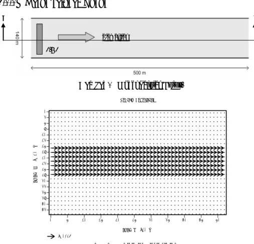
Gambar 1 Model Saluran Lurus.

0 5 10 15 20 25 30 35 40 45 50 0 3 5 8 10 13 15 18 20 23 25 28 30 33 35 38 40 43 ARAH X (x10 m) A RA H Y (x 10 m) = 0.26 VEKTOR KECEPATAN

Gambar 2 Vektor Kecepatan.

Pada kasus saluran lurus ini terlihat pergerakan salinitas sesuai dengan arah kecepatan, dengan kecepatan yang sama. Tampak bahwa pergerakan salinitas dipengaruhi oleh konveksi dan difusi, yang ditandai dengan pergerakan puncak dan penyebaran (distribusi) disertai penurunan puncak, dimana pergerakan puncak memiliki kecepatan yang sama dengan kecepatan aliran.

DISTRIBUSI SALINITAS DI SALURAN LURUS

-0.2 -0.1 0 0.1 0.2 0.3 0.4 0.5 0.6 2 4 6 8 10 12 14 16 18 20 22 24 26 28 30 32 34 36 38 40 42 44 46 48 50 52 GRID S A LI N ITA S menit ke-6 menit ke-12 menit ke-18 menit ke-24 menit ke-30 menit ke-36 menit ke-42 menit ke-48 menit ke-54 menit ke-60

4.1.2

Kasus Ekspansi Satu Sisi

Gambar 4 Model saluran ekspansi tiba-tiba.

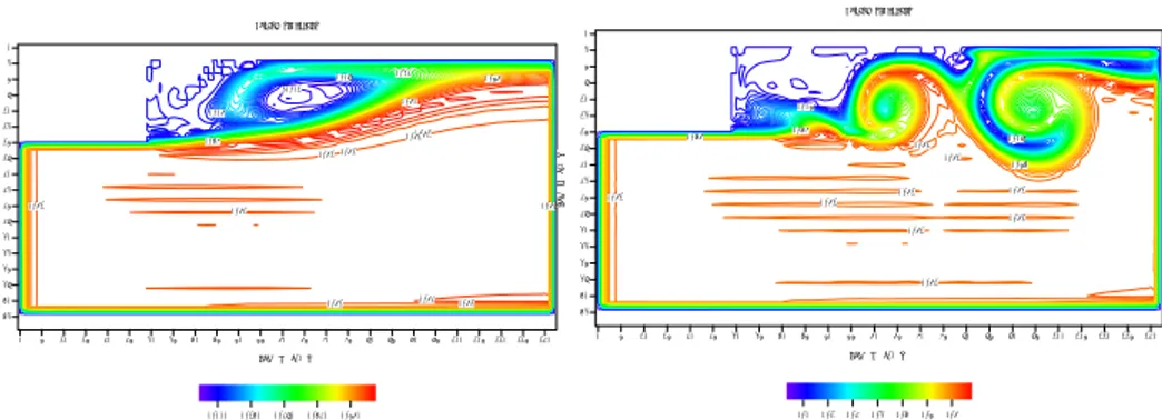
0 5 101520253035404550556065707580859095 100 105 110 115 120 0 3 5 8 10 13 15 18 20 23 25 28 30 33 35 38 40 43 ARAH X (x10 m) AR AH Y ( x 10 m) = 0.22 VEKTOR KECEPATAN 0 10 20 30 40 50 60 70 80 90 100 110 120 0 3 5 8 10 13 15 18 20 23 25 28 30 33 35 38 40 43 ARAH X (x 10 m) A RAH Y (x 10 m) = 0.24 VEKTOR KECEPATAN

Gambar 5 Vektor kecepatan pada jam ke-7 untuk kasus non turbulen (a) dan turbulen (b). 0.18 0.15 0.15 0.13 0.11 0.06 0.15 0.14 0.14 0.14 0.14 0.17 0.18 0.01 0.19 0.04 0.19 0.20 0.17 0.05 0 5 101520253035404550556065707580859095 100 105 110 115 120 0 3 5 8 10 13 15 18 20 23 25 28 30 33 35 38 40 43 Arah X (x10 m) A rah Y (x 10 m) MAGNITUDE KECEPATAN 0.01 0.08 0.08 0.00 0.04 0.06 0.10 0.10 0.03 0.00 _{0.15 0.24} 0.00 0.11 0.22 0.15 0.19 0.20 _0.20 0.19 _0.20 0.18 0.19 0.20 _0.18 0.20 0.20 0.15 0.20 0.20 0.19 0.180.18 0 6 12 18 25 31 37 43 49 55 61 67 74 80 86 92 98 104 110 116 123 0 3 5 8 10 13 15 18 20 23 25 28 30 33 35 38 40 43 ARAH X (x 10 m) AR AH Y (x1 0 m) MAGNITUDE KECEPATAN

Gambar 6 Kontur Kecepatan pada jam ke 7 untuk kasus non turbulen (a) dan turbulen (b).

0.61 0.08 0.32 0.56 0.60 -0.01 0.61 0.61 0.61 0.61 0.61 0.61 0.62 0.06 0.61 0.61 0.47 0.61 0.61 0 5 10 1520 25 30 35 40 4550 55 60 65 70 7580 85 90 95100105110115120 0 3 5 8 10 13 15 18 20 23 25 28 30 33 35 38 40 43 Arah X (x10 m) Arah Y ( x10 m) 0.000 0.140 0.280 0.420 0.560 Salinitas (ppt) KONTUR SALINITAS 0.05 0.47 0.46 0.08 0.61 0.61 0.54 0.61 0.61 0.61 0.61 0.61 0.61 0.61 0 5 10 15 20 25 30 35 40 45 50 55 60 65 70 75 80 85 90 95100105110115120 0 3 5 8 10 13 15 18 20 23 25 28 30 33 35 38 40 43 Arah X (x10 m) A ra h Y (x 10 m) 0.00.10.2 0.30.40.50.6 Salinitas (ppt)

Gambar 7 Kontur Salinitas pada jam ke -7 untuk kasus non turbulen (a) dan kasus turbulen (b).

Pada saluran ekspansi terlihat turbulensi terbentuk akibat ekspansi tiba-tiba pada dinding batas saluran. Pada model turbulen pola turbulensi menguat, terdapat peningkatan kecepatan, serta pembentukan pusaran-pusaran baru yang ukurannya lebih kecil terlihat lebih jelas dan stabil dibandingkan dengan hasil model non turbulen. Produksi turbulensi yang sangat tinggi (fenomena bursting)

terjadi secara repetitif dan berfluktuasi pada zona resirkulasi dengan frekuensi tertentu. Fenomena bursting ini ditandai dengan terbentuknya vorteks dan

terjadinya proses resirkulasi. Pusaran-pusaran yang besar terbentuk akibat kondisi batas (dalam hal ini dinding), sedangkan pusaran-pusaran yang kecil terbentuk oleh viscous force [14].

Pada aliran turbulen pemisahan struktur pola arus/kecepatan di tengah dan bagian sayap saluran terlihat sangat signifikan, begitu pula pusaran arus menjadi bentuk pola arus yang dominan di bagian sayap saluran. Pada aliran non turbulen pola pusaran arus di bagian sayap terlihat lebih lemah. Pola aliran sangat berpengaruh pada kecepatan penyebaran salinitas. Adanya turbulensi menyebabkan salinitas lebih cepat terdistribusi ke seluruh bagian saluran, jika dibandingkan dengan penyebaran salinitas pada aliran non turbulen. Hal ini disebabkan sifat difusif aliran turbulen yang mempercepat proses pencampuran

(mixing) berbagai kuantitas, termasuk massa (konsentrasi).

5

Kesimpulan

Pada kasus ekspansi tiba-tiba, model turbulen Kappa-Epsilon mampu memberikan pola arus yang lebih baik dibandingkan model non turbulen. Hal ini terlihat dengan munculnya fenomena bursting dan resirkulasi yang tidak

dapat dihasilkan oleh model non turbulen. Selain itu, model turbulen κ-ε telah dapat memberikan gambaran pola aliran yang lebih stabil pada aliran turbulen.

Selain itu model turbulen κ-ε juga memberikan pola penyebaran salinitas (konvektif dan difusif) yang lebih baik dan akurat dibandingkan model non turbulen.

Acknowledgement

Penelitian ini dilakukan dengan biaya DIKTI melalui program hibah Bersaing XII dan Hibah Pasca Sarjana P2M DIKTI 2007.

Daftar Pustaka

[1] Adam, E. W., J.P. Johnston and J.K. Eaton, Experiments on the structure

of Turbulent Reattaching Flow, ReportbMD-43, Thermosciences

division-Dept of Mech Eng.-Stanford Univ., California, 1984.

[2] M. Syahril B. K. And Claud Rey, Visualization of Backward Facing Step

Flows, Proc. of Euromech 276, Dynamics of The Urban Atmosphere,

Nantes, Perancis, 1992.

[3] Bradshaw, P. and F.Y. Wong, The Reattachment and Ralaxation of

Turbulent Shear Layer, JFM, 52, pp113-135, 1972.

[4] Chandrasuda C. and Bradshaw, Turbulent Structure of Reattaching

Mixing Layer, JFM, 110, pp171-194, 1981.

[5] Hunt, J.C.R., Coherent Structures-Comments on Mechanism, Seminar

Proceeding of Von Karman Institute for Fluid Dynamics, Lecture Series 1989-03, 1989.

[6] Hussain, A.K.M.F and W.C. Reynolds, The Mechanism of Organized

Wave in Turbulent Shear Flow, JFM, 41, part2, 241-258, 1973.

[7] M. Syahril B.K, R.A. Rahayu, H. Kardana and M. Cahyono, Numerical Simulation of Two Dimensional Turbulent Flow in Division Box of an

Irrigation Channel Based on

κ

−

ε

Model, Proceeding of International

conference on Fluid and Thermal Energy Conversion, Jakarta, December 10th_-14th_{, 2006.}

[8] M. Syahril B.K, R.A. Rahayu, H. Kardana and M. Cahyono,

Development Of Turbulent

κ

−

ε

Model for Assesing Water Quality

Distribution in Reservoir, Research Report, Asahi ResearchGrant, 2006.

[9] M. Syahril B. K., M Cahyono & Eka O. N., Development Study of Turbulent K-E Model for Recirculation flow I: Two Dimension Flow in

Reservoir, Proceeding ITB, 2004.

[10] M. Syahril B. K., M. Cahyono, Hasan B & Noorsalam, Optimalization on

Water Distibution for Fishery Ponds in Indramayu, research report, Dinas

Perikanan TK II Indramayu-LP ITB, 1999.

[11] Launder, B.E., and Spalding, D. B., Lectures in Mathematical Models and Turbulence, Academic Press Inc, New York, 1972.

[12] Chapman, R.S, and Kuo, C.Y., Application of the two equation κ-ε

Turbulence Model to a Two Dimentional, Steady, Free Surface Flow Problem with Separation, International Journal for Numerical Methods in Fluids, Vol.5, 257-268, 1985.

[13] Rastogi, A.K., and Rodi, W., Prediction of Heat and Mass Transfer in Open Channels, J. Hydraulics Div., ASCE, 104 (HY3), 397-420, 1978. [14] Rastogi, A.K., Private communication with W. Rodi (1980). Turbulence

Models and Their Application in Hydraulics: a State of The art review, Presented by IAHR-Section on Fundamentals of Divison II: Experimental and Mathematical Fluid Dynamics, Delft, Netherland, P.50, 1978.

[15] Abbott, M.B., Basco, D.R., Computational Fluid Dynamics an

Introduction for Engineers, Longman Scientific & Technical, England,

1989.

[16] Anderson JR, J.D., Computational Fluid Dynamics, McGraw-Hill

International Editions, New York, 1995.

[17] Blackwelder, R.F. and Haritonidis, Scaling of Bursting Frequency in

Turbulent boundary Layer, JFM, 132, 87-103, 1983

[18] B. Mohammadi & O. Pironneau, Analysis of The K-Epsilon Turbulencve

Model, John Wiley & Sons, 1994.

[19] Chapra, Steven C., Surface Water Quality Modelling, The McGraw-Hill

Companies Inc., Si

[20] Driver, D.M and H. Lee Seegmiller, Features of Reattacing Turbulent

Shear Layer in Divergent Channel, AIAA Journal, 23(21), 1985.

[21] Falconer, R.A., Guiyi, Li, Modelling Tidal Flows in an Island’s Wake

Using a Two Equation Turbulence Model, Journal of Fluid Mechanics,

1992, 43-53.

[22] Fletcher, C.A.J., Computational Techniques for Fluid Dynamics Volume

I-II, Second Edition, Springer-Verlag, London, 1990. [23] Hirt, C.W., Turbulence Modelling, Flow Science, Inc.

[24] Hoffman, J.D., Numerical Methods for Engineers and Scientists,

McGraw-Hill, Singapore, 1993.

[25] Hussain, A.K.M.F and A.R. Clark, On the Coherent Structure of the

Axisymmetric Mixing Layer: a Flow Visualization Study, JFM, 104,

263-294, 1981.

[26] Kim, J.J, On the Structure of Wall Bounded Turbulent Flows, Physic of

Fluids, 26(8), 2088-2092, 1983.

[27] Launder, B.E., and Spalding, D. B., Thenumerical Computation of

Turbulent Flows, Computer Method in applied Mechanics and engineering, 3, 269-289, 1974.

[28] M. Syahril Badri K., M Martono, Hang Tuah & S Legowo, Experimental Study on Spectral Behaviour on Backward Facing Step Flows: Rough

Wall Boundary Layer Cases, The Sixth Asian Congress of Fluid

Mechanics,Singapore, pp. 1376-1379, 1995.

[29] M. Syahril B. K. And Hang Tuah, Backward Facing Step Flow: The

Effect of Initial Condition on The reattachment of Turbulent Shear

Layer, Proc. of 1st International Symposium on Fluid Dynamic & Energy,

Bali Indonesia, 1994.

[30] Ni, H.Q., Shen, Y.M., Zhou, L.X., Duan, J.H., Numerical Simulatoin of

Multiple Circulating Flows Using A Depth-Averaged κ-ε Turbulence

Model For The Entire Field, The Sixth Asian Congress of Fluid

Mechanics,Singapore, pp. 801-803, 1995.

[31] Press, W.H., Flannery, B.P., Teukolsky, S.A., Vetterling, W.T.,

Numerical Recipes The Art of Scientific Computing, Cambridge

University Press, New York, 1986.

[32] Rijn, Leo C. van, Principles of Fluid Flow and Surface Waves in River,

Estuaries, Seas, and Oceans, Aqua Publications, The Netherlands, 1990. [33] Strickland, J.H and Simpson, R.L, Bursting Frequencies Obtained From

Wall Shear Stress Fluctuations in a Turbulent Boundary Layer, Physics

Fluids, 18(2), pp 306-308.

[34] Westphal, R.V, J.P. Johnston and J.K. Eaton, Experimental Study of Flow

Reattachment in a Single Sided Sudden Expansion, NASA Contractor

Report 3765, 1984.

[35] Wilcox, C. David, Turbulence Modeling For CFD, DCW Industries, Inc,

California, 1994.

[36] Younus, Muhammad, Computation of Free-Surface Flow By Using

Depth-Averaged κ-ε Turbulence Model, Disertasi, Department of Civil