An alternative derivation of the shallow water equations.

(1)

VoI. 03

No.

01

Januari

ztll

ISSN:2087-5126

#-::tc

Published

by

(2)

Bulletin

of

Mathernatics

(Inrlonesian Matheruatical Sociertl' Acelr - North Sr:.rnatera)

c/o Departrnent

of

N{atheruatics.

L}nivcrsitl' of

Surnatera

Utara

.]alan

Bioteknologi

1. Karnpus USLI. l,Iedan 20155. Indonesia E-mail:bulletirrrlallrrllaticsl0raloo.corrr Websitc: hl.1p:/7'irrlonrs-rri.lstrrnxt.org & hitp:/ll;rrl)-rrrLh.org

Editor-in-Chief:

Hernrarr l.{awengkang, Deytt. of

kfatlt.,

{lni,rersi,ty

af

Srtlnlrte:a t}taxt,, Mtilsn,,

In-donesia

&{anagir:g

Editor:

Hizir Sofyan, Dr:pt. of klatl't.. LTnsyiah Llniuersity, Banda A*:./t,, In,danesitr'

Associatc Editors:

Algebra and

Geornetry:

Iraw.*y.

Ilept.

of Math,., Institr-tt Teknal,ogi Btt'ndung, Bon,dun,g. fndonesin

Pangeran Sialipar. Dept. a{ }lIath., lJni'aersitg o{ Su,m.a,tera Uto,r'*,, l{ed,an, IrLd,r:ne'

sia,

Analysis:

Oki ldeswan, Dept,. r;l Mc,th,., Insti,tut "kknalag'i l3o'nd,urr4;. /3*'ndu*9, !'ntk:nesia L{aslina Dalus, Sch,osl oJ'},t*,th. Scir:nr;.es. tln'rL;ers'}ii Kr:ba'n,gs*o,n, rt.lala;qs|a" Bu,rt,gi,.

.l;1nItt) ,\tatuas 10.

Applied Mathematics:

Tarmizi Usman, Dept. of Math,., Unsyiatt {.initersity, Bd'ntla Ar:t*,, In,rl,onesirt Inrrar, Dept. of bIath., fr.iax, {Jnn:trsity, Pekrtn,baru, Indr;rtesia

Discrete Mathematics

&

Combinatorics:

Surahmat, De.pt. of

Math.

liducation,, {slr,m,ic {,:ni'r;rt'sity of Ma,lung, *{olanq.

Irt-rlonesia

Saib Suwilo. Deyt. af trIath., Liniuers'ity af Surna,tera {ltara" Merlon.. I'ntlonesio,

Statistics &

Probability

Theory:

I liyouran Buriianlara. Dr:2tt. o.f Stat., InstittLt Tekuologi Se'pululr, Naperrrbcr, S'urtba'yo,.

f....t....,... 1utl,t/ur,)(tl

(3)

Bulleti,n

of

Mathemat'ics

ume

anuary

Kolmogorov

Complexity:

Clustering Objects and

Similarity

Mahyuddin

K. M.

Nasution

1

htzzy

Neighborhood

of

Cluster

Centers

of Electric

Current

at Flat

EEG

During Epileptic

Seizures

Muhammad

Abdy

and

Tahir

Ahmad

LT

Membanding

Metode

Multiplicative

Scatter Correction

(MSC)

dan Standard

Normal

Variate (SNV)

Pada

Model

Kalibrasi

Peubah Ganda

Arnita

dan

Sutarman

25

2-Eksponen

Digraph Dwiwarna

Asimetrik

Dengan

Dua

Cycle yang Bersinggungan

problem

Mardiningsih,

Saib Suwilo dan

Indra

Syahputra

39

Analisis

Ketegaran Regresi

Robust

Terhadap

Letak

Pencilanl Studi

Perbandingan

Netti

Herawati,

Khoirin

Nisa dan

Eri Setiawan

49

A

Unified

Presentation

of

Some

Classes

p-Valent

Functions

with

Fixed

Second

Negative Coefficients

Saibah

Siregar

61

Peringkat

Efisiensi Decision

Making

Unit

(DMU)

dengan

Stochastic

Data

Envelopment

Analysis (SDEA)

Syahril

Efendi

69

An

Alternative

Derivation of The

Shallow

Water

Equations

Sudi

Mungkasi

79

Model

Pemrograman Stokastik dengan Scenario Generation

(4)

Bulletin of Mathematics

Vol. 03, No. 01 (2011), pp. 79–85.

AN ALTERNATIVE DERIVATION OF THE

SHALLOW WATER EQUATIONS

Sudi Mungkasi

Abstract. _{The one dimensional shallow water equations consist of the equation}

of mass conservation and that of momentum conservation. In this paper, those equations are derived. We utilize a constant approximation of integration in the derivation. We call our derivation an alternative derivation since it is different from the classical derivation. The classical derivation of the shallow water equations involves a velocity-potential function, while our derivation does not.

1. INTRODUCTION

The shallow water equations, or SWE for short, model shallow water flows as the name suggest. These equations are according to the transport of mass and momentum, and based on conservation laws. These equations form a nonlinear hyperbolic system, and often admit discontinuous solution even when the initial condition is smooth. They have been widely used for many applications, for example: dam-breaks, tsunamis, river flows, and flood inundation. The SWE also known as the Saint-Venant system, for the one dimensional case, can be written as two simultaneous equations

ht+ (hu)x = 0, (1)

Received 21-01-2011, Accepted 31-01-2011.

2010 Mathematics Subject Classification: 76B07, 76B15.

Key words and Phrases: shallow water equations, conservation of mass, conservation of momen-tum.

(5)

[image:5.595.172.423.126.263.2]

Sudi Mungkasi – An alternative derivation of the shallow water equations 80

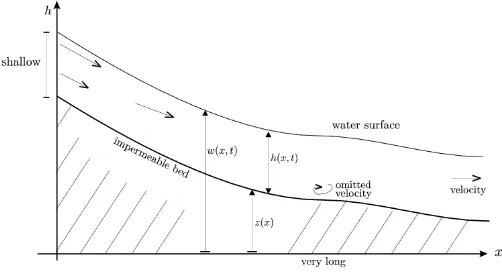
Figure 1: Shallow water flow in one-dimension

(hu)t+ (hu2+

1 2gh

2₎

x =−ghzx. (2)

Here, we have that: xrepresents the distance variable along the water flow,t

represents the time variable,z(x) is the fixed water bed,h(x, t) is the height of the water at pointxand at timet, andu(x, t) denotes the velocity of the water flow at point x and at time t. In addition, g is a constant denoting the acceleration due to the gravity. The shallow water flow is illustrated in Figure 1, where the water stagew is defined by w(x, t) =z(x) +h(x, t) .

In this paper, we present an alternative derivation of the one dimen-sional SWE (1), (2) using a constant approximation of integration. We call our derivation as ”an alternative derivation”, because our derivation is dif-ferent from the classical derivation, which usually uses a velocity-potential function (see Stoker [3] for the classical derivation). Note that LeVeque [2] has derived some conservation laws, but also in a different way. We start from an arbitrary control volume, then derive the shallow water equations based on the considered control volume. Since the control volume is arbi-trary, the shallow water equations hold for an arbitrary domain.

This paper is organized as follows. Section 2 recalls a constant ap-proximation for integral form, and also presents the derivation of the SWE consisting of equation (1) of mass conservation and equation (2) of momen-tum conservation. We provide some concluding remarks in Section 3.

2. DERIVATION OF THE SWE

(6)

[image:6.595.200.395.125.202.2]

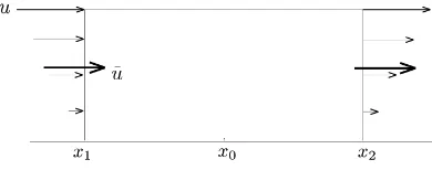
Figure 2: The inflow and outflow of the control volume

form. The properties of the approximations are given in the following the-orem, where the proof has been provided by Laney [1, pp.176–177].

Theorem 2.1 _{Suppose that we are given an arbitrary interval} _[_x₁_{, x}₂_]_{. Let}

∆x = x2 −x1. If x0 ∈ [x1, x2] but x0 is not the centroid of the interval,

then _Z

x₂ x1

f(x) dx=f(x0)∆x+O(∆x2). (3)

If x0 is the centroid of the interval[x1, x2], then

Z x₂ x₁

f(x) dx=f(x₀)∆x+O(∆x3). (4)

2.1. Conservation of mass

Conservation of mass means that the mass is neither created nor de-stroyed. Several assumptions, involved in the derivation of the equation of mass conservation, follows. First, the water flow is assumed to be laminar that is the turbulent velocity is neglected. Second, the water is incompress-ible so that the density,ρ, of the water at each point is constant. In addition, because the conservation of mass is applied and it is assumed that the water bed is impermeable, the mass in any control volume can change only due to the flow acrossing the end points of the control volume.

The total mass m of water in an arbitrary control volume [x1, x2] is given by

m=

Z x₂ x1

ρh(x, t) dx (5)

(7)

The rate of flow of water past any point (x, t) over the depth is called themass flux which is given by

mass flux =ρh(x, t)u(x, t). (6)

Using (6), we obtain that the rate of change of the total mass is

d dt

Z x₂ x1

ρh(x, t) dx=ρh(x₁, t)u(x₁, t)−ρh(x₂, t)u(x₂, t). (7)

For smooth solutions, (7) is equivalent to

Z x2

x₁

h(x, t+ ∆t)dx =

Z x2

x₁

h(x, t)dx+

Z t+∆t

t

h(x1, s)u(x1, s)ds

− Z t+∆t

t

h(x2, s)u(x2, s)ds . (8)

Equation (8) means that the mass at time step t+ ∆t is equal to the mass at timetadded by the total amount of mass moving into the control volume during ∆t-period, as illustrated in Figure 2.

Let ∆x and ∆t be small quantities. Using a constant approximation (4) of integration, we can rewrite equation (8) as

h(x, t+ ∆t)∆x = h(x, t)∆x+h(x−∆x

2 , t)u(x− ∆x

2 , t)∆t

−h(x+ ∆x

2 , t)u(x+ ∆x

2 , t)∆t

+O(∆t3) +O(∆x3) (9)

which can be rewritten as

h(x, t+ ∆t)−h(x, t) ∆t =−

(hu)|₍_x₊∆x

2 ,t)−(hu)|(x−∆

x

2 ,t)

∆x , (10)

in whichO(∆t3) andO(∆x3) terms are neglected. As ∆xand ∆tapproach zero, equation (10) becomes

ht+ (uh)x= 0 (11)

Equation (11) is then called the equation of mass conservation.

(8)

[image:8.595.172.423.127.290.2]

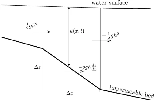
Figure 3: Pressure in a slope area

In this subsection, the conservation of momentum equation using Newton’s second law of motion is presented. The law can be mathematically written as

F = dp

dt , (12)

where the inertial forceF is defined as the rate of change of the momentum

p with respect to timet.

The total momentum of water movement in any control volume from

x1 tox2 at timet is

p(t) =

Z x₂ x₁

ρh(x, t)u(x, t) dx . (13)

The forces at points x1 and x2 over the depth at time tare

F1(t) = 1 2ρgh

2₍_x

1, t) (14)

and

F₂(t) =−1

2ρgh 2₍_x

2, t) (15)

respectively, where g > 0 is constant denoting the acceleration due to the gravity as we have stated in the introduction section. Furthermore, the force over ∆z as shown in Figure 3 is

(9)

or can be written as

∆F3 =−ρgh(x, t) ∆z

∆x∆x (17)

and therefore the force over the bottom of the control volume is

F3 =

Z x2

x₁

−ρgh(x, t)zxdx (18)

Hence, the total force over the control volume denoted by F is the sum of

F1,F2, and F3, that is,

F = 1 2ρgh

2₍_x 1, t)−

1 2ρgh

2₍_x 2, t)−

Z x₂ x₁

ρgh(x, t)dz

dxdx . (19)

Using Leibniz’s rule for differentiation under the integral sign, we ob-tain that the first derivative of p with respect totis

dp dt =

d dt

Z x₂ x₁

ρh(x, t)u(x, t)dx

=

Z x₂ x₁

∂

∂tρh(x, t)u(x, t) dx

+ρh(x2, t)u2(x2, t)−ρh(x1, t)u2(x1, t). (20)

According to Newton’s second law (12) of motion, we have that the result in equation (20) is equal to that in equation (19). Hence, for ∆t-period it follows that

Z t+∆t

t

Z x2

x₁

(ρhu)tdx dt+

Z t+∆t

t

ρh(x2, t)u2(x2, t) dt

− Z t+∆t

t

ρh(x1, t)u2(x1, t)dt=

Z t+∆t

t

1 2ρgh

2₍_x 1, t) dt

− Z t+∆t

t

1 2ρgh

2₍_x

2, t) dt−

Z t+∆t

t

Z x₂ x1

ρgh(x, t)zx dx dt (21)

Using a constant approximation (4) of integration, we can rewrite equa-tion (21) as

(hu)t+ (hu2+

1 2gh

2₎

x =−ghzx, (22)

in which O(∆t3) and O(∆x3) terms are neglected. This last equation is called the equation of momentum conservation.

(10)

We have derived the one dimensional shallow water equations, which con-sist of the equation of mass conservation and the equation of momentum conservation, using a constant approximation of integration. Our presenta-tion suggests that higher dimensional shallow water equapresenta-tions can also be alternatively derived using a similar technique.

ACKNOWLEDGEMENT

The author thanks Associate Professor Stephen Roberts at The Australian National University (ANU) for his advice. This work was done when the author was undertaking a masters program at the ANU.

References

[1] C. B. Laney. 1998.Computational Gasdynamics, Cambridge University Press, Cambridge.

[2] R. J. LeVeque. 2002. Finite-Volume Methods for Hyperbolic Problems, Cambridge University Press, Cambridge.

[3] J. J. Stoker. 1957. Water Waves: The Mathematical Theory with Ap-plication, Interscience Publishers, New York.

Sudi Mungkasi_{: Department of Mathematics, Mathematical Sciences Institute,}

The Australian National University, Canberra, Australia; Department of Mathe-matics, Faculty of Science and Technology, Sanata Dharma University, Yogyakarta, Indonesia.