THE INFLUENCE OF FINANCIAL RATIO ON PROFIT GROWTH IN MANUFACTURING COMPANIES LISTED ON IDX FOR PERIOD 2008 TO 2012
THESIS
Submitted as Partial Fulfillment of Requirement for the Undergraduate Degree in Accounting Department Faculty of Economics
By:
POPY ANA PUTRI
0910534036
INTERNATIONAL ACCOUNTING DEPARTMENT
FACULTY OF ECONOMICS
ANDALAS UNIVERSITY
ACCOUNTING DEPARTMENT
FACULTY OF ECONOMICS
ANDALAS UNIVERSITY
THESIS APPROVAL LETTER
Herewith, Head of Accounting Department, Head of Accounting International Program and Thesis Advisor, stated that :
Name : POPY ANA PUTRI
Student’s ID Number : 0910534036 Field of Study : Accounting
Degree : Bachelor Degree of Economics (S1)
Thesis Title : The Infuence of Financial Ratio on The Profit Growth in Manufacturing Companies Listed on IDX for Period 2008-2012
Has already passed the thesis seminar on Friday November 29th, 2013 based on procedures and regulations prevailed in the Faculty of Economics, Andalas University.
Padang, January16 2014 Thesis Advisor
Drs.Riwayadi, MBA, Ak, CRSR
NIP.196412281992071001
Approved by :
Head of Accounting Department Head of AccountingInternational Program
Dr. Efa Yonnedi SE, MPPM,Ak Rayna Kartika, SE, M.Com, Ak
No.Alumni Universitas Popy Ana Putri No.Alumni Fakultas
BIODATA
a). Tempat/Tgl Lahir : Bukittinggi/13 Agustus 1991 b). Nama Orang Tua : Musdawarman/Yuniarti c). Fakultas : Ekonomi d). Jurusan : Akuntansi e). No.BP : 0910534036 f). Tgl Lulus : 7 Januari 2014 g). Predikat Lulus : Sangat Memuaskan h). IPK : 3,27 i). Lama Studi : 4 tahun 5 bulan j). Alamat Orang Tua : Bukittinggi
The Infuence of Financial Ratio on The Profit Growth in Manufacturing Companies Listed on IDX for Period 2008-2012
Thesis By : Popy Ana Putri
Thesis Advisor : Drs.Riwayadi, MBA, Ak, CRSR
ABSTRACT
This research examines the effects of Working Capital to Total Asset (WCTA), Current Liabilities To Inventory (CLI), Operating Income to Total Assets (OITL), Total Asset Turnover (TAT), Net Profit Margin (NPM) dan GrossProfit Margin(GPM) to profit growth of manufacture company.
The sampling technique used in this research is purposive sampling, with some criteria, those are: (1) the manufacture company listed in IDX in research period and still operating consistenly in the research period; (2) issuing of financial statement as the research period; (3) the manufactur company having the positive profit. The result of this research shows that the data has fulfill the classical asumption, such as: no multicolinearity, no autocorrelation, no heteroscedasticity and distributed normally. From the hyphothesis testing, found that partially Gross Profit Margin (GPM) variable, has a positive and significant influence on profit growth of manufacture company, while Working Capital to Total Asset(WCTA), Current Liabilities To Inventory(CLI), Operating Income to Total Assets (OITL), TotalAsset Turnover (TAT), and Net Profit Margin (NPM) don’t have influence on profit growth of manufacture company. From the research also known that those six variable (WCTA, CLI, OITL, TAT, NPM, and GPM) simultaneously have an influence on profit growth of manufacture company. All of independent variables in this study are only accounted for 6,7% that affect on dependent variable and the remaining 93,3% is influenced by other factors that are not included in the regression model as shown in the adjusted R2 value.
Keywords: Working Capital to Total Asset (WCTA), Current Liabilities ToInventory (CLI), Operating Income to Total Assets (OITL), Total Asset Turnover(TAT), Net Profit Margin (NPM), Gross Profit Margin(GPM) and profit growth.
Skripsi telah dipertahankan di depan sidang penguji dan dinyatakan lulus pada tanggal 29 November 2013, dengan penguji :
Ketua Jurusan Akuntansi: Dr. Efa Yonnedi SE, MPPM,Ak
ACKNOWLEDGMENTS
Alhamdulillahirabbilalamin. First of all I would like to express my deepest gratitude to Allah SWT, for the bless and guidance, therefore I could accomplish my thesis as partial fulfillment of the requirement for the undergraduate Degree in Accounting Department, Faculty of Economics Andalas University, Padang. And of course to my prophet Muhammad SAW.
Later, the gratitude is also dedicated for people who give support, advice, and help to compile the thesis who I can not mention one by one. Hence, I would like to express me deepest thanks to :
1. My beloved family Mom and Dad, my brother and my sister. There is no word that can express my greatfulness to my family, thank you so much for everything, a grace that is not measurable if someday be able to give happiness to my beloved family. Amin..
2. Efa Yonnedi, SE, MPPM, Ak, Phd as the Head of Accounting Department and also Firdaus, SE, Msi, Ak as the Secretary of Accounting Department, for every help during my college life.
3. My best gratitude to Drs.Riwayadi, MBA, Ak, CRSR as my thesis advisor. Thank you so much for your helpful, advice, guidence, time and also the lesson.
5. All the lectures of Economics Faculty especially Accounting and International Accounting Class, I am really proud of being a part of this class.
6. Staff of Accounting bureaucracy, Da Ari and Ni Eva, you make everything easy to student and also me.
7. To my beloved girls Sari, Visri, Indah and my roomate Fizy who already gave me such many unforgettable experiences, life lessons..so many happiness and sadness we spent together. Hopefullythe success will be with us and this friendship will never end. Hugs and kisses..:) :*
8. To all my friend in International Accounting Class 09 for all the support and pray for me. I do hope all the best for all of you guys.
9. Special gratitude to my soul mate Baim. you have colored my life and fill my days with happiness..thank you for everything baim..your support, understanding and love..hope we can make our dreams come true. Amin..^_^
Padang, January16 2014
CONTENTS
CONTENTS... i
TABLES ……….... v
FIGURES ………. vi
CHAPTER I: INTRODUCTION 1.1 Background... ... 1
1.2 Formulation of The Problem... 5
1.3 Purpose and Usability ... 6
1.3.1 Research Objectives... 6
1.3.2 The Usefulness of The Research... 7
1.4 Writing Systematic………... 7
CHAPTER II: LITERATURE REVIEW, THEORETICAL FRAMEWORK AND HYPOTHESIS 2.1 Literature review ... 9
2.1.1 Financial Statement Analysis... 9
2.1.2 Financial Ratio Analysis ... 11
2.1.3 Profit Growth ... 17
2.2 Previous Research ... 18
2.3 Theoretical Framework ……… 25
2.4.1 Relationship Working Capital to Total Assets on Profit Growth 26
2.4.2 Relationship Current Liability to Inventory on Profit Growth... 27
2.4.3 Relationship Operating Income to Total Liabilities on Profit Growth……….... ... 27
2.4.4 Relationship a Total Assets Turnover on Profit Growth... 28
2.4.5 Relationship Net Profit Margin on Profit Growth ... 28
2.4.6 Relationship Gross Profit Margin on Profit Growth... 29
CHAPTER III: RESEARCH METHODOLOGY 3.1 Type of Research ... 30
3.2 Research Variables and Operational Definition of Variables...…….... 30
3.2.1 Research Variables ... 30
3.2.2 Operational Definition of Variables ... 31
3.2.2.1 Dependent Variable ... 31
3.2.2.2 Independent Variable ... 31
3.3 Population and Sample ... 35
3.3.1 Population ... 35
3.3.2 Samples ... 35
3.4 Data ... 36
3.4.2 Methods of Collecting Data ... 36
3.5 Classic Assumption Test ... 36
3.5.1 Normality Test ... 36
3.5.2 Multicollinearity Test... 38
3.5.3 Autocorrelation Test ………... 39
3.5.4 Heterocedasticity Test ………. 40
3.6 Analysis Techniques ... 40
3.7 Hypothesis Testing ... 41
3.7.1 Coefficient Determination (R2) ... 41
3.7.2 F Test ... 42
3.7.3 t Test ... 43
CHAPTER IV: RESULTS AND DISCUSSION 4.1 General Overview and Descriptive Data of Research Object……… 45
4.1.1 Research Object Overview ... 45
4.1.2 Descriptive Data ……….…………... 46
4.2 Classic Assumption Test ……….…….….... 48
4.2.1 Normality Test ………. ... 48
4.2.2 Multicollinearity Test ………... 52
4.2.3 Autocorrelation Test ………..….. 53
4.3 Multiple Regression Analysis Result ………..….. 55
4.3.1 Coefficient of Determination (R2) ……….… . 56
4.3.2 F Test ……….... ... 56
4.3.3 t Test ………... 57
4.4 Hypothesis Testing ………... 58
4.4.1 Testing Hypothesis 1……….... 58
4.4.2 Testing Hypothesis 2 ………... 59
4.4.3 Testing Hypothesis 3 ………... 59
4.4.4 Testing Hypothesis 4 ………... 60
4.4.5 Testing Hypothesis 5 ………... 61
4.4.6 Testing Hypothesis 6 ………... 62
4.5 Discussion ………... ... 61
CHAPTER V: CONCLUSIONS 5.1 Conclusion ……… 65
5.2 Implication………... 66
5.3 Limitation ……… 66
5.4 Suggestion ……….. 67
REFERENCES……….. 68
TABLES
Table 2.1 Summary of Previous Research ……….. 22
Table 3.1 Operational Definition ……….…... 34
Table 3.2 Autocorrelation ………... 39
Table 4.1 Selection Sample ………... 45
Table 4.2 Descriptive Statistics ………..…... 47
Table 4.3 Normality Test Result Beginning Data ………. 49
Table 4.4 Normality Test Result Ending Data……….. 50
Table 4.5 Multicollinearity Test Result………... 52
Table 4.6 Autocorrelation ………... 53
Table 4.7 Autocorrelation Test Result ……….. 54
Table 4.8 R2Value ………..…... 56
Table 4.9 F test Result ………..….... 57
FIGURES
Figure 2.1 Theoretical Framework ………... 26
Figure 4.1 Graph Plot ……….………….……... 51
Figure 4.2 Histogram Plot ……….... 51
CHAPTER I
INTRODUCTION
1.1 Background
The success of an enterprise is measured based on its performance. The company's performance can be assessed through financial statements presented on a regular basis every period (Juliana and Sulardi, 2003). Brigham and Enhardt (2003) stated that the accounting information on the activities of the company's operations and financial position of the company can be obtained from the financial reports. Accounting information in financial statements is very important for the business person such as investors in decision-making. Investors will invest in companies that can provide a high return.
earnings. This is according to research by Machfoedz (1994) and Ediningsih (2004) show that significant negative effect CLI to predict a profit growth in coming years. This means that the company cannot make its debt to gain profit. However, research Takarini and Ekawati (2003) showed that the CLI does not influence significantly to predict profit growth one year ahead.
OITL is the ratio between operating profit before interest and taxes (i.e. the result of the reduction in net sales minus the cost of goods sold and operating expenses) to total debt (Riyanto, 1995). The larger the OITL, pointed out that the revenue generated from sales activities than the total debt, meaning that the companies is able to pay their debt. Thus the continuity of the company's operations will not be disrupted, so that earned income be increased and profits obtained huge. Mahfoedz (1994) and Ediningsih (2004) in his research showed that significant positive effect OITL predicts profit growth for one year to the next. While research and Takarini Ekawati (2003) and Suwarno (2004) indicates that no effect significant OITL predicts profit growth for one year to the next.
The research by Ou (1990) and Asyik and Sulistyo (2000) show that the positive effect of TAT significant profit growth. While the study conducted by Suwarno (2004), Takarini and Ekawati (2003), Juliana and Sulardi (2003) and Meythi (2005) indicates that TAT does not influence significantly to earnings growth. Asyik and Soelistyo (2000) in his research showed that the ratio of profitability that influence significantly to profit growth is the Net Profit Margin (NPM) and the Gross Profit Margin (GPM). NPM is a comparison between the net profit after taxes (i.e. profit before income tax is reduced by income tax) of net sales. This ratio measures the company's ability to generate revenue to achieved net sales company (Riyanto, 1995). The higher the NPM shows that increasing net profit achieved the company against net sales. Increasing NPM will improve the attraction of investors to invest its capital, so that the company's earnings will increase. Mahfoedz (1994), Asyik and Soelistyo (2000), and also Suwarno (2004) in his research suggests that the positive influence of NPM significant profit growth one year ahead. However, research results from Usman (2003), Meythi (2005), Takarini and Ekawati (2003) and Juliana and Sulardi (2003) showed that the NPM has no effect against the significant profit growth one year ahead.
showed that the GPM has no effect against the significant profit growth one year ahead. Based on empirical evidence that links between financial ratios (WCTA, CLI, OITL, TAT, NPM and GPM) against earnings growth (growth of Earning After Tax) still shows different results, then this study examines how the influence of the ratio of these financial-ratio of profit growth especially in the manufacturing sector in Indonesia Stock Exchange (IDX) of the period 2008 to 2012.
Selection of manufacturing companies in IDX because the manufacturing industry is the most industry many listed in IDX. Until now, the economy of Indonesia has not fully recovered from the economic crisis that faced Indonesia at the domestic level since mid-1997 and even in 2008 has the global economic crisis which impacted to the economy of Indonesia, therefore it is expected in 2008 to 2012 can improve economic conditions and profit growth will increase.
1.2 Formulation of the problem
This research was conducted to examine the influence of the WCTA, CLI, OITL, TAT, NPM and GPM of profit growth in the future in manufacturing companies registered in IDX period 2008 to 2012, so that the research question can be derived as follows:
1. How does the WCTA influence the profit growth at the company's manufacturing in the future?
3. How does the OITL influence the profit growth at the company's manufacturing in the future?
4. How does the TAT influence the profit growth at the company's manufacturing in the future?
5. How does the NPM influence the profit growth at the company's manufacturing in the future?
6. How does the GPM influence the profit growth at the company's manufacturing in the future?
1.3 Purpose and Usability
1.3.1. Research Objectives
The purpose of doing this research is:
1. Analyze the effect on profit growth against the WCTA manufacturing company.
2. Analyze the influence of the CLI to profit growth at the company's manufacturing.
3. Analyze the effect on profit growth against OITL manufacturing company.
4. Analyze the effect of TAT to profit growth at the company's manufacturing.
5. Analyze the influence of NPM to profit growth at the company's manufacturing.
1.3.2. The Usefulness of The Research
This research is expected to be beneficial to: 1. For Issuers
The results of this research are expected to be used as one of the basic considerations in decision-making in the areas of finance, especially in order to maximize the profit of the company having regard to the factors examined in this study.
2. For investors
The results of this research are expected to be used as a consideration in the decision making investments in manufacturing companies in Indonesia stock exchange (IDX).
1.4 Writing Systematic
The writing systematic of this study is divided into five chapters and each chapter divided into some subchapter. The first chapter are describes about the research backgrounds, problem definitions, research objectives, research benefits, and writing systematic.
The second chapter is literature review, theoretical framework and hypothesis that discuss about the theoretical analysis of this study that gathered from some sources, such as books, journals, internet, and previous research and discuss about hypothesis development.
definition and measurement, types of data, data collection method, data analysis method, classical basic assumption and hypothesis testing which used to analyze the data and any information needed.
Chapter fourth describes the result of research based on the data and information gathered related with problems definitions.
CHAPTER II
LITERATURE REVIEW
2.1 Literature Review.
2.1.1 Financial Statement Analysis
According to the Hanafi and Halim (2005), there are three forms of financial statements i.e. Statement of Financial Position, Income Statement, and Cash Flow statement.
(1) Statement of Financial Position
Statement of Financial Position, also known as the Balance Sheet, presents the financial position of an entity at a given date. The statement of financial position is a systematic report on assets, debt as well as the capital of a company on a particular date/time. The statement of financial position is made up of three main parts, namely assets, liabilities and capital. Assets consists of :
a) Current assets
b) Fixed assets
Fixed assets are intangible wealth the company money and could be disbursed in long-term (over one year). For example: bonds, land, buildings and machinery.
Liabilities is all the company's financial obligations to the other party that has not been fulfilled. Liabilities is a source of funds/capital companies that derived from the lender. Liabilities can be divided into two (Ang, 1997):
a) Current liabilities
Current liabilities are liabilities that maturities of less than one year. For example: short-term bank loans, notes payable and account payables (a liabilities arising from a purchase of goods in credit).
b) Non-current liabilities
Non-current liabilities is a liability maturities of more than one year. For example: bank loans, long term note payables, bonds liabilities and debts to shareholders.
Capital or equity is right or part owned by the owner of the company indicated in the capital post, surplus assets and retained earnings. Can also meant an excess value of assets owned by the company to the rest of what he owes (Munawir, 2004).
(2) Income Statement
(3) Cash Flow Statement
This report presents information on the flow of cash into or out of a period that is the result of the company's principal activities, namely the operation, investment and funding. Operating activities include the transaction involving the production, sale, receipt of goods and services. Investment activities include the purchase or sale of investments in buildings, plant and equipment. Activity and industry average (comparison with industry average from the same industry with a company that will be analyzed).
2.1.2 Financial Ratio Analysis
Dennis (2006) States that the financial ratio analysis is a method that is best used to obtain an overview of the overall financial condition of the company. According to Usman (2003), this analysis is useful as an internal analysis of the management of the company to figure out the financial results that have been achieved in the forthcoming planning and also for internal analysis for creditors and investors to determine the policy of granting credit and investing in a company. This financial ratio analysis can be divided into two types based on the variate which is used in the analysis, namely (Ang, 1997):
1. Univariate Analysis Ratio
Univariate Analysis Ratiois a financial ratio analysis using a single variate in doing analysis. Examples likes Profit Margin Ratio, Return On Assets (ROA) and Return On Equity(ROE).
2. Multivariate Analysis Ratio
Financial ratio is a comparison of two data contained in the companies financial report. Financial ratios used by the creditor to determine the performance of a company by looking at the ability of the companies to pay off their liabilities (Dennis, 2006).
Financial ratios are grouped with different terms, in accordance with the purpose of its analysis. According to Nugroho (2003), several financial ratios that are often used by an analysis in achieving its objectives, i.e. profitability ratios that is used to measure the company's ability to earn income in relation to sales, total assets and equity and liquidity ratios, to measure the company's ability to meet short-term financial liabilities on time.
Brigham and Daves (2001) in Meythi (2005) classifies financial ratios into liquidity ratio, leverage ratio, activity ratios and profitability ratios. Weygandt et. al (1996) in Meythi (2005) classifies financial ratios into three kinds, liquidity ratio profitability ratio and leverage ratio. In General, financial ratios can be grouped into liquidity ratios, leverage ratio, activity ratios and profitability ratios (Riyanto, 1995).
1) Liquidity Ratio
This ratio indicates the company's ability to complete short-term liabilities (less than one year). According to Munawir (2004), the ratio of liquidity can be divided into three:
a. Current Ratio (CR): comparison between current assets and current liabilities b.Quick Ratio (QR), namely a comparison between current assets minus
c. Working Capital to Total Assets (WCTA) i.e. comparison between current assets reduced by current liabilities to total assets. In this research the ratio of liquidity with can be proxy right with WCTA, according to previous researchs, this ratio is the most effect on profit growth. WCTA can be formulated as follows (Riyanto, 1995).
WCTA = (current assets-current liabilities) Total assets
Current assets such as cash, inventories and trade receivables (income from trade). Current liabilities in the form of trade payable, taxes payable and current maturities of long term debt. Total assets is the sum of current assets and fixed assets (ICMD 2004).
2) Leverage Ratio
This shows the company's ability to meet long-term liabilities. This ratio can be a proxy right with (Ang, 1997, Mahfoedz, 1994 and Ediningsih, 2004):
a. Debt Ratio (DR) the comparison between the total liabilities with total assets
b. Debt to Equity Ratio (DER) the comparison between the amount of current liabilities and long-term liabilities of its equity.
c. Long Term Debt to Equity Ratio (LTDER) the comparison between long-term liabilities with its equity
e. Current Liability to Inventory (CLI) that is a comparison between the current liabilities of the inventory.
f. Operating Income to Total Liability (OITL) the comparison between the operating profit before interest and tax (reductions result from net sales minus the cost of goods sold and operating expenses) to the total liabilities.
In this research leverage ratio can be proxy right with CLI and OITL, according to previous research, this ratios is the most effect on profit growth. The CLI can be formulated as follows (Machfoedz, 1994).
CLI = current liabilities inventory
Inventories means the goods that are purchased by the company to be sold again. Examples likes: raw materials, operating supplies (goods used in the production of the company but did not become part of the final product, such as fuel), spare parts (goods produced by other companies purchased in order to produce a product, such as tyres for car factory, a shoe factory to string) (Reksoprayitno, 1991). OITL can be formulated as follows (Riyanto, 1995):
OITL = operating profit before interest and taxes The amount of liabilities
3) Activity Ratios
According to Ang (1997) this ratio shows the capabilities and efficiency of the company in utilizing its own assets or turnover of assets. Activity ratio can be a proxy right with:
a. Total Asset Turnover (TAT) the comparison between the net sales by the number of assets
b. Inventory Turnover (IT) the comparison between the cost of goods sold with average inventory
c. Average Collection Period (ACP) the comparison between the average accounts receivable multiplied 360 compared with credit sales.
d. Working Capital Turnover (WCT) the comparison between the net sales to working capital.
In this research the activities ratio of can be proxy right with a Total Asset Turnover (TAT), according to the previous researchs, this ratio is the most effect on profit growth. TAT can be formulated as follows (Ang, 1997).
TAT = net sales total assets
Net sales is the result of net sales during one year. Total assets is the sum of the total current assets and fixed assets.
4) Profitability ratio
associated with the sale of the works were created. Profitability ratio can be proxy right with:
a. Net Profit Margin (NPM) the comparison between the net profit after tax on total sales.
b. Gross Profit Margin (GPM): a comparison between the gross profit on net sales.
c. Return on Asset (ROA) is a comparison between the profits after tax with total assets.
d. Return on Equity (ROE) as a comparison between the profits after tax to capital on its own.
In this research profitability ratio can be proxy right with NPM and GPM, according to previous research, the ratios of the most effect on profit growth. NPM can be formulated as follows (Ang, 1997).
NPM = Net profit after tax Net sales
Net profit after tax is calculated from the profit before tax deducted by sales tax. Net sales indicate the magnitude of the proceeds received by the company from the sale of merchandise or the results of own production (Reksoprayitno, 1991). GPM can be formulated as follows (Ang, 1997):
Gross profit can be calculated from the net sales minus the cost of goods sold.
2.1.3 Profit Growth
The main focus of the financial statements is profit. Profit is the operating results of a company in an accounting period. Profit information is very useful for owners, investors. The profit increase is good news to investors, while the profit decrease is bad news for investors (Wijayati, et al, 2005). For the general public and the business community, profit refers to the acceptance of the company reduced costs explicit or cost accounting firms. Explicit costs are the costs the company incurred to buy or rent the required inputs in production. These expenditures include wages to hired labor force, capital, interest rates for equity, leases of land and buildings and also the expenses for raw materials (Salvatore, 2001). Belkaoui (1993) suggests that profit is a basic and important post from the financial highlights has a variety of uses in many different contexts. Profits are generally seen as a basis for taxation, on the policy determinants of dividend payment, investment guidelines and decision and prediction.
Profit is a measure of the stewardship management of resources and the size of a unified management efficiency in the conduct of business of a company (Belkaoui, 1993). Profit used in this research is profit after taxes (Earning After Tax) profit growth, can be formulated as follows (Usman, 2003):
Δ Yit =
(
Yit −Yit-1)
Where: ΔYit = profit growth in the period t
Yit = profit companies i in period t
Yit-1 = profit companies i in period t-1
2.2 Previous Research
Research on financial ratios to profit growth has a lot to do. Some research has ever been done before, among others:
1) Research conducted by Ou (1990) is "The Information Content of Nonearnings Accounting Numbers as Earnings Predictors". Sample research used 637 companies in America that always presents the financial statements as of 31 December during the year 1978 to 1983. Independent variable used isinventory to total assets(GWNVN), Net Sales to Total Assets(GWSALE),Dividend per share (CHGDPS),Depreciation expense(GWDEP),Capital Expenditure to Total Assets (GWCP) and Income before extraordinary items (ROR). The dependent variable is profit growth. Results of the Logit equation shows that a positive influential GWSALE and ROR significantly to profit grow th a year in the future.
Worth (NINW), Quick Assets to Inventory (QAI) and Operating Income to Total Liabilities (OITL). While Net Worth to Sales (NWS), Current Liabilities to Inventory (CLI), Net Income to Total Liabilities(NITL), Current Liabilities to Net Worth (CLNW), and Net Worth to Total Liabilities(NWTL) shows negatively to profit growth.
3) Asyik and Soelistyo (2000) research about "Ability financial ratios in predicting profit" at 50 manufacturing companies listed on the BEJ during the period 1995-1996. Of the 21 financial ratios that are used in their research, only five influential financial ratios significantly to profi growth in the manufacturing company. Discriminat analysis results indicate that Sales to Total Assets (S/TA), Long Term Debt to Total Assets (LTD/TA) and Net Income to Sales (NI/S) significant positive effect on earnings growth while the Dividens to Net Income (DIV/NI) and Plant & Equipment to Total Uses (INPPE/TU) negative effect significantly to the growth of profit a year ahead.
Regression indicate that CLE and WCTA influential positive significantly to profit growth in future where is a significance level of 5%, while ROE has significant negative effect to profit growth for one year ahead at 5% significance level. The ratio of the CLI, the STA and the NPM does not influence significantly to predict profit growth.
5) Usman (2003) research about "Analysis of Financial Ratios to Predict Changes in Profits at Banks in Indonesia", with a period of observation in 1995-1997. The dependent variable used is: Quick Ratio(QR), Bank Ratio, Gross Profit Margin (GPM), Net Profit Margin (NPM), Gross Yield on Assets (GYTA), Net Income on Assets (NITA), Leverage Multiplier, Asset Utilization, Credit Risk Ratio, Deposit Risk Ratio, Primary Ratio, Capital Adequacy Ratio. Independent variables was Earning After Tax (EAT). Result of Multiple regression indicate that there is no financial ratios that affect Earning After Tax (EAT) at the level of significance of 5%, GPM and the NPM does not have an effect on changes in profit growth.
growth a year ahead with the level of statistical significance less than 5%. While the TAT and the NPM does not influence significantly to changes.
7) Suwarno (2004) research the benefits of information regarding financial ratios in predicting changes in earnings on 162 manufacturing company that has go public in BEJ with observation period 1998-2002. As many as 35 financial ratios are used as the independent variable and the dependent variable changes as profit growth. Multiple regression analysis showed that Operating Profit to Profit Before Taxes (OPPBT) Inventory to Working Capital (IWC) and Net Income to Sales (NIS) have significant positive effect to profit growth one year ahead with the significance of less than 5% whereas the WCTA, OITL, TAT has no effect significant changes in profit a year.
9) Meythi (2005) analyze financial ratios that are best to predict profit growth on manufacturing companies listed on the BEJ. The sample used is basic sector and chemical companyfrom 2000 to 2003. The independent variables used are: CR, DR, QR, Equity to Total Taxes (ETA), Equity to Total Liabilities(ETL), Equity to Fixed Assets (EFA), NPM, GPM, ROA, ROE, Inventory Turnover (ITO), Average collection Period (ACP), Fixed Assets Turnover (FAT), Total Asset Turnover(TAT) and the growth of profit(PL). The results of factor analysis shows that ROA significant positive effect against profit growth. The ratio of TAT, NPM and GPM has no effect against the significant profit growth. Briefly, the results of previous researchers may be presented in the following table 2.1
TABLE 2.1
REVIEW OF PREVIOUS RESEARCH SUMMARY
No Researcher Title of Object Research Analysis Method
Research Result
1 Ou (1990) The Information Content of
2.3 Theoretical Framework
Performance of an enterprise can be assessed through financial statements presented on a regular basis every period (Juliana and Sulardi, 2003). The main focus of the financial statements is profit, so the information financial statements should have the ability to predict future earnings financial statements Analysis that can be done the calculations and interpretation through the financial ratios. In General, financial ratios can be grouped into liquidity ratios, leverage ratio, the ratio of activity and profitability ratios (Riyanto, 1995).
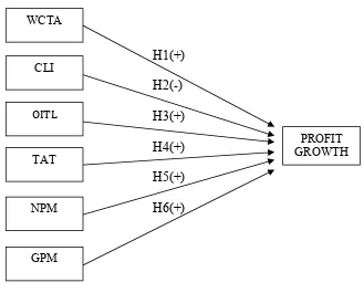
FIGURE 2.1
Theoretical Framework WCTA, CLI, OITL, TAT, NPM and GPM to Profit
Growth
WCTA become higher in the operational capital showed large companies compared to the amount of its assets (total assets). A large of working capital will facilitate the company's operations so that the company is able to pay its liabilities, thereby increasing earned profit (Reksoprayitno, 1991). Runy (2002) argues that the greater of WCTA will increase the return that would affect increase in profit growth. This is due to the efficiency of the difference between current assets and current liabilities. The influence of optimum WCTA against
profit growth is different from one industry to another (Mc Cosker, 2000). Takarini Ekawati and research results (2003) suggest that the positive effect of the WCTA is profit growth one year to come. Based on these thoughts, hypotheses can be derived as follows.
H1: WCTA Ratio effect positively to profit growth
2.4.2 Relationship Current Liability to Inventory (CLI) against Profit growth
The higher of CLI means current liabilities of the companies to finance the inventory in the warehouse be higher,so the liabilities of the company become higher either. This will be a considerable risk for the company when the company is unable to pay the liabilities at maturity, the company will also be faced with the expense of great interest, so that it will interfere with the continuity of operations of the company and the profit obtained by the company will be reduced (Reksoprayitno, 1991). This is according to research by Machfoedz (1994) and Ediningsih (2004) indicating that the CLI negatively to predict a profit growth in coming years. This proves that the company is unable to harness his liabilities to add a business expansion in order to gain an advantage. Based on these thoughts, hypotheses can be derived as follows.
H2: CLI influential negatively against profit growth
2.4.3 Relationship Operating Income to Total Liabilities (OITL) against
Profit Growth
in the company being able to pay off her liabilities. Thus the operating activities to be clear and earned income is increased, so increased profit growth. It is supported by Mahfoedz (1994) and Ediningsih (2004) that in his research shows that positive effect OITL to predict profit growth one year ahead. Based on these thoughts, hypotheses can be derived as follows.
H3: OITL influential positive Ratio of profit growth
2.4.4 Relationship a Total Assets Turnover (TAT) against Profit Growth
TAT shows efficiency of whole assets (total assets) to support the company's sales (sales) (Ang, 1997). Larger of TAT shows eficiency of company in using their companies assets to show net sales. Faster rotation of the assets of a company in order to support the net sales activities, then earned income increases so that the profits obtained will be huge (Ang, 1997). This is supported by the Ou (1990) and Asyik and Sulistyo (2000) while in their research shows TAT has positive effects with profit growth. Based on these thoughts, can be hypothesis is derived as follows.
H4: TAT influential positive effect against profit growth
2.4.5 Relationship Net Profit Margin (NPM) against Profit Growth
(Reksoprayitno, 1991). It is supported by Mahfoedz (1994), Asyik and Soelistyo (2000) and also Suwarno (2004) that in his research suggests that the positive influence of NPM significant profit growth one year ahead. Based on these thoughts, hypotheses can be derived as follows.
H5: NPM influential positive against profit growth
2.4.6 Relationship Gross Profit Margin (GPM) against Profit Growth
GPM indicates the level of refund for gross profit against net sales (Ang, 1997). GPM which increase shows that the larger of the gross profit earned by the company against net saled. This shows that the company is able to cover administrative costs, depreciation costs and also the expense of interest on the liabilities and taxes. This means the company's performance rated well and this can increase the attraction of investors to infuse equtiy in the company, so the earned income by company will be increased (Reksoprayitno, 1991). Research results by Juliana and Sulardi (2003) suggest that the positive effect of the GPM significant profit growth one year ahead. From the results of these thought the hypothesis can be derived as follows:
CHAPTER III
RESEARCH METHODS
3.1 Type of Research
The types used in this research is descriptive and verification with quantitative approach. Using type of research will be known a significant relationship between the variables examined so that conclusions that will clarify the picture of the object being studied. Type of descriptive and quantitative verification approach is a type that aims to describe the truth of the facts. Facts explain the relationship between variables was investigated by collecting data, process, analyze, and interpret data in a statistical hypotesis testing. In this study descriptive and verification are uses to test the influences of WCTA, CLI, OITL, TAT, NPM and GPM on Pofit Growth as well as to the theory by testing a hypothesis is accepted or rejected
3.2 Research Variables and Operational Definition of Variables
3.2.1 Research Variables
The research variables are the changes that have variations in value (Ferdinand, 2006). In this study, using two variables :
1. Dependent Variable
2. The Independent Variables
The independent variables are variables that affect the dependent variable, either positively or negatively, and can stand alone nature. In this study, the independent variables are WCTA, CLI, OITL, TAT, NPM, and GPM
3.2.2 Operational Definition of Variables
3.2.2.1 Dependent Variable
The dependent variable in this study is the profit growth. Profit in the study interface is Earning After Tax, it can be formulated as follows (Usman, 2003).
Δ Yit =
Where: ΔYit = profit growth in the period t
Yit = profit companies i in period t
Yit-1 = profit companies i in period t-1
3.2.2.2 Independent variable
1) Working Capital to Total Assets (WCTA)
This variable is taken from previous research by Machfoedz (1994), Takarini
WCTA =
2) Current Liabilities to Inventory (CLI)
The CLI is taken from the previous research by Machfoedz (1994) and Ediningsih (2004), Takarini and Ekawati (2003).
The CLI can be formulated as follows (Machfoedz, 1994).
CLI =
3) Operating Income to Total Liabilities (OITL)
The variable of OITL is taken from Machfoedz (1994) and Suwarno (2004).
OITL can be formulated as follows (Riyanto, 1995):
OITL=
4) Total Asset Turnover (TAT)
This variable is taken from previous research by Juliana and Sulardi (2003), Suwarno (2004) and Meythi (2005). TAT can be formulated as follows (Ang, 1997).
5) Net Profit Margin (NPM)
NPM shows company's ability to generate revenue againts his net sales (Riyanto, 1995). This variable is taken from previous research by Juliana and Sulardi (2003).
NPM can be formulated as follows (Ang, 1997).
NPM
=
6) Gross Profit Margin (GPM)
GPM is one of the ratios which indicate the level of refund for gross profit against net sales (Ang, 1997). This variable is taken based on the previous research by Juliana and Sulardi (2003).
GPM can be formulated as follows (Ang, 1997)
Table 3.1
Operational Definition
No Variable Definition Scale Formulation Literature
1 Working Capital result from net sales minus the cost of goods sold and operating expenses) to the sales by the number of assets
Ratio Ang, 1997
5 Net Profit Margin
comparison between the net profit after tax on total sales.
Ratio Ang, 1997
CA: Current Assets, CL: Current Liabilities,TA: Total Assets, I : Inventory OPBIT : Operating Profit before Interestand Taxes, L : Liabilities
3.3 Population and Sample
3.3.1 Population
The population used for this research is the entire manufacturing company listed in IDX since 2008 to 2012 which includes 123 manufacturing companies. Based on previous research which the researches analyze the financial ratio at a manufacturing company listed on the IDX in generally. In previous researches used the pre-2008 period, while this study used the time period from 2008 -2012, more updates in the years of observation. In this research choosing the manufacturing company because the manufacturing company as the number of public companies that are included in the manufacturing sector looks to dominate listed in IDX.
3.3.2 Samples
The selection of the sample was determined by purposive sampling with purpose to get a representative sample in accordance with the specified criteria. The criteria to be selected into the sample are:
1. Manufacturing companies registered in IDX during the research period (2008 to 2012).
2. Manufacturing company which published the financial statements during the research period (2008 to 2012).
3.4 Data
3.4.1 Types and Sources of Data
Type of data used in this research is quantitative data, if a series of observations (measurements) can be expressed in numerical values, so the collection of numerical values itself on the observation called quantitative data (Lincolin Arsyad, 1997). The sources of data from secondary data that is in the form of annual financial statements of listed manufacturing companies in IDX with year-end bookkeeping on December 31 2008, 2009, 2010, 2011 and 2012. The data source can be obtained from the Indonesian Capital Market Directory (ICMD) and IDX official website.
3.4.2 Methods of collecting Data
The Data in this study were obtained by using the method of documentation i.e. data collection by way of collecting secondary data from the financial statements that have been published on the IDX. The financial statements of companies listed in ICMD 2008, ICMD 2009, ICMD 2010, ICMD 2011, ICMD 2012 and also from official website of IDX.
3.5 Classic Assumption Test
3.5.1 Normality Test
Smirnov test (Ghozali, 2005). This normality test can be done through graph analysis and statistical analysis.
1. Graph analysis
One of the easiest ways to see residual normality is by looking at the histogram graph that compares between the observation data with the normal approach to the distribution. However, just by looking at the histogram, it can be confusing, especially for a small number of samples. Another method that can be used is to look at normal probability plot that compares the cumulative distribution from normal distribution. The basis of decision-making analysis from normal probability plot is as follows:
a. If the data is spread around the diagonal line and follow the direction of a diagonal line indicates the pattern of a normal distribution, so regression models meet the assumption of normality.
b. If the data spread away from the diagonal line and or do not follow the direction of a diagonal line pattern does not show a normal distribution, regression model does not fulfill the assumption of normality.
2. Statistical Analysis
To detect the normality of data can be done through statistical analysis which can be seen through the Kolmogorov-Smirnov test (K-S).
Basic of decision making in the K-S test is as follows:
a. If the probability of value Z the K-S test statistically significant so Ho is rejected, which means a distributed data is not normally.
Guidelines for decision making are as follows:
a) Value sig. or significance or probability value < 0.05 distribution is not normal.
b) The value of sign. Or significance or probability value > 0.05 distribution is normal.
3.5.2 Multicollinearity Test
According to Ghozali (2005), this test is used to determine whether there is a correlation between independent variables in the regression model. A good regression model should not have correlation between independent variables. If there is a correlation between independent variables, these variables are not orthogonal. Orthogonal variable is the independent variable that value of a correlation between fellow independent variables is zero. To detect there is or no multicollinearity in regression models can be seen from the tolerance valueor the variance inflation factor(VIF). See as the basis it can be concluded:
1. If the tolerance value > 0.1 VIF value < 10, it can be concluded that there is no multicollinearity between independent variables in the regression model.
3.5.3 Autocorrelation Test
Autocorrelation test aimed to test whether linear regression model has correlation between fault disturber in the t period with fault disturber in the period t-1 (earlier). If there is a correlation, so there is a problem of autocorrelation. Autocorrelation arises due to successive observation at all times in relation to another. This problem occurs because the residual (fault disturber) is not free from one observation to another observation, usually found in time series data. The consequences of the presence of autocorrelation in regression model is a variance sample can't describe the population variance, so the result of regression model can’t be used to estimate the value of dependent variable in value of certain independent (Ghozali, 2005)
3.5.4 Heterocedasticity Test
This test aims to test whether the regression model occured inequality variance from residual one observation to other observation. If the residual variance from one observation to another observation remains, it is called Homocedasticity and if different called Heterocedasticity. Good of regression Model is homocedasticity or heterocedasticity does not occur. To detect the presence of heterocedasticity is done by looking at the plot graph between the value prediction variable (ZPRED) and the residual (SRESID). The basis of analysis:
1. If there is a particular pattern, such as points that form a specific pattern, a regular (wavy, widened, then narrowed), indicates there has been a heterocedasticity.
2. If there is no specific pattern and also the points spread above and below zero on the Y axis, then it doesn't occured heterocedasticity, and indicates there has been a heterocedasticity. Analysis with plots graph has significant weaknesses because of the number of observation affects the result of ploting. Fewer the number of observations, will more difficult to interpret the results of plot graph.
3.6 Analysis Techniques
The study uses Multiple Regression Analysis. Multiple linear regression analysis was used to examine the influence of financial ratios to profit growth.
The Model in this research are:
Where : Yt = Profit Growth
a = Constant coefficient
b = Regression coefficient of each variable
X1 = WCTA
X2 = CLI
X3 = OITL
X4 = TAT
X5 = NPM
X6 = GPM
e = Error Coefficient (disturbing variable)
3.7 Hypothesis Testing
After doing normality test and the classical assumptions test, the next step is doing the testing of 1st hypothesis (H1) up to the 6th hypothesis (H6). Test of
significance is a procedure where the results of the sample used to test the truth of a hypothesis (Gujarati, 1999). Analysis tools use t-test and Coefficients determinantion (R2). Statistical calculation called statistically significant if the test
values the statistics are in critical areas (area where Ho is rejected). Instead, it is called not significant value when the statistic tests are in the area where the Ho is accepted.
3.7.1 Coefficient Determination (R2)
Coefficient of determination (R2) essentially measures how much the
the ability of independent variables in explaining the dependent variable, is limited. Instead, the value of R2 that approximates the one signifying the
independent variables provide almost all of the information required by the dependent variable (Ghozali, 2005). The value used is the adjusted R2 because
independent variables used in this study more than two pieces.
3.7.2 F Test Statistic
F statistical test basically shows whether all the independent variables were entered independently or jointly influence on the dependent variable or bound (Ghozali, 2006).
How to test F are as follows:
1. Comparing the results chance to make mistake (level of significance) appears, with the advent of the incidence rate of chance (probability) that was set at 5% or 0.05 on the output, to make a decision to reject or accept the null hypothesis (Ho):
a. If the significance of> 0.05 then the decision is to accept Ho and reject Ha
b. If the significance of <0.05 then the decision is to reject Ho and accept Ha
2. Comparing the value of the F statistic is calculated with F statistics value table:
F-test formula is (Priyatno, 2008):
= (1 − )
( − 1 − )
Where:
= squared multiple correlation coefficient
n = Total sample
k = Total independent variable
3.7.3 T test Statistic
T statistical test basically shows how far the influence of the explanatory variables / independent individual in explaining the variation in the dependent variable (Ghozali, 2006). How to perform a t-test is as follows:
1. Comparing the results much chance it false (level of significance) appears, with the advent of the incidence rate of chance (probability) that was set at 5% or 0.05 on the output, to make a decision to reject or accept the null hypothesis (Ho):
a. If the significance of > 0.05 then the decision is to accept Ho and reject Ha
2. Comparing the value of t statistics calculated by the value of t statistics table:
a. If the statistical value t test < t table, then Ho is accepted b. If the statistical value t test > t table, then Ho is rejected
T test formula is (Priyatno, 2008):
to =Sbb
Where:
To = t arithmetic
Bi = coefficient regression
CHAPTER IV
RESULTS AND DISCUSSION
`
4.1. General Overview and Descriptive Data of Research Object
4.1.1. Research Object Overview
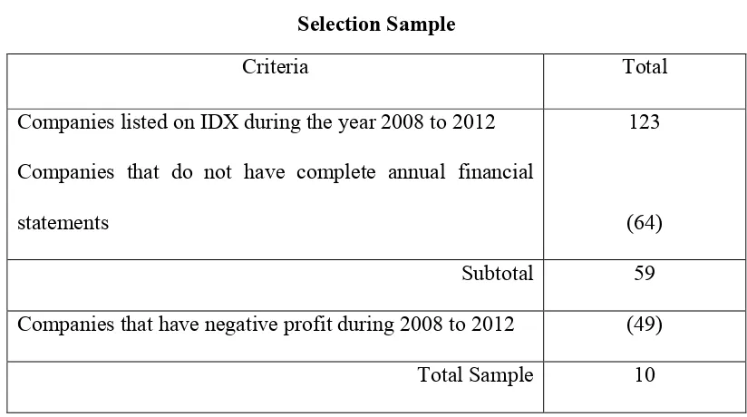
As the sampling criteria, this research used a sample of manufacturing companies during the period 2008 to 2012 issuing a annual financial report with positive profit information. Obtained 10 companies sampled which is then used as a source of data for analysis. The sample selection process is presented in Table 4.1 below.
Table 4.1
Selection Sample
Criteria Total
Companies listed on IDX during the year 2008 to 2012 Companies that do not have complete annual financial statements
123
(64)
Subtotal 59
Companies that have negative profit during 2008 to 2012 (49)
Total Sample 10
Based on Table above companies that do not have complete annual financial statements as many as 64. AQUA company as example, in a 2008 reported financial statements then in 2009 did not report financial statements but in 2010 reported financial statements. Companies that have negative profit during 2008 to 2012 as many as 49 companies.
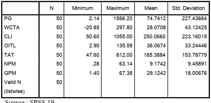
4.1.2 Descriptive Data
This research uses the data in the form of pooled cross sectional. The research was conducted in 2008 to 2012 with a sample of 10 manufacturing companies, it is a pooled cross-sectional obtained a number of 10 companies x 5 years = 50 observations. Independent variables used in this study is WCTA, CLI, OITL, TAT, NPM and GPM, while the dependent variable is profit growth. Data for variables WCTA, CLI, OITL, TAT, NPM, GPM and profit growth obtained through calculations based on annual financial report prepared obtained from IDX.
Table 4.2
Description of Research variables beginning observations (n=50)
Descriptive Statistics
N Minimum Maximum Mean Std. Deviation
PG 50 2.14 1566.20 74.7412 227.43664
WCTA 50 -20.85 297.80 28.0708 43.12425
CLI 50 50.60 1055.00 250.0660 223.16015
OITL 50 2.90 135.59 36.0674 33.24446
TAT 50 47.60 812.00 185.3884 153.78779
NPM 50 .28 63.14 9.1742 9.45891
GPM 50 1.40 67.38 29.1242 18.00676
Valid N
(listwise)
50
Source : SPSS 19
Based on calculations in Table 4.2, it appears that from the 10 companies with 50 observations, the mean profit growth during the observation period (2008 to 2012) of 74.7412 with δ at 227.43664; whereby these results indicate that the value ofδ> mean profit growth, as well as the minimum value that is smaller than the mean (2.14) and the maximum value is greater than the mean (1566.20).
4.2. Classic Assumption Test
Classic Assumption test is used to test, whether the regression model used in this research were tested or not feasible. Classical assumption test is used to ensure that multicollinearity, autocorrelation, and heteroscedasticity are not included in the model used and the resulting data were normally distributed. If the overall requirements are met, means that the model had decent analysis used (Gujarati, 1999). Deviance test classic assumptions, can be described as follows.
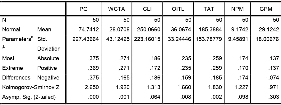
4.2.1. Normality Test
Table 4.3
Result of Normality Test (Beginning Data) (n=50)
One-Sample Kolmogorov-Smirnov Test
PG WCTA CLI OITL TAT NPM GPM
N 50 50 50 50 50 50 50
Normal
Parametersa
,b
Mean 74.7412 28.0708 250.0660 36.0674 185.3884 9.1742 29.1242
Std.
Deviation
227.43664 43.12425 223.16015 33.24446 153.78779 9.45891 18.00676
Most
Extreme
Differences
Absolute .375 .271 .186 .235 .259 .174 .137
Positive .369 .271 .172 .235 .259 .170 .137
Negative -.375 -.165 -.186 -.159 -.185 -.174 -.074
Kolmogorov-Smirnov Z 2.650 1.920 1.313 1.660 1.830 1.227 .971
Asymp. Sig. (2-tailed) .000 .001 .064 .008 .002 .098 .303
a. Test distribution is Normal.
b. Calculated from data.
Source : SPSS 19
Table 4.4
Normality Test (Data without outlier) (n=31)
One-Sample Kolmogorov-Smirnov Test
PG WCTA CLI OITL TAT NPM GPM
N 31 31 31 31 31 31 31
Normal
Parametersa,b
Mean 29.3845 24.6732 183.1177 34.9458 132.6290 9.2642 35.3952
Std.
Deviation
28.58992 19.06209 124.90375 22.12829 56.35185 4.42236 16.32708
Most
Extreme
Differences
Absolute .222 .078 .205 .242 .233 .099 .150
Positive .222 .078 .205 .242 .233 .084 .150
Negative -.175 -.078 -.144 -.123 -.116 -.099 -.120
Kolmogorov-Smirnov Z 1.238 .434 1.142 1.345 1.295 .552 .837
Asymp. Sig. (2-tailed) .093 .992 .147 .054 .070 .920 .485
a. Test distribution is Normal.
b. Calculated from data.
Souce : SPSS 19
Figure 4.1 Graphic Plot
Source : The research data wereanalyzed using SPSS 19
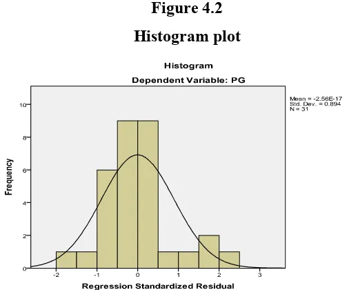
From Figure 4.1, it is seen that the pointsare variable around the line Y = X or spread around the diagonal line and its distribution following the direction of the diagonal line, this indicates that the data was normally distributed. While this research histogram shown in Figure 4.2 below.
Figure 4.2 Histogram plot
From Figure 4.2, it is seen that the histogram chart gives a close to normal distribution patterns.
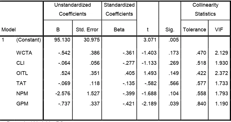
4.2.2 Multicollinearity Test
Multicollinearity test is intended to determine whether there is a perfect intercorrelations between the independent variables used in this research. This test is performed with Tolerance Value and Variance Inflation Factor (VIF). To avoid multicollinearity, Tolerance limit Value> 0.1 and VIF <10. The multicollinearity test results in this research can be seen in Table 4.5.
Table 4.5
B Std. Error Beta Tolerance VIF
1 (Constant) 95.130 30.975 3.071 .005
WCTA -.542 .386 -.361 -1.403 .173 .470 2.129
CLI -.064 .056 -.277 -1.133 .269 .518 1.930
OITL .524 .351 .405 1.493 .149 .422 2.372
TAT -.069 .118 -.135 -.582 .566 .577 1.733
NPM -2.576 1.527 -.399 -1.688 .104 .558 1.793
GPM -.737 .337 -.421 -2.189 .039 .840 1.190
a. Dependent Variable: PG
Based on Table 4.5, the tolerance values > 0.1 and VIF < 10, so it can be concluded that all six independent variables was no multicollinearity correlation and can be used to influence the profit growth during the observation period.
4.2.3 Autocorrelation Test
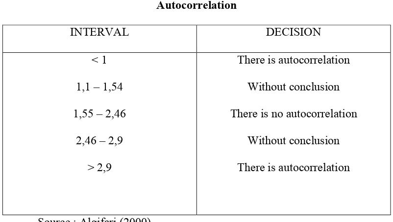
Autocorrelation indicates a correlation between the disturber error in period t with error in period t-1. Consequently, the variation of the sample can’t describe population variation. Further consequence, the resulting regression model can’t be used to assess the value of the dependent variable from its independent variable. To find out the availability of autocorrelation in a regression model, performed Durbin-Watson test (DW) under the conditions presented in Table 4.6 as follows (Algifari, 2000).
Table 4.6
Autocorrelation
INTERVAL DECISION
< 1 1,1 – 1,54 1,55 – 2,46
2,46 – 2,9 > 2,9
There is autocorrelation Without conclusion There is no autocorrelation
Without conclusion There is autocorrelation
On the this research data, a score of DW is 2,367 as shown in Table 4.7.
Table 4.7
Autocorrelation Test Result
Model Summaryb
Model R
R
Square Adjusted R Square
Std. Error of the
Estimate Durbin-Watson
1 .503a .253 .067 27.61767 2.367
a. Predictors: (Constant), GPM, TAT, CLI, NPM, WCTA, OITL
b. Dependent Variable: PG
Source : SPSS 19
Based on calculations using SPSS 19 in Table 4.7 DW value is between 1.55 to 2.46, so it can be concluded that there is no autocorrelation in the regression equation in this research.
4.2.4 Heterocedasticity test
Figure 4.3 Scatter Plot Diagram
Source : The research data were analyzed using SPSS 19
By looking at the scatterplot graphs, dots randomly spread, and spread both above and below the 0 on the y-axis it can be concluded that there are no symptoms of heteroscedasticity in regression models were used.
4.3 Multiple Regression Analysis
4.3.1 Coefficient of Determination (R2)
The coefficient of determination (R2) was essentially measure how far the ability of the model in explaining the dependent variable. Small value of R2which means the ability of the independent variables in explaining the dependent variable is limited. In contrast, the value of R2 close to unity indicates the independent variables provide almost all the information required by the dependent variable (Ghozali, 2005). The value used is the adjusted R2 for the independent variables used in this study is more than two pieces. The adjusted R2 value of the calculation using SPSS 19 is shown in Table 4.8.
Table 4.8 R2Value
Model Summaryb
Model R R Square Adjusted R Square
Std. Error of the
Estimate
1 .503a .253 .067 27.61767
Source : SPSS 19
From the calculation results of the influence of the independent variable on the dependent variable that can be explained by the model of this equation is equal to 6.7% and the rest equal 93.3% is influenced by other factors that are not included in the regression model.
4.3.2 F test Statistic
earnings growth. It can proof of the value of F smaller size of 0.001 significance level that is as large as 0.05 as shown in table 4.9 as follows :
Table 4.9
F test Regression Result
ANOVAb
Model Sum of Squares df Mean Square F Sig.
1 Regression 6215.852 6 1035.975 1.358 .001a
Residual 18305.655 24 762.736
Total 24521.507 30
a. Predictors: (Constant), GPM, TAT, CLI, NPM, WCTA, OITL
b. Dependent Variable: PG
Source : SPSS 19
4.3.3 t Test Statistic
This test aims to determine whether or not the influence of the independent variable on the dependent variable (partially) with regard to other independent variables constant. The test is performed by comparing the significance value indicated by Sig t of t in Table 4.10 with a significance level taken, in this case 0.05. If the Sig value of t <0.05 then the independent variables affect the dependent variable.
1 (Constant) 95.130 30.975 3.071 .005
WCTA -.542 .386 -.361 -1.403 .173
CLI -.064 .056 -.277 -1.133 .269
OITL .524 .351 .405 1.493 .149
TAT -.069 .118 -.135 -.582 .566
NPM -2.576 1.527 -.399 -1.688 .104
GPM -.737 .337 -.421 -2.189 .039
So based on Analysis technique which the formula is:
Yt = a + b1X1 + b2 X2 + b3 X3 + b4 X4 + b5X5 + b6X6 + e
We can make the profit growth formula as follows :
∆PROFIT = 95,130 - 0,542 WCTA - 0,064 CLI + 0,524 OITL
– 0,069 TAT - 2,576 NPM – 0,737 GPM + e
Based on calculations using SPSS 19, it can be seen that only one independent variable is the variable GPM which significantly affect the dependent variable is profit growth, with a significance level of 0.039 while the variable WCTA, CLI, OITL, TAT, NPM has no significant effect on profit growth. This is because the value for the variable t sig WCTA, CLI, OITL, TAT and NPM respectively 0.173; 0.269; 0.149; 0.566; and 0.104, which means greater than the significance level of 0.05.
4.4 Hyphotesis Testing
4.4.1 Hyphotesis 1 (H1)