*Corresponding author. Tel.: 34-924-289300-ext.9183; fax: 34-924-272509.
E-mail address:[email protected] (L.R. Murillo-Zamorano).
The use of parametric and non-parametric frontier methods to
measure the productive e$ciency in the industrial sector:
A comparative study
Luis R. Murillo-Zamorano
!
,
*
, Juan A. Vega-Cervera
"
!Department of Economics, University of Extremadura, Avda. de Elvas s/n, 06071 Badajoz, Spain
"Department of Economics and Related Studies, Universitry of York, Heslington, Y01 5DD, UK Received 26 May 1999; accepted 27 January 2000
Abstract
Parametric frontier models and non-parametric methods have monopolised the recent literature on productive
e$ciency measurement. Empirical applications have usually dealt with either one or the other group of techniques. This
paper applies a range of both types of approaches to an industrial organisation setup. The joint use can improve the
accuracy of both, although some methodological di$culties can arise. The robustness of di!erent methods in ranking
productive units allows us to make a comparative analysis of them. Empirical results concern productive and market
demand structure, returns-to-scale, and productive ine$ciency sources. The techniques are illustrated using data from
the US electric power industry. ( 2001 Elsevier Science B.V. All rights reserved.
Keywords: Productive e$ciency; Parametric frontiers; DEA; Industrial sector
1. Introduction
Since such authors as Debreu [1], Koopmans [2] or Farrell [3] introduced the analysis of e$-ciency in the economic literature, there has been a wide-ranging collection of papers and articles devoted to the measurement of productive e$cien-cy. There has always been a close link between the measurement of e$ciency and the use of frontier functions. Di!erent techniques have been utilised to either calculate or estimate these frontier func-tions. In this study we go through their joint use as
well as their application to an industrial organisa-tion framework.
Most of the papers related to the measurement of productive e$ciency have based their analysis either on parametric or on non-parametric methods. The choice of estimation method has been an issue of debate, with some researchers preferring the parametric approach (e.g. [4]) and others the non-parametric approach (e.g. [5]). The main disadvantage of non-parametric approaches is their deterministic nature. Data envelopment analysis (DEA), for instance, does not distinguish between technical ine$ciency and statistical noise e!ects. On the other hand, parametric frontier func-tions require the de"nition of a speci"c functional form for the technology and for the ine$ciency error term. The functional form requirement
1Panel data techniques can also improve the accuracy of the parametric approach to the measurement of productive e$ cien-cy. For a detailed comparative analysis of these techniques, see [16].
2As it is pointed out for one anonymous referee what is given in relations (1)}(7) is not new but it constitutes the theoretical framework used in the empirical application.
3Gabrielsen [17]. causes both speci"cation and estimation problems.
Obviously, it would be desirable to introduce more #exibility into the parametric frontiers, as well as more thoroughly investigate the non-parametric and stochastic methodologies (e.g. [6]). In our opinion neither approach seems to be strictly pre-ferable. Instead, we think that the joint use of the two groups of techniques can improve the accuracy with which they measure productive e$ciency. Fol-lowing recent literature (e.g. [7]), the aim of this paper is to provide the framework for the joint use of them. By doing so, one hopes to avoid the weaknesses inherent, and bene"t from the strong aspect of each to the two methods, although in general this is not a very easy job to be done.
The set of data utilised is partially taken from the one used in [8]. The paper of Lee examines the issue of vertical integration in the US electricity industry in 1990. Three stages}generation, trans-mission, and distribution } are analysed in his study. Our study focuses just on the generation stage and therefore no comparative analysis with Lee's study is made.
We organise the paper as follows. Section 2 introduces the techniques used to measure the productive e$ciency. Section 3 presents the data set and discusses the results. Finally, Section 4 pres-ents the conclusions.
2. Methods
2.1. The parametric approach
The parametric approach is naturally subdivided into deterministic and stochastic models. Deter-ministic models envelope all the observations, identifying the distance between the observed pro-duction and the maximum propro-duction, de"ned by the frontier and the available technology, as tech-nical ine$ciency. On the other hand, stochastic approaches permit one to distinguish between technical e$ciency and statistical noise.
The measurement of productive e$ciency by means of parametric techniques requires the speci-"cation of a particular frontier function. The Dual-ity theory suggests the use of cost functions to de"ne the production structure. Nerlove [9]
introduced the use of cost functions in the analysis of regulated industries with his application to elec-tric sector. The output produced by "rms under a regulated environment, as well as the prices they pay for factors in competitive markets, can be con-sidered to be exogenous. This fact makes the choice of cost functions attractive.
Every cost function implies a set of derived demand equations. Christensen and Greene [10] argued that the joint use of a cost function and a set of cost share equations as a multivariate regression system provides better estimates of the production structure than those derived from single-equation procedures. The dual frontier econometric ap-proach has also evolved from the estimation of single-cost functions (e.g. [11]) to multiple-equation systems (e.g. [12,13]). However, some serious estima-tion and speci"caestima-tion problems "rst noted by Greene [14], and Nadiri and Schankerman [15], still remain unsolved.1Because of this, the techno-logy form "nally adopted was a Cobb}Douglas production function and the frontier production function speci"ed can be represented as
log>
composed error term wherev
i represents
random-ness (or statistical noise) andu
irepresents technical
ine$ciency. In the deterministic approach v
i will
equal zero.
4This was"rst noted by Richmond [18].
5Aigner et al. [19], Meeusen and van den Broeck [20], and Battese and Corra [21].
since that estimation procedure is robust to non-normality.4If the estimated intercept term is cor-rected by shifting it upward until no residual is positive and at least one is zero, we also get a consistent estimator of the intercept term.
Let us assume the following model:
y
and individual technical e$ciency will be
¹E
i"e~k
(
iCOLS.
Unlike the deterministic approach, the stochastic frontier models5 capture the e!ects of exogenous shocks beyond the control of the analysed units. Errors in the observations and in the measurement of output are also taken into account in this kind of models.
For the Cobb}Douglas case, the stochastic fron-tier can be represented by Eq. (1). The error repres-enting statistical noise is assumed to be identical independent and identically distributed. With re-spect to the one-sided (ine$ciency) error, a number of distributions have been assumed in the literature, the most frequently used ones being half-normal (SFN), truncated from below at zero (SFT) and exponential (SFE). If the two error terms are as-sumed independent of each other and of the input variables and some of the previous distributions are used, then the likelihood functions can be de"ned and maximum likelihood estimates can be deter-mined.
Once the model has been estimated by using maximum likelihood techniques, we obtain a"tted value for the composed error term v
i!ui. For
e$ciency measurement, we need to separate these
two error terms. Jondrow et al. [22] proposed one way to do it. They developed an explicit formula for the expected value of u
i conditional on the
com-posed error term (E(u
where /(.) is the density of the standard normal distribution andU(.) the cumulative density func-tion.
Greene [23] shows that the conditional technical ine$ciencies for the truncated model are obtained by replacing e
ij/p in the expression for the
half-normal case, with
Finally, individual (conditioned) technical e$cien-cy scores will be
¹E
i"e~E*ui@ei+.
2.2. The non-parametric approach
6See [24]. A more detailed analysis of alternative formula-tions can be found in [25,26].
7According to an output-oriented model formulation. 8Whether those variable returns to scale represent increasing or decreasing returns to scale will depend on the relationships among technical e$ciency scores calculated under constant, variable or non-increasing returns to scale.
a peer group consisting of a linear combination of e$cient DMUs. For each unit not located on the e$cient frontier, we de"ne a vectork6"(k1,2,kn)
where eachk
j represents the weight of each DMU
within that peer group. The DEA calculations are designed to maximise the relative e$ciency score of each unit, subject to the constraint that the set of weights obtained in this manner for each DMU must also be feasible for all the others included in the sample. That e$ciency score can be calculated by means of the following mathematical program-ming formulation6where technical e$ciency scores will be determined by the optimum t. Constant (TEc) and variable returns to scale (TEv) formula-tions are described.
Operation research techniques usually use the dual of the above problem in order to calculate the e$ciency scores. Such a dual formulation can be obtained as the minimum of a ratio of weighted inputs to weighted outputs subject to the constraint that the similar ratios for every DMU be greater than or equal to unity. For an output-oriented
model, the dual formulation is
Min
randzi are the variable weights that solve
this maximisation problem and >
rj and Xij the
outputs and inputs attached to each DMU. A unit will be e$cient if and only if this ratio equals one, otherwise it will be considered as relatively ine$cient.
DEA can also be used to calculate scale e$cien-cy. Total technical e$ciency is de"ned7in terms of equiproportional increases in outputs that the"rm could achieve while consuming the same quantities of its inputs if it were to operate on the constant returns to scale (CRS) production frontier. Pure technical e$ciency measures the increase in out-puts that the"rm could achieve if it were to use the variable returns to scale (VRS) technology. Finally, scale e$ciency would be calculated as the ratio of total technical e$ciency to pure technical e$cien-cy. If scale e$ciency equals one, the"rm is operat-ing at CRS, otherwise it would be characterised by VRS.8
3. Data and results
Table 1
Main descriptive statistics of variables used in the study
Variable Mean Max. Min. Standard
deviation
Total output 15.582 70.517 1.678 1.568E#10
Total capital 94.914 409.673 9.367 91.747
Total labour 4.993 24.607 440 5.198
Total fuel 1.324E#10 4.750E#11 7.001E#09 1.111E#11
% Ksteam! 0.7674 0.9999 0.084 0.2192
% Knuclear! 0.1120 0.6754 0 0.1762
% Khydroelectric! 0.0422 0.3256 0 0.0757
% Kother GE! 0.0783 0.9150 0 0.1280
% Ocommercial" 0.2664 0.6421 0.037 0.0987
% Oindustrial" 0.3485 0.5533 0.1052 0.0774
% Oresidential" 0.3850 0.8113 0.063 0.1272
!Represents the percentage of capital stock levels attached to steam, nuclear, hydroelectric and other power-generating equipment assets.
"Allocation of total MWh to commercial, industrial and residential demand categories.
9A major description of the set of data and variables used in this study can be found in [8].
10Actually, this hypothesis was strongly accepted when we imposed the constraint (b
1)#(b2)#(b3)"1 to the initially unrestricted model. The estimation procedure was made using Limdep 7.0.
di!erent measures of e$ciency and compare public versus private performance of electric utilities. Hjal-marsson and Veiderpass [30] study the local retail distribution of electricity in Sweden in 1985. They apply di!erent versions of the DEA model to 329 "rms. Using DEA techniques and OLS analysis, Pollit [31] examines the cost e$ciency in 129 elec-tricity transmission and 145 elecelec-tricity distribution systems in 1990. Lastly, Ray and Mukerjee [32] perform a comparative analysis of parametric fron-tier dual cost functions and non-parametric tech-niques applied to the data set used previously [11]. The data set used in the present empirical application corresponds to a sample of 70 US (in-vestor-owned) electric utility"rms in 1990. These "rms are approximately evenly spread across the United States. Table 1 provides descriptive statis-tics for each of the variables used in this study.
The capital stock variable is constructed for four di!erent asset classes: steam, nuclear, hydroelectric and other power-generating equipment. In any case, steam technology accounts for most of the electricity generated by the companies analysed in this study. The labour variable indicates the num-ber of workers of each"rm. There are four main categories of fuel: coal, oil, natural gas, and nuclear. BTU equivalents are used to aggregate di!erent types of fuels over all plants belonging to one"rm. The fuel variable is the measure in millions of BTUs
used in generation of electricity. Finally, total output is indicated in megawatts hours (MWh).9
3.1. Ezciency scores
With respect to the parametric frontiers the estimated parameters of the deterministic and stochastic production functions are given in Table 2. These results come from estimating Eq. (1) by means of COLS and MLE, where i"1,2, 70
indicates the "rms, >
i the output, X1,i"Ki the
capital stock,X
2,i"¸ithe number of workers, and
X
3,i"Fi the fuel;b1,b2andb3are the elasticities
Table 2
Estimated parameters of deterministic and stochastic produc-tion frontiers. (t-test statistics appear in parentheses)
COLS SFN SFT SFE
Intercept (a) 10.819! 11.786 11.145 10.951 (10.014) (15.870) (13.886) (14.453) Capital (b1) 0.1392 0.1340 0.1066 0.1391
(2.414) (1.893) (1.330) (2.270) Labour (b2) 0.6441 0.6745 0.6713 0.6441
(10.539) (10.865) (10.084) (11.485) Fuel (b
3) (3.474)0.2174 (3.954)0.1794 (4.705)0.2170 (4.847)0.2174
R2 0.9506
F 423.529
Log-Lik. 10.1631 11.3880 11.1224 11.8625
pu/pv 1.7239 2.2007
(1.897) (1.405)
p2u 0.0621 0.0995 0.0176
p2v 0.0209 0.0205 0.0261
(b1)#(b2)#(b3)" 1.0007 0.9879 0.9949 1.0006
M0.9756N [0.3570] [0.1421] [0.0230]
!If the estimated intercept term is corrected by shifting it upward until no residual is positive and at least one is zero, we will get a consistent estimator of the intercept term. In our case this consistent intercept is 11.349.
"CRS hypothesis test:.M}N:Probability associated with an F
-Test (1.66). [}]: Signi"cance level in a Wald Test-s2(1).
11According to Klein's rule of thumb, multicollinearity is a problem if maxR2j'R2whereR2j is theR2statistic from the OLS estimation of the auxiliary regression of thejth regressor on the other regressor and the intercept term. Several auxiliary regressions were estimated and in all of them this condition was found. Moreover, when we checked the functional form
speci-"cation of the model, applying a RESET}Test, the Cobb} Doug-las technology turned out to be well speci"ed.
Table 3
Technical e$ciency averages Method Average
e$ciency!
Max. Min. Standard deviation
Number of e$cient units
COLS 60.09 1 28.95 0.123 1
SFN 82.61 94.86 49.72 0.086 0
SFT 87.77 96.31 54.33 0.073 0
SFE 87.64 95.93 49.66 0.080 0
DEAc 73.32 100 33.3 14.77 6
DEAv 78.71 100 6.9 19.39 16
!The average e$ciency measures of COLS, SFN, SFT, and SFE were estimated under the null hypothesis of constant re-turns to scale.
12The individual e$ciency scores generated by each method are available from the authors upon request.
13The one with the largest positive OLS residual. estimation of full translog functions can be
hampered by an important problem of multicol-linearity.11
Each of the stochastic speci"cations yields sim-ilar estimates for the partial elasticities of output with respect to capital, labour and fuel. This result seems to con"rm the robustness of the technology
and distribution hypotheses assumed in the speci-"cation of the model.
Table 3 reports the average technical e$ciency measures for each of the models explained in the Methods section.12
As the theory advances, the average e$ciency scores of parametric deterministic techniques are lower than the ones estimated through stochastic frontier approaches. Given that COLS is a not stochastic procedure, noise is also reported as ine$ciency.
COLS shifts all the residuals down to non-posit-ive values and only one "rm of the sample is estimated as e$cient.13 With respect to the DEA approaches, given that the constraint set is less restrictive under CRS than under VRS, lower e$-ciency scores are reported for the former case. In our example, DEAc presents an average level of technical e$ciency of 73.32% while DEAv e$cien-cy average is 78.71%. For the same reason, fewer units are found to be e$cient under CRS than under VRS.
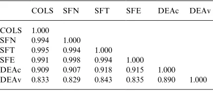
Table 4
Spearman correlation coe$cients among alternative e$ciency measures!
COLS SFN SFT SFE DEAc DEAv
COLS 1.000 SFN 0.994 1.000 SFT 0.995 0.994 1.000 SFE 0.991 0.998 0.994 1.000 DEAc 0.909 0.907 0.918 0.915 1.000 DEAv 0.833 0.829 0.843 0.835 0.890 1.000
!All the correlation coe$cients among di!erent methods are signi"cant at the 0.01 level (2-tailed).
14Spearman's correlation coe$cients were calculated using the SPSS 8.0 package.
in any case, the choice of distribution assumptions does not seem to have a signi"cant e!ect on the values of the e$ciency estimates.
Stochastic frontier models' estimates of p2 v and
p2
u provide us with a measure for the relative
importance of statistical noise and ine$ciency in the estimation of frontier production functions. The variance of the composed error termp2
e is de"ned
as the sum of the variance of the ine$ciency error term p2u and the variance of the statistical noise termp2v. Therefore, the (%) participation of each of these components } u and v } in the aggregated error term e can be determined by means of the relationships %
u"p2u/(p2u#p2v) and %v"
p2
v/(p2u#p2v). According to the information in Table
2, noise represents 59.72% of total variance in the exponential model. In the half-normal and in the truncated cases, these proportions are lower, 25.18% and 17.08%, respectively, but still broadly indicative of the importance of noise in the estima-tion of these models. Therefore, the fact that deter-ministic models do take noise into account seems to be quite important in our illustrative application. Especially noticeable is the COLS procedure where the average level of technical e$ciency is around 60%. These models therefore su!er from both drawbacks: the problems of a rigid speci"ca-tion associated to their parametric nature, and the shortcoming of not distinguishing between ine$ciency and noise given their deterministic structure.
3.2. Robustness
Having analysed the e$ciency scores, we explore the consistency of the above models in ranking the 70 electric utilities that make up our sample. We are interested in the robustness of the relative position of each electric utility to the use of di!erent methods, rather than in the average levels of tech-nical e$ciency found. Table 4 presents pairwise Spearman rank correlation coe$cients of the e$ciency scores yielded by the six methods used in our analysis.14
These results show that parametric models are extremely consistent in ranking the units. Their pairwaise correlation coe$cients are not less than 99%. The correlation is also high between paramet-ric techniques and DEAc. On the other hand, cor-relation coe$cients between DEAv and both the econometric approaches and DEAc are not so high. They are around 83% for the group of parametric techniques and 89% for the DEAc model. All para-metric approaches were also estimated by imposing the CRS constraint. It seems that the choice of parametric or non-parametric techniques, deter-ministic or stochastic approaches, or between dif-ferent distribution assumptions within stochastic techniques is irrelevant if one is interested in ranking electric utilities according to their indi-vidual e$ciency scores. Only the VRS speci"cation leads to certain di!erences in those rankings, al-though such di!erences are not so large as to stop these rankings still being comparable with the others.
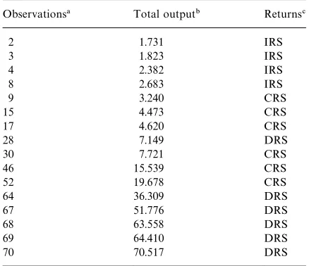
Table 5
Returns to scale ofe$cient units
Observations! Total output" Returns#
2 1.731 IRS
3 1.823 IRS
4 2.382 IRS
8 2.683 IRS
9 3.240 CRS
15 4.473 CRS
17 4.620 CRS
28 7.149 DRS
30 7.721 CRS
46 15.539 CRS
52 19.678 CRS
64 36.309 DRS
67 51.776 DRS
68 63.558 DRS
69 64.410 DRS
70 70.517 DRS
!Ordered by output produced.
"MWh.
#IRS: increasing returns to scale, CRS: constant returns to scale, DRS: decreaasing returns to scale.
15Some functional forms with disaggregated levels of capital and output used as regressors were also estimated. However, such a large list of variables, especially in the translog version, and the high degree of correlation among them requires a very high order in the convergence criteria of the maximum likeli-hood algorithms of stochastic frontier models. This precluded the estimation of these stochastic models.
16The results with the COLS, SFN, SFE and SFT e$ciency series were almost identical.
Cummins and Zi [33], for example, have found a direct relationship between the size of units and their ine$ciency levels. In our case, no such relationship seems to appear.
So far, we have analysed di!erent methods and their robustness in the measurement of productive e$ciency. The next step in this empirical applica-tion will provide some possible explanaapplica-tions for the e$ciency scores described above.
3.3. Inezciency sources
One common practice in the literature is to regress the e$ciency scores against a vector of explanatory variables. Disaggregated data for di!erent types of capital and output are used as proxies for the productive structure and market demand structure faced by each electric utility. Capital stock levels attached to steam, nuclear and hydroelectric assets are used to evaluate the in#u-ence of each of those technologies on higher or lower e$ciency scores. Similarly, the allocation of total megawatt-hours to three di!erent demand categories}commercial, industrial and residential}
is also considered on the basis of explaining indi-vidual e$ciency scores.
The high degree of correlation between those proxies for productive and market structure and the original variables speci"ed in our model is a handicap for two-stage models. However, the choice of a one-stage model, as Lovell [34] points out does not solve this problem of correlation be-tween the variables used in the initial speci"cation of the model and those used in the subsequent analysis of the e$ciency sources: it just replaces a problem of omitted (two-stage model) with one of multicollinearity.15
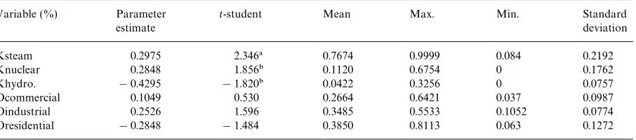
For the series of ine$ciency scores to take into account as the dependent variable, we have used that generated by the DEAc model.16 The DEA-based e$ciency scores are truncated from below at one. OLS regression would produce biased and inconsistent parameter estimates, so we use a truncated regression model (Tobit model). The estimated parameters are given in Table 6.
Given the statistical signi"cance of the three parameters used as proxies, it seems that the productive structure a!ects the e$ciency scores attained by the di!erent electric utilities. The market demand structure, on the other hand, seems not to have any in#uence.
Table 6
Tobit model estimated parameters
Variable (%) Parameter
estimate
t-student Mean Max. Min. Standard
deviation
Ksteam 0.2975 2.346! 0.7674 0.9999 0.084 0.2192
Knuclear 0.2848 1.856" 0.1120 0.6754 0 0.1762
Khydro. !0.4295 !1.820" 0.0422 0.3256 0 0.0757
Ocommercial 0.1049 0.530 0.2664 0.6421 0.037 0.0987
Oindustrial 0.2526 1.596 0.3485 0.5533 0.1052 0.0774
Oresidential !0.2848 !1.484 0.3850 0.8113 0.063 0.1272
!Signi"cant coe$cients at the 5% level (2-tailed).
"Signi"cant coe$cients at the 10% level (2-tailed).
Nuclear and even more so steam technologies seem to be exhausting their particular economies of scale.
The main problem of&two-stage'models, such as that used in this paper, is to know which regressors must be included in the estimation of e$ciency levels and which in their explanation. In the light of our results, besides their not being highly corre-lated with the variables utilised in the frontier estimation procedure, a necessary although not suf-"cient condition for regressors to be considered as proxies for ine$ciency sources is that they must be able to introduce heterogeneity in the analysis. Thus, a necessary extension to the empirical analy-sis that we have so far presented would be the introduction of additional information through variables properly representative of the industrial organisation, such as market structure, regulatory environment, ownership or internal organisation of the"rm.
4. Conclusions
The joint use of parametric and non-parametric techniques devoted to the measurement of e$cien-cy in the industrial sector is a novel issue in the recent empirical literature. However, this is not always feasible. Our paper has focused on the def-initions of a framework for the joint use of these techniques.
The main disadvantage of non-parametric approaches is their deterministic nature. DEA
tech-niques, for instance, make no accommodation for noise. Parametric techniques, as we have seen, require speci"cation of a particular technology for the frontier function as well as the de"nition of a speci"c statistical distribution for the ine$ciency term. The functional form requirement causes both speci"cation and estimation problems. Hence, the parametric}deterministic approaches for the measurement of productive e$ciency does not seem to be suitable for this kind of analysis. As our results suggest, they su!er from the disadvantages of both methods.
With respect to parametric}stochastic approa-ches, insofar as the disturbances about the frontier estimator tend to be symmetrically distributed, the frontier approach can be interpreted as a neutral transformation of the &average' technology. Then only Timmer's&Holy Grail'[35] i.e. the necessity of placing the frontier in order to give numerical values to e$ciency performances of each analysed unit, would justify a frontier approach instead of the traditional OLS-average approach. However, the presence of skewness in the disturbances is another reason why frontier functions might be taken into account: the underlying technology as-sumed under the average and the frontier speci"ca-tion can describe structural dissimilarities between the two techniques, such as di!erent returns to scale or elasticities of substitution.
relevant issues such as non-discretionary variables [36], categorical variables [37], or constrained multipliers [38]. Moreover, a recent paper [39] extends the use of DEA to a dynamic framework by incorporating changes in productivity due to tech-nological progress or regress. These aspects may correct some of the speci"cation problems asso-ciated with parametric methods.
The versatility of DEA techniques also provides a simple way of analysing the scale e$ciency. In our study, no relationship between the size of"rms and their ine$ciencies seems to exist. On the basis of the aforementioned robustness it is also possible to analyse the sources of productive ine$ciency by using two-stage models. These models will only be meaningful if the variables used as regressors intro-duce heterogeneity into the analysis.
We have here described some methodological considerations based on the data set used for this study. Much work remains to be done. For instance, additional information on prices and a larger sample of observations might improve the measurement of economic e$ciency in an indus-trial sector by taking into account technical and allocative e$ciencies as well as cost and revenue e$ciencies. As the literature shows, serious prob-lems arise when applying duality theory to para-metric frontier models. However, data envelopment analysis provides a suitable way of treating the
measurement of economic e$ciency. This
approach has been used in a number of empirical applications related to nonpro"t, regulated and private sectors. In conclusion, the present results provide encouragement for the continued develop-ment of the collaboration between parametric and non-parametric methods.
Acknowledgements
The authors are most grateful to two anonymous referees for their valuable comments.
References
[1] G. Debreu, The coe$cient of resource utilization, Econo-metrica 19 (1951) 273}292.
[2] T.C. Koopmans, An analysis of production as e$cient combination of activities, in: T.C. Koopmans (Ed.), Activ-ity Analysis of Production and Allocation, Cowles Com-mission for Research in Economics, New York, 1951. [3] M.J. Farrell, The measurement of productive e$ciency,
Journal of the Royal Statistical Society (A, general) 120 (1957) 253}281.
[4] A.N. Berger, Distribution-free estimates of e$ciency in the U.S. banking industry and tests of the standard distribu-tional assumptions, Journal of Productivity Analysis 4 (1993) 261}292.
[5] L.M. Seiford, R.M. Thrall, Recent development in DEA: the mathematical programming approach to frontier anal-ysis, Journal of Econometrics 46 (1990) 7}38.
[6] J.T. Sengupta, Data envelopment analysis for e$ciency measurement in the stochastic case, Computers and Operations Research 14 (1987) 117}169.
[7] J.T. Sengupta, Estimating e$ciency by cost frontiers: A comparison of parametric and nonparametric methods, Applied Economics Letters 2 (1995) 86}90.
[8] B.-J. Lee, Separability test for the electricity supply indus-try, Journal of Applied Econometrics 10 (1995) 49}60. [9] M. Nerlove, Returns to Scale in Electricity Supply,
Stan-ford University Press, StanStan-ford, CA, 1963.
[10] L.R. Christensen, W.H. Greene, Economies of scale in U.S. electric power generation, Journal of Political Economy 84 (4) (1976) 655}676.
[11] W. Greene, A gamma-distributed stochastic frontier model, Journal of Econometrics 46 (1990) 141}163. [12] G.D. Ferrier, C.A.K. Lovell, Measuring cost e$ciency in
banking: econometric and linear programming evidence, Journal of Econometrics 46 (1990) 229}245.
[13] S.C. Kumbhakar, The measurement and decomposition of cost-ine$ciency: The translog cost system, Oxford Eco-nomic Papers 43 (1991) 667}683.
[14] W. Greene, On the estimation of a#exible frontier produc-tion model, Journal of Econometrics 13 (1) (1980) 101}115. [15] M.I. Nadiri, M.A. Schankerman, The Structure of Produc-tion, Technological Change, and the Rate of Growth of Total Factor Productivity in the US Bell System, Academic Press, New York, 1981.
[16] S.C. Kumbhakar, A. Heshmati, L. Hjalmarsson, Temporal patterns of technical e$ciency: Results from competing models, International Journal of Industrial Organization 15 (5) (1997) 597}616.
[17] A. Gabrielsen, On estimating e$cient production func-tions, Working Paper no A-35, Chr. Michelsen Institute, Department of Humanities and Social Sciences, Bergen, Norway, 1975.
[18] J. Richmond, Estimating the e$ciency of production, International Economic Review 15 (1974) 515}521. [19] D.J. Aigner, C.A.K. Lovell, P.J. Schmidt, Formulation
and estimation of stochastic frontier production function models, Journal of Econometrics 6 (1977) 21}37. [20] W. Meeusen, J. van den Broeck, E$ciency estimation from
[21] G. Battese, G. Corra, Estimation of a production frontier model with application to the pastoral zone of Eastern Australia, Australian Journal of Agricultural Economics 21 (3) (1977) 167}179.
[22] J. Jondrow, C.A.K. Lovell, I.S. Materov, P. Schmidt, On the estimation of technical ine$ciency in the stochastic frontier production function model, Journal of Econo-metrics 23 (1982) 269}274.
[23] W.M. Greene, The econometric approach to e$ciency analysis, in: H.O. Fried, C.A.K. Lovell, S.S. Schmidt (Eds.), The Measurement of Productive E$ciency: Techniques and Applications, Oxford University Press, Oxford, 1993, pp. 68}119.
[24] A. Charnes, W.W. Cooper, E. Rhodes, Measuring the e$ciency of decision-making units, European Journal of Operational Research 2 (1978) 429}444.
[25] A.I. Ali, L.M. Seiford, The mathematical programming approach to e$ciency analysis, in: H.O. Fried, C.A.K. Lovell, S.S. Schmidt (Eds.), The Measurement of Produc-tive E$ciency: Techniques and Application, Oxford Uni-versity Press, Oxford, 1993, pp. 3}67.
[26] T. Coelli, D.S. Rao, G. Battese, An Introduction to E$ciency and Productivity Analysis, Kluwer, London, 1998.
[27] P. Schmidt, C.A.K. Lovell, Estimating technical and allocative ine$ciency relative to stochastic production and cost frontiers, Journal of Econometrics 9 (1979) 343}366.
[28] P. Schmidt, C.A.K. Lovell, Estimating stochastic produc-tion and cost frontiers when technical and allocative
inef-"ciency are correlated, Journal of Econometrics 13 (1980) 83}100.
[29] R. Fare, S. Grosskopf, J. Logan, The relative performance of publicily-owned and privately-owned electric utilities, Journal of Public Economics 26 (1985) 89}106.
[30] L. Hjalmarsson, A. Veiderpass, E$ciency and ownership in Swedish electricity retail distribution, The Journal of Productivity Analysis 3 (1992) 7}23.
[31] M.G. Pollit, Productive e$ciency in electricity transmis-sion and distribution systems, Oxford Applied Economics Discussion Paper Series, Vol. 161, 1994.
[32] S.C. Ray, K. Mukherjee, Comparing parametric and non-parametric measures of e$ciency: A reexamination of the Christensen}Greene data, Journal of Quantitative Econ-omics 11 (1) (1995) 155}168.
[33] J.D. Cummins, H. Zi, Comparisons of frontier e$ciency methods: An applications to the US life insurance indus-try, Journal of Productivity Analysis 10 (2) (1998) 131}152.
[34] C.A.K. Lovell, Production frontiers and productive e$ -ciency, in: O. Harold Fried, C.A.K. Lovell, S.S. Schmidt (Eds.), The Measurement of Productive E$ciency: Tech-niques and Application, Oxford University Press, Oxford, 1993, pp. 3}67.
[35] C.P. Timmer, Using a probabilistic frontier function to measure technical e$ciency, Journal of Political Economy 79 (1971) 579}597.
[36] R.D. Banker, R. Morey, E$ciency analysis for exogenous-ly"xed inputs and outputs, Operations Research 34 (4) (1986) 513}521.
[37] R.D. Banker, R. Morey, The use of categorical variables in data envelopment analysis, Management Science 32 (12) (1986) 1613}1627.
[38] A. Charnes, W.W. Cooper, Q.L. Wei, Z.M. Huang, Cone ratio data envelopment analysis and multi-objective pro-gramming, International Journal of Systems Science 20 (7) (1989) 1099}1118.