ON THE ESTIMATION OF RIGID-BODY TRANSFORMATION FOR TLS REGISTRATION
Marco Scaioni
Tongji University – College of Surveying and Geo-Informatics
Centre for Spatial Information Science and Sustainable Development Applications 1239 Siping Road, 200092 Shanghai, P.R. China
e-mail: marco@tongji.edu.cn
Commission V, WG V/3
KEY WORDS: Geo-referencing, Least Squares, Monte Carlo method, Reliability Analysis, Terrestrial Laser Scanning
ABSTRACT:
The paper presents some considerations on the estimation of rigid-body transformation which is the basis for registration and geo-referencing in terrestrial laser scanning. Two main issues are afforded, which in the opinion of the author have been poorly investigated up until now. The first one concerns the analysis of the stochastic model of Least Squares estimation of the transformation. In standard practice, the control points used for parameter estimation are considered as equally precise. Here two different approaches for weighting observations in laser scan and ground control points are proposed and evaluated through a set of Monte Carlo simulations. The second aspect refers to the reliability analysis. In particular the estimation of a joint-adjustment including both geo-referencing parameters and geodetic network observations for the determination of ground control points is discussed and evaluated.
1. INTRODUCTION
1.1 Terrestrial Laser Scanning today
Terrestrial laser scanning (TLS) is coming out from its pioneer epoch and nowadays is applied to many practical fields. In many of them it plays a paramount role today. On the other hand, in the first decade since its appearance, many tests and experimentations have been carried out in order to assess instruments and methods, to refine processes, and to explore new applications for engineering surveying, deformation measurements, topographic works, geology, architecture, archaeology and cultural heritage documentation, 3D visualization, and Virtual Reality.
On the other hand, some open problems still exist. These could be summarized in the following items:
• standardization of instrument metrological features and methods for their evaluation;
• definition of standard procedures for geo-referencing, scan planning, automatic co-registration of multiple scans; and
• definition of application domains where the use of TLS is really worth, and where other techniques can be more fruitful (e.g. photogrammetry).
In the meantime, manufacturers have pushed up the diffusion of laser scanners, and purchasers have become familiar to the use of this technique for production work and research activity. Very often the way they used TLS are limited to procedures proposed in vendor reference guidelines, without any critical analysis. This fact should be considered with great care, considering the recent increase of the interest for high precision applications, such as modelling of industrial sites (see Rabbani, 2006) and deformation measurement (see Vosselman and Maas, 2010). Here any step of the acquisition and processing of TLS data must be operated with the highest carefulness.
The basic geometric model implemented in laser scanning processing is the rigid-body transformation. A lot of work has been carried out so far on the estimation of the 6 parameters that are incorporated into this model (3 shifts and 3 rotations in space). Several aspects have been investigated, such as: evaluation of approximate values through linear or closed-form solutions, robust estimation, automatic labeling of corresponding points, integration of laser scans and images for mutual registration purpose.
Such rigid-body transformation has been integrated by additional parameters to compensate for calibration errors (see Lichti, 2010). These solutions can be exploited to refine laser scanning measurements in applications where high accuracy is needed. Recently, different papers referred to a deeper analysis on the contribution of different error sources to the whole error budget of TLS measurement (Gordon and Lichti, 2005; Scaioni, 2005). Indeed, inclination of incident laser beam, diverse material reflections and other effects can result in discrepancies from the standard geometric model.
The paper mainly affords two main issues, which in the opinion of the author have been poorly investigated up until now. The first one concerns the Least Squares estimation of the rigid-body transformation. In the standard practice, points used for parameter estimation are considered as equally precise. On the other hand, if a scan is registered to ground or to another scan taken as reference, only points in one scan are usually considered as stochastic observations. To consider both problems, a formulation of the Least Squares rigid-body transformation estimation including a pointwise weighting in both reference systems (scan to ground or scan 1 to scan 2) is applied in Section 2. Some considerations based on different point configurations are reported to show when this approach is worth to be used.
The second aspect refers to the reliability analysis, i.e. the chance to detect gross errors in observations. Which are the factors that can improve this important property? In many close-range applications, ground control points (GCP) are measured International Archives of the Photogrammetry, Remote Sensing and Spatial Information Sciences, Volume XXXIX-B5, 2012
within a local geodetic network. Errors in geodetic and laser scanning measurements can be at the same order. Consequently, a joint-adjustment of both sets of observations would be an option to increase the inner reliability. Some theoretical considerations about this solution and a simulated case are reference system (RS). In the following, the instrumental RS of the scan i-th is termed Intrinsic RS (IRSi). If an external geodetic datum is established, this is referred to as Ground RS (GRS); in this case, the registration of one or more scans into the GRS is addressed to as the geo-referencing problem. The geometric model usually adopted for registration or geo-referencing is a 3D rigid-body transformation, possibly integrated by a set of parameters for laser scanner calibration:
ij
AP : vector including additional parameters for calibration in IRSi;
∆xjAP : vector including additional parameter for calibration of points in IRSj (∆xjAP=0 if IRSj≡GRS).
The computation of unknown parameters is carried out on the basis of common features (usually points are used) in both RSs. On the other hand, in practical applications, the geometric model (1) is rarely integrated with further additional parameters to correct errors due to non-modelled systematic effects (∆xAP). However, when this happens (see e.g. Lichti, 2008), the calibration is performed at a preliminary stage by measuring a test-field made up of tens of GCPs or other kinds of features (e.g. planes), and the results applied to correct the x2i vector in (1).
The estimation of the unknown parameters of geometric model (1) is usually carried out by Ordinary Least Squares (OLS), after linearization (Wolf and Ghilani, 1997). This requires the computation of approximations for all parameters, which can be derived by a twofold strategy. The first one relies on the use of an algorithm which can perform the solution of Eq. (1) without any initial values. Three main approaches are adopted based on Procrustes analysis (Beinat et al., 2000), Hamilton’s Quaternions (Horn, 1987), Orthonormal transformations (Horn et al., 1998). At the first stage, often the automatic search for correspondent features in both IRSi and IRSj is applied (Bornaz et al., 2003). Furthermore, a high breakdown-point estimator
referencing technique (Scaioni, 2005), approximations of parameters are already known.
2.1.1 Functional model for Ordinary Least Squares
The functional model for OLS defines the linear (or linearized) relation between observations and parameters to estimate. According to the formulation based on observation equations, points measured in scan i-th (xi) are organized in the vector y0. These are function of the points measured in scan j-th (xj) as well as the corrections to registration parameters (dβ1), to be estimated through eq. (1) after linearization. To consider also points in scan j-th as stochastic variables, they are introduced as further unknowns (dβ2). Consequently two groups of equations are setup. The first comprehends the observation equations:
c should be included in the functional model:
d dβ
w=D2 2+ . (3)
To account for the uncertainty of observations, two weight matrices are adopted (Wi, Wj) for points observed in scans i-th and j-th, respectively. Three relevant options for the weight matrices are thoroughly analysed in Paragraph 2.1.2.
2.1.2 Stochastic model
In the most applications, only points in the scan i-th are considered as stochastic variables (cases ‘a’ and ‘b’).
In the case ‘a’, all measured points have the same precision. The standard model for error distribution is the hysotropic Gaussian distribution, assumption that only approximately corresponds to reality. Indeed, the use of the same weights for all points is not correct. Indeed, measurement errors in laser observations (angles and ranges) are not hysotropic. Moreover, some error sources in laser measurements are not normally distributed (e.g. the effect of laser beamwidth and surface reflectivity – Lichti et al., 2005). Although the Central Theorem of Statistics supports the use of the Gaussian model, this is only an approximation. Indeed, the most error sources are neglected in the stochastic model because they are difficult to quantify. Some results have been published about the effects of surface orientation with respect to laser beam (Bae et al., 2009). However, this approach is difficult to follow in the practice. Here a simple solution for weighting points in a scan is used (case ‘b’), by adopting the ‘positional’ model proposed in Alba et al. (2010). The precision of each point k in the scan can be expressed through the International Archives of the Photogrammetry, Remote Sensing and Spatial Information Sciences, Volume XXXIX-B5, 2012
(θ). When an algorithm for automatic target measurement is adopted, a further contribute to the error budget can be added up by introducing related variances and covariances (indicated with sub-index ‘FM’). The matrix (4) in polar coordinates has to be propagated to obtain the one in Cartesian coordinates (C′k) needed for the estimation of parameters of Eq. (1). Then the covariance matrix (C) of all the observed points in the scan will result from the composition of all matrices C′k into a block-diagonal structure. Consequently the weight matrix will be W= C-1. On the other hand, other more involved error models can be used, like that proposed in Bae et al. (2009). In any case, when operating with real datasets, the effectiveness of the adopted method depends upon how well the error model fits real observations. On the other hand, simulated data allows to understand which contribute can be achieved from the use of weighted observations.
A third case (‘c’) takes into consideration also weighted observations in both scans i-th and j-th. Both weight matrices W1 and W2 can be defined as in case ‘b’. This formulation is adequate to describe the co-registration of two laser scans in the RS of one of them. If the RS of one scan is given by GCPs, these can be weighted by adopting the estimated precision obtained from the LS adjustment of the geodetic network.
2.2 Monte Carlo analysis of stochastic models
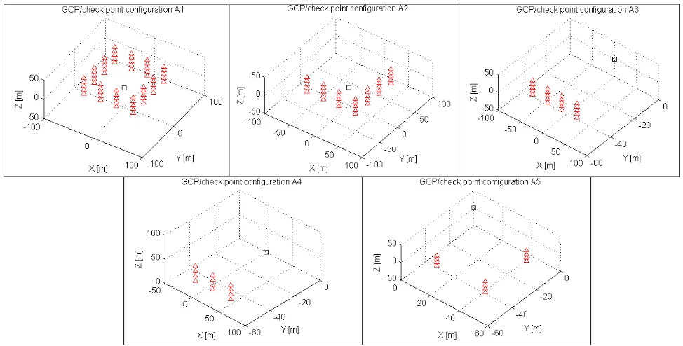
Five simulated datasets have been setup with various numbers of points and spatial distribution (Fig. 1). In each of them, a laser scan has been acquired from a central position with respect to a set of targets to be used as GCP for geo-referencing. Instrument precision is that typical of a medium range phase-shift modern scanner (σρ=±5 mm; σα=σθ=±0.05 mrad). The ‘positional’ error model (4) has been adopted to simulate measurement errors. The precision of target measurements or the presence of systematic errors has been neglected here. In the cases ‘a’ and ‘b’ the GCPs have been considered as error-free. In the case ‘c’ they have been weighted by using the estimated theoretical accuracies from geodetic network adjustment.
A Monte Carlo simulation (Robert and Casella, 2004) has been applied to all datasets to compare diverse weighting strategies. The evaluation of results is possible because the true value of points is known here. This makes possible to analyse either residuals on error-free independent check points and parameters. This is obviously a great advantage to verify the adequacy of different stochastic models under investigation. On the other hand, simulations do not allow one to assess how the assumed models fit with real data.
Monte Carlo simulation is based on the repetition of a high number of trials where input data are randomly extracted based on a probabilistic distribution. Here the simulated observations consist on a set of corresponding points which have been measured in both IRS and GRS. A set of preliminary experiments have been carried out to setup the minimum number of trials (ntr) giving enough stability to the results. Once a value ntr=10000 is decided, 10 sets of experiments with the same number of trials has been repeated to assess the repeatability of results. This assumption has been verified, considering that all outcomes differ less than the assumed data uncertainty.
2.3 Results of simulations
Configurations from A1 to A4 have been designed to progressively reduce stability. This result has been obtained by either decreasing the total number of points, and by weakening their spatial distribution. In configuration A5 a small set of points (#12) like in A4 has been setup, but with a stronger geometry.
The quality of geo-referencing has been evaluated by computing residuals on error-free check points. Two groups of check points have been analysed. The first collects all points of dataset A1 and allows evaluating the global quality of the estimated geo-referencing. The second group comprehends only those points contained in the region internal to the GCPs. Indeed, best practices always suggest selecting GCPs around the area to survey.
Figure 1. – GCP configurations adopted in Monte Carlo simulations to assess different stochastic models. International Archives of the Photogrammetry, Remote Sensing and Spatial Information Sciences, Volume XXXIX-B5, 2012
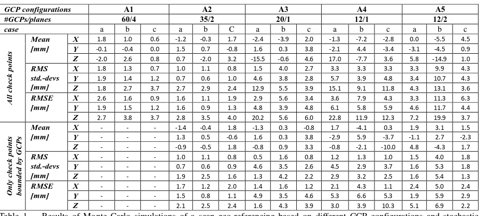
GCP configurations A1 A2 A3 A4 A5 models (‘a’: uniform weighting of laser scanner observations only; ‘b’: weighting laser scanner observations based on the ‘positional’ model; ‘c’: using also weights for GCPs). Results refer to the use of two different groups of check points.
In general, computed residuals on check points have resulted smaller in the second subset than in the first group, as expected. Although there is not full evidence that a stochastic model is absolutely better than another, two conclusions can be drawn. In the most stable configurations (A1-A2) all stochastic models worked well. As far as the configuration becomes weaker, the case ‘c’ showed slightly better results than ‘b.’
2.4 Criterion matrix
The simulations’ outcomes suggest checking the spatial distribution of points to detect possible weak configurations. Such kind of criteria is also important in estimation techniques (e.g. RANSAC or Least Median of Squares) based on random one to establish if the current point configuration is better than expected, according to H. Here the approach proposed in motivated by the observation that if H is setup based on an ideal configuration, the number of points in here might strongly affect the results with respect to their spatial distribution. Alternatively, Förstner (2001) suggests to compute H based on
some theoretical considerations on variances and correlations between parameters.
In Table 2 the results of test (6) for the 5 GCP configurations in Figure 1 are shown. In addition, some subsets of points have been derived from the largest dataset A1. While a homogenous spatial distribution of points has been kept, their number has configurations with a criterion matrix from case A1.
3. RELIABILITY ANALYSIS
3.1 Basics concepts
Reliability refers to the chance to detect gross errors in the target coordinates measured in the laser scan and adopted for geo-referencing purpose. The same concept could be extended to include also errors in GCP coordinates, but this case is not considered here.
The problem is to evaluate how big can be the error on estimated geo-referencing parameters of a scan, according to the largest theoretical error in observations that cannot be theoretically detected by data snooping (Baarda, 1968). The inner reliability relates the expectation E(|vi|)≠0 (also called non-centrality parameter δ0) of the normalised correction corresponding to a gross error ∆li which is locatable with a given probability 1-β:
( ) ( )
li estimated parameters x from LS adjustment. The corresponding outer reliability is then given by the expression:( )
∆x =(
T)
−1 T E( )
∆lE A WA A W . (8)
Vector E(|∆l|)is zero except on the element corresponding to the observation affected by gross error ∆li.
3.2 Analysis of simulated configurations
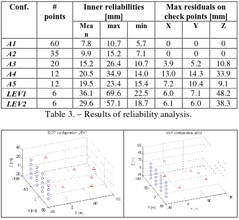
A reliability analysis of the configurations adopted in Section 2 has been carried out. A non-centrality parameter δ0= E(|vi|)=4.0, a significance α=0.01 and a power β=0.93 have been setup. The corresponding rejection threshold for data snooping is k=2.56. In Table 3 some results on the inner reliabilities computed for points in configurations A1, A2, A3, A4, and A5 are reported. As can be seen, in the less stable configurations (A4-A3-A5) the largest inner reliabilities can reach some centimetres.
Assuming that in the dataset is present only one gross error which is equal to the largest inner reliability value, this will lead to a bias in the estimated geo-referencing parameters. This can be computed based on Eq. (8). To better understand the effect of this error on the final point coordinates, each biased set of parameters has been used to compute the discrepancies on the check point coordinates. As can be seen in Table 3, the effect on check points of the largest undetectable error in observations is quite relevant for weak configurations. On the other hand, no significant effects can be noticed in the strongest ones (A1-A2). This outcome highlights the need of major care on reliability analysis during geo-referencing, especially in high-precision applications.
3.3 Leverage points
Leverage points in regression estimation are meant to be points which have a strong influence on the estimated result. This is due to their geometric position, especially in the case of non-homogenous or unbalanced data. Such points are characterized by a low local redundancy, and the corresponding residuals can mask larger errors. The corresponding inner reliability will be larger, according to Eq. (7).
Table 3 reports the inner reliabilities computed for all datasets in Section 2. It is evident how no leverage points appear in configurations A1 and A2, due to the large number of data and their good spatial distribution which result in quite even inner reliabilities. The result is different in smaller and asymmetric configurations like A3, A4 and A5. Here there are some points with higher inner reliabilities than average values. Two new small datasets (see Fig. 2) have been setup for the purpose of investigating the existence of leverage points (LEV1 and LEV2). The lower rows of Table 3 show how dramatic is the problem here. If in general the average inner reliabilities are large due to the poor data redundancy, some observations lead to undetectable errors up to several centimetres, as can be seen in the rightmost three columns of Table 3. Here the maximum residuals on check points depending on the error on the
observation with the largest inner reliability have been computed based on Eq. (8). In reality, the situation can be also worse because observations in TLS are strongly correlated among them. Indeed, here the coordinates of targets in a scan
Table 3. – Results of reliability analysis.
Figure 2. – GCP configurations with leverage points; red triangles are GCP, blue circle check points that are outside the bounding box of GCP to simulate a typical scenario in deformation measurements.
3.4 Joint-adjustment of laser scan and geodetic data
A further chance to increase the local redundancy of laser scan observations is to combine the adjustment for computing geo-referencing parameters to the one of the geodetic network for the determination of GCP coordinates. The procedure is similar to joint-adjustment that was experienced in aerial photogrammetry.
The design matrix A is made up of different sub-matrices. Observation equations coming from linearization of Eq. (1) contribute to both sub-matrix Ap (size 3n×6, where n is the number of points), containing the coefficients of geo-referencing parameters, and to AGCP (size 3n×3n), with the coefficients of GCPs. Three different kinds of theodolite measurements can be adopted in a geodetic network for working out GCP coordinates: azimuth and zenith angles, slope distances. The geodetic datum can be setup thanks to the knowledge of the stations’ coordinates, or by arbitrarily fix them to establish a minimum constraint. This second group of observation equations gives rise to sub-matrix Ag (size h×3n, where h is the number of geodetic observations). The full design matrix A and the weight matrix W of joint-adjustment is then and geodetic observations, respectfully. The redundancy matrix can be computed as follows:
(
A WA)
A W AI
R= − T −1 T . (10)
Reckoning how much is the contribution of geodetic observations to local redundancies is not directly possible from Eq. (10). Conversely, an approach based on simulating a typical geodetic network for the determination of 10 GCPs has been followed. Coordinates of GCPs are measured thanks to geodetic measurements from 3 stations. These are considered known with superior accuracy. They also establish the GRS. Coordinates of GCPs are also observed in the laser scan. Table 4 shows the number of equations and unknowns in both cases of joint-adjustment and independent adjustment of geodetic network and geo-referencing parameter estimation.
Geodetic observations can be weighted with easy on the basis of instrumental precisions. On the other hand, TLS measurements of targets are more difficult to predict. The results can be divided in three groups, according to weights:
1. homogeneous weights: the ‘positional’ model has been adopted to find reasonable values for weights in TLS. In this case, the joint-adjustment leads to an average decrease of the local redundancies of TLS observations (-17%), while those of geodetic observations rise up of +6.7%;
2. increasing weights of TLS data: if targets in the laser scan are measured with higher precision (5 times the previous case), they results in a significant average improvement of local redundancies of the geodetic observations (+33.2%). Conversely, the ones of TLS measurements dramatically drop down (-82.9%); and
3. decreasing weights of TLS data: if targets in the laser scan have been measured with lower precision (5 times worse than in case 1), the average change of local redundancies is very small (+0.3% for TLS and -0.8% for geodetic observations, respectively).
The results tell that with better laser scan measurements it is possible to control geodetic observations, but not the contrary. However, all the intermediate cases strictly depend upon a proper evaluation of weights. Thus they do not seem useful in the practice.
Equations Unknowns Global
redundancy
Geod. TLS Geod. TLS
Geodetic 90 - 30 - 60
TLS - 30 - 6 24
Joint-adj. 90 30 30 6 84
Table 4. - Features of independent and joint-adjustment for estimating geo-referencing parameters and GCP coordinates.
4. CONCLUSIONS AND FUTURE DEVELOPMENTS
In recent years terrestrial laser scanning (TLS) techniques have achieved a great success in many domains. For the most this is due to the straightforward acquisition of 3D data and to the simplification of the registration procedures with respect to photogrammetry. In many practical applications, today TLS allows users to accomplish projects that in the past required a much higher effort. On the other hand, a different approach should be followed in the case of high-precision applications, likewise deformation monitoring.
Although much work has been carried out on modelling systematic errors, automation of laser scan registration, and
point cloud segmentation, less attention has been put on design of data acquisition and quality assessment. In close-range photogrammetry, paramount work on these topics was carried out in the ‘80s and ‘90s. This paper is a short attempt to draw the attention of TLS researchers and practitioners on some of these concepts.
The development of stochastic models that can be suitable to deal with real data is an important issue, especially when dealing with weak configurations in geo-referencing. The reliability analysis has been demonstrated to play a fundamental role in high-precision applications. Here the case of single scan registration to ground has been considered. The same analysis could be extended to the case of several scans to be registered in a common frame.
Acknowledgements
Aknowledgements go Kwang Hua Foundation, Tongji University, (Shanghai, P.R. China).
REFERENCES
Baarda, W., 1968. A Testing Procedure for Use in Geodetic Networks. Netherlands Geodetic Comm. New Series 4, Delft.
Baarda, W., 1973. S-Transformations and Criterion Matrices. Netherlands Geodetic Comm. New Series 4 Delft.
Bae, K.-H., Belton, D. and D.D. Lichti, 2009. A Closed-Form Expression of the Positional Uncertainty for 3D Point Clouds. IEEE Trans. Pattern Anal. Mach. Intell. 31(4): 577-590.
Beinat, A., Crosilla, F., and D. Visintini, 2000. Examples of georeferenced data transformations in GIS and digital photogrammetry by Procrustes analysis techniques. Int. Archives of Photogrammetry and Remote Sensing (IAPRS), Vol. 32, Part 6W8/2, Lubljana, Slovenia, 6 pp.
Bornaz, L. Lingua, A. and F. Rinaudo, 2003. Multiple scan registration in LIDAR close range applications. IAPRS, Vol. 34, Part 5/W12-V, Ancona, Italy: 72-77.
Förstner, W., 2001. Generic Estimation Procedures for Orientation with Minimum and Redundant Information. In: Grün, A. and T.S. Huang (eds.), Calibration and Orientation of Cameras in Computer Vision, Springer-Verlag, Berlin Heidelberg (Germany), pp. 63-94.
Gordon, S.J. and D.D. Lichti, 2005. Terrestrial laser scanners with a narrow field of view: The effect on 3D resection solutions. Survey Review 37(292): 448-468.
Horn, B.K.P., 1987. Closed-from solution of absolute orientation using unit quaternions. J. Opt. Soc. Amer. A 4(4): 629-642.
Horn, B.K.P., Hilden, H.M. and S. Negahdaripour, 1998. Closed-form solution of absolute orientation using orthonormal matrices. J. Opt. Soc. Amer. A 5(7): 1127-1135.
Lichti, D.D., Gordon, S.J. and T. Tipdencho, 2005. Error Models and Propagation in Directly Georeferenced Terrestrial Laser Scanner Networks. Journal of Surveying Engineering 131(4): 135-142.
Lichti, D.D., 2010. A review of geometric models and self-calibration methods for terrestrial laser scanners. Boletim de Ciencias Geodesicas
16(1): 3-19.
Rabbani, T., van den Heuvel, F.A., and G. Vosselman, 2006. Segmentation of point clouds using smoothness constraints. Int. Archives of the Photogrammetry, Remote Sensing and Spatial Information Sciences (IAPRS&SIS), Vol. 36, Part 5/A, Dresden, Germany: 248-253.
Robert, C.P. and G. Casella, 2004. Monte Carlo Statistical Methods (2nd edition). Springer-Verlag, New York.
Rousseuw, P.J. and Leroy, A.M. ,1987. Robust Regression and Outlier Detection. John Wiley, New York, 329 pages.
Scaioni M., 2005. Direct Georeferencing of TLS in Surveying of Complex Sites. IAPRS&SIS, Vol. 36, Part 5/W17, 8 pp (on CDROM). Vosselman, G., and H.-G. Maas, 2010. Airborne and Terrestrial Laser Scanning. Whittles Publishing, Caithness, Scotland (UK).