MASS BALANCE CHANGES AND ICE DYNAMICS OF GREENLAND AND ANTARCTIC
ICE SHEETS FROM LASER ALTIMETRY
G.S. Babonisa, B. Csathoa,∗, T. Schenka
a
Dept. of Geology, University at Buffalo, 126 Cooke Hall, Buffalo, NY 14260, U.S.A. - (afschenk, bcsatho)@buffalo.edu
Commission VIII, WG VIII/6
KEY WORDS:Laser Atimetry, Surface Elevation Changes, Greenland, Antarctica, Ice Sheet Mass Balance, Sea-Level Rise.
ABSTRACT:
During the past few decades the Greenland and Antarctic ice sheets have lost ice at accelerating rates, caused by increasing surface temperature. The melting of the two big ice sheets has a big impact on global sea level rise. If the ice sheets would melt down entirely, the sea level would rise more than 60 m. Even a much smaller rise would cause dramatic damage along coastal regions. In this paper we report about a major upgrade of surface elevation changes derived from laser altimetry data, acquired by NASA’s Ice, Cloud and land Elevation Satellite mission (ICESat) and airborne laser campaigns, such as Airborne Topographic Mapper (ATM) and Land, Vegetation and Ice Sensor (LVIS). For detecting changes in ice sheet elevations we have developed the Surface Elevation Reconstruction And Change detection (SERAC) method. It computes elevation changes of small surface patches by keeping the surface shape constant and considering the absolute values as surface elevations. We report about important upgrades of earlier results, for example the inclusion of local ice caps and the temporal extension from 1993 to 2014 for the Greenland Ice Sheet and for a comprehensive reconstruction of ice thickness and mass changes for the Antarctic Ice Sheets.
1. INTRODUCTION
The Greenland and Antarctic ice sheets contain more than 99 % of the freshwater ice on Earth, and thus, they are important contributors to global sea level rise. If they were melted com-pletely, sea level would rise by 66 meters. Rapid warming has caused a dramatic decrease of ice in the Artic region during last few decades. Sea ice extent rapidly declined; glaciers sped up, thinned and retreated, and permafrost warmed up and thinned. Arctic warming is further amplified as surface temperature in-creases due to the melt of the protective snow and ice cover. The Greenland Ice Sheet (GrIS) has lost an average 250 Gt/yr ice an-nually, equivalent to 0.7 mm/yr sea-level rise, since 2003. There remains much uncertainty in estimating the current mass loss of the Antarctic Ice Sheet (AIS). While vast regions of the West Antarctic Ice Sheet exhibit increasing ice loss in its marine-based regions, increasing snowfall or long-term dynamic thickening of the East Antarctic Ice Sheet might balance this ice loss.
Here we present a comprehensive update of Greenland and Antarc-tic Ice Sheet surface elevation changes obtained from the laser al-timetry record using our Surface Elevation And Change detection (SERAC) software suite (Schenk and Csatho, 2012). We have de-veloped SERAC to derive information from laser altimetry data, particularly time series of elevation changes and their partitioning into changes caused by surface processes and ice dynamics. This partition allows direct investigation of ice dynamic processes that is much needed for improving the predictive power of ice sheet models.
This latest reconstruction of GrIS elevation changes consists of 130,000 ice-sheet elevation change time series, spanning 1993-2014, derived from satellite laser altimetry data acquired by NASAs Ice, Cloud and land Elevation Satellite mission, airborne laser observations obtained by Airborne Topographic Mapper (ATM) and the Land, Vegetation and Ice Sensor (LVIS). This work pro-vides a major upgrade of the results presented in our latest study
∗Corresponding author
(Csatho et al., 2014), by extending the temporal coverage and by including local ice caps and glaciers. We also present the first synoptic reconstruction of ice sheet elevation changes of the AIS, derived from ICESat observations spanning the period of 2003-2009. For both ice sheets, elevation changes are partitioned into components due to vertical crustal deformations, firn-compaction and ice dynamics, and are converted into mass changes.
2. METHODOLOGY
We have developed the comprehensive Surface Elevation Recon-struction And Change detection (SERAC) method to determine surface changes by a simultaneous reconstruction of the surface topography (Schenk and Csatho, 2012). Although general in the design, SERAC was specifically developed for detecting changes in ice sheet elevation from ICESat crossover areas. It addresses the problem of computing a surface and surface elevation changes from discrete, irregularly distributed samples of the changing sur-face. In every sampling period, the distribution and density of the acquired laser points is different. The method is based on fit-ting an analytical function to the laser points of a surface patch, for example a crossover area, size1 km×1 km, or within re-peat tracks, for estimating the ice sheet surface topography. The assumption that a surface patch can be well approximated by ana-lytical functions, e.g. low order polynomials, is supported by var-ious roughness studies of ice sheets (Van Der Veen et al., 1998, Van Der Veen et al., 2009). Considering physical properties of solid surfaces and the rather small size of surface patches sug-gest that the surface is only subject to elevation changes but no significant deformations. That is, the shape of surface patches remains constant and only the vertical position changes. It is im-portant to realize that SERAC determines elevation changes as the difference between surfaces, unlike other methods that take the difference between identical points of two surfaces.
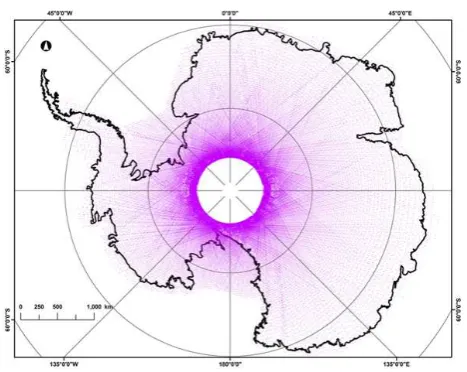
Figure 1. Location of times series locations in Antarctica gener-ated by SERAC at ICESat ground track crossovers.
Since there are many more laser points than unknowns, surface elevation and shape parameters are recovered by a least squares adjustment whose target function minimizes the square sum of residuals between the fitted surface and the data points. The large redundancy makes the surface recovery and elevation change de-tection very accurate and robust. Moreover, the confidence of the results is quantified by rigorous error propagation.
Moreover, while most other studies do not compute more than an average elevation change rate, SERAC reconstructions incorpo-rate elevation observations from all different time periods cover-ing a crossover area to generate a time series of elevation changes that is referred to the centroid of the crossover region. SERAC also provides error estimates for each reconstructed surface ele-vation within the time series. Thus, the SERAC method is able to capture important interannual variations that are not recognized by methods that assume a constant elevation change rate.
2.1 Antarctica
We reconstructed surface shape and elevation changes from the complete ICESat observational record at all ICESat crossover re-gions to generate approximately 110,000 elevation change histo-ries for the time period of 2003-2009 (Fig. 1). The crossovers are densest around 86o
S, where ground track spacing approaches 0 km in separation, and less dense in coastal regions where ground track spacing can be as wide as 30 km. While crossovers provide a less dense coverage of the ice sheet than repeat-track measure-ments, they allow for a robust reconstruction of surface elevation changes, whereas the correlation between cross-track slope and elevation changes between repeat observations limits the accu-racy of the along-track solutions.
The resulting elevation change histories are filtered in a multi-step process that identifies and removes erroneous change histo-ries based upon spatial boundahisto-ries as well as the elevation change data contained in each history. First, all crossover locations out-side of grounded ice, with boundaries defined by the MODIS Mo-saic of Antarctica (e.g. ice-shelves, and ice-sheets boundaries and grounding lines; freely distributed through the National Snow and Ice Data Center ((Haran, 2005), https://nsidc.org/data/moa/ )), are removed from further processing. To account for observations within the grounding line, but over exposed bedrock, a landcover mask, also derived from the MODIS Mosaic of Antarctica, was used to remove all elevation change histories within 500 m of exposed rock outcrops.
Remaining SERAC time series are examined for goodness of fit between the original laser points and the third order polynomial surface fitted by SERAC as well as for the distribution of eleva-tion observaeleva-tions contributing to the reconstruceleva-tion, as measured by the spatial fitting error and the condition number, respectively (Schenk and Csatho, 2012). Those time series exhibiting large elevation uncertainties are removed from further processing. In order to assert long enough temporal coverage to adequately ex-amine inter-annual changes over Antarctica, any of the remaining elevation change histories with less than three years of total cov-erage between the first and last observation were removed from further processing. Additionally, of those remaining histories, any that did not have at least five unique time epochs worth of coverage were also removed from further processing. To account for variations in elevation changes at the calving fronts of outlet glaciers due to ice retreat during the observational time period, any crossover regions whose centroid was within 10 m from the EGM 2008 geoid surface was excluded from further processing.
During the final filtering step, elevation change histories exhibit-ing localized non-linear dynamic thickness change trends are iden-tified, and removed from further processing. This was done for two reasons: 1.These events reflect very localized changes in ice sheet thickness, in contrast to regional surficial processes or dy-namic changes which are more important factors in determining regional ice behavior. 2. Short term, large amplitude changes are likely caused by hydrologic events such as the direct redistri-bution of subglacial water, through infilling and drainage, or by localized changes in subglacial basal shear stress, as in the case of sticky spots (Sergienko and Hulbe, 2011).
After performing the filtering steps described above and remov-ing the curves indicatremov-ing short-term rapid changes, the remain-ing 92,000 elevation change histories were corrected for verti-cal crustal motion using postglacial rebound rates from the w12a Antarctica GIA model (Whitehouse et al., 2012) and partitioned into thickness changes related to surface processes and ice dy-namics (Figure 2). Elevation changes due surface processes were taken from a semi-empirical firn densification model (FDM) of Antarctica ((Ligtenberg et al., 2011)), driven by the Regional At-mospheric Climate Model 2 (RACMO2, (van Meijgaard et al., 2008)). This model accounts for elevation changes due to sur-face mass balance anomalies and the processes of firn densifica-tion into ice over time. Dynamic ice thickness changes are com-puted as the difference between the total ice thickness change and the ice thickness change caused by surficial processes. It should be noted that other studies have reported the presence of additional instrument-related elevation bias between ICESat campaigns (Hofton et al., 2013, Siegfried et al., 2011, Zwally et al., 2015). However, as no current agreement exists regarding an inter-campaign bias correction (IBC) the data in this study have not be adjusted for it during processing.
The total and dynamic thickness changes were fit with a third order polynomial approximation in the time domain and thick-ness changes were sampled from these polynomial approxima-tions at the beginning and the end of each Antarctic balance years (March 1 and February 28/29), during the ICESat operational pe-riod (March 1, 2003-February 28, 2009) to calculate annual thick-ness change rates at each crossover location. In order to identify potential outliers from the polynomial approximation process, mean annual thickness change rates were calculated for each year and those crossover with at least one annual value outside three standard deviations from the annual mean was flagged and man-ually inspected.
It is important to note that the annual changes from 2003-2004 are more limited in spatial resolution than other balance years. The International Archives of the Photogrammetry, Remote Sensing and Spatial Information Sciences, Volume XLI-B8, 2016
Figure 2. Total, surficial process (SMB and firn-compaction) and ice dynamic related ice sheet thickness changes, examples from Antarctica. Left: Pine Island Glacier (630 meter), right: EAIS Plateau (3,331 meter).
This is due to two factors: (1) The ICESat mission began in February 2003 with data collection along sparsely distributed 8-day repeat ground-tracks to support sensor calibration; and (2) Data acquisition along densely distributed 183-day repeat ground tracks started on March 21 (L1B), but on March 29 2003, Laser 1 of the GLAS instrument failed prematurely, thereby reducing the amount of data collected in the beginning of the mission. Data ac-quisition commenced again on September 29 (L2A), when Laser 2 was turned on a 24-day period. Due to this limitation, annual results from 2003-2004 are not examined in this study.
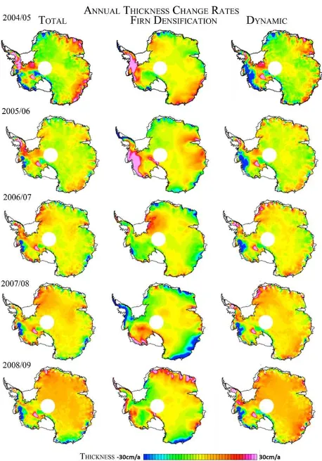
The annual change rates were gridded at 25 km postings for each balance year from 2004-2009 (Fig. 3), using Ordinary Kriging in Geosoft Oasis Montaj 8.2. The annual change rate grids were then resampled to 5 km postings, and filtered using a land-cover classification to remove regions of exposed bedrock and regions outside of the grounding line.
Figure 3. Annual total, surficial process (SMB and firn-compaction) and ice dynamic related thickness change rates, Antarctica.
2.2 Greenland
We used our SERAC system to determine ice sheet elevation changes with up to four repeat ICESat missions per year and with additional ATM and LVIS flights to obtain a comprehen-sive record for the ICESat period 2003-2009. SERAC is able to handle simultaneously different laser altimetry sensors, such as ICESat, and NASA’s airborne sensors ATM and LVIS. This feature enables the increase of the temporal domain of time se-ries and at the same time densifies their spatial positions. The spatial densification is particularly useful in coastal areas where the ICESat tracks are widely separated. Moreover, he magnitude of thickening and thinning patterns of the outlet glaciers require denser sampling than ICESat can provide. Equally important is the temporal extension to 1993-2014, going back in time to the first ATM observations (1993) and forward to current times by including the most recent laser altimetry observations provided by NASA’s Operation IceBridge mission.
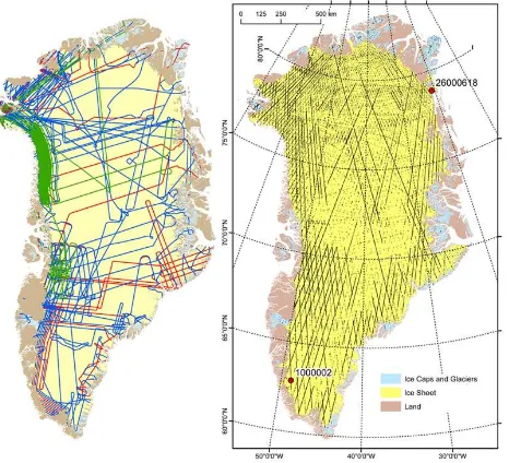
Figure 4. Left panel: ATM (2013, red lines; 2014, blue lines) and LVIS (2013, green lines) trajectories over the Greenland Ice Sheet (yellow) and local ice glaciers and peripheral ice caps (blue). Ice sheet, ice caps and glacier boundaries are from Rastner et al., 2012. Ice sheet is shown in yellow and local glaciers and ice caps are blue. Right panel: location of SERAC times series (black dots) generated from the combined 1993-2014 ICESat, ATM and LVIS data sets.
Figure 5. SERAC elevation time series illustrating the fusion of ICESat (blue dots) and ATM (red dots) altimetry data from the Jakobshavn drainage basin, West Greenland. The good agree-ment between the elevations derived from ICESat and ATM ob-servations confirms the excellent accuracy of the laser systems.
3. RESULTS
3.1 Antarctica
Fig. 3 shows the annual total, surface process related (FDM) and dynamic thickness change rates between 2004 March 1 and 2009 February 28 and the mean annual dynamic thinning rate is pre-sented in Fig. 6.
These results illustrate the complex nature of ice behavior across Antarctica. In the Pine Island Glacier region (Fig. 6: 1), where warming ocean temperatures quickly erode the ice lying below sea level, surface elevation exhibit widespread regional thinning of over 2 meters per year during the full time period of the study. Further along the coast from Pine Island Glacier, the Sulzberger Ice Shelf demonstrates steady dynamic thinning, in contrast to
Figure 6. Upper panel: mean annual dynamic thickness change rate (March 1 2004 - February 28 2009). Numbers mark re-gions with distinct thickness change patterns described in the text. Lower panel: error of mean annual dynamic thickness change rate map (left) and ice velocity from InSAR measure-ments (right).
earlier work demonstrating that the ice shelf was thickening prior to 2003, and despite thickening surficial processes (Fig. 6: 2). Examination of the Siple Coast shows that the entire region expe-rienced overall thickening trend between 2003 and 2009. Much of the thickness change is this region is attributed to long term stagnation of the Kamb Ice Stream on the order of 3 m of total ice thickness change between 2003 and 2009 (Fig 6: 3). However, this thickening behavior is juxtaposed with comparably large re-gional thinning of the nearby Whillans and Mercer Ice Streams, despite the low surface velocities (Fig. 6, lower right) likely in-dicating the long-term adjustment of ice to past forcing mecha-nisms (Fig 6: 4).
More interesting is the widespread number of observations of large ice sheet changes extending into the interior of the West Antarctic Ice Sheet where previous studies found no such changes. Additionally, examination of surface elevation change histories identifies regions where large surface changes are likely happen-ing in response to changes in subglacial conditions, includhappen-ing changes in subglacial hydrology due to the episodic infilling and drainage of subglacial lakes (Fig 6: 5), transport of water through subglacial pathways, and locations where the orientation of thick-ness change anomalies along geologic boundaries (e.g. faults) suggests regions where subglacial geology has a profound influ-ence on ice sheet behavior.
3.2 Greenland
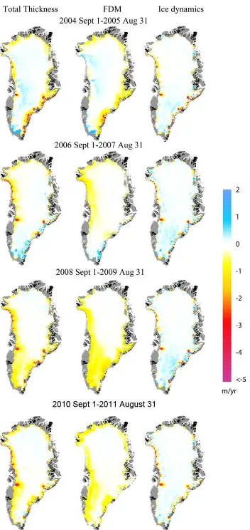
The new reconstruction improves the spatial resolution of previ-ous annual thickness change rate grids (Fig. 7). It is especially obvious along the SE coast of Greenland, where the local thin-ning and thickethin-ning patters are confined to individual drainage basins, rather than occur over larger regions as shown in earlier work (Csatho et al., 2014).
Figure 7. Annual total, FDM and ice dynamics related ice thick-ness changes in Greenland.
The annual ice sheet volume change rates determined from the new reconstruction are very similar to our previously published values (Csatho et al., 2014) for the period of the ICESat mission (Table 1). The fact that the increased spatial density of time series does not change the overall volume change rate suggests that the sampling provided by the ICESat ground tracks was adequate for ice sheet mass balance monitoring at the scale of the entire GrIS.
However, there is a relatively large difference (30 %) between the previously determined and revised 2003-2004 volume change rates. The first complete 30-day data acquisition phase of ICE-Sat started in September 2003. In our previously reconstruction, we have not extended the record back to 2003 September 1 for those time series that started later in 2003 September with an L2a observation. Therefore, the distribution of the annual rates for the 2003-2004 balance years was very sparse. Our new work has remedied this situation by extrapolating all time series with one month before the first and one month after the last observation.
Volume change (km3
/yr
balance year Csatho et al., 2014 This study difference
2003-04 -197 -282 30
2004-05 -321 -334 4
2005-06 -300 -299 0
2006-07 -288 -277 4
2007-08 -282 -266 6
2008-09 -277 -280 1
Table 1. Volume change rates of the entire GrIS during the ICE-Sat mission period from Csatho et al., 2014 and this study.
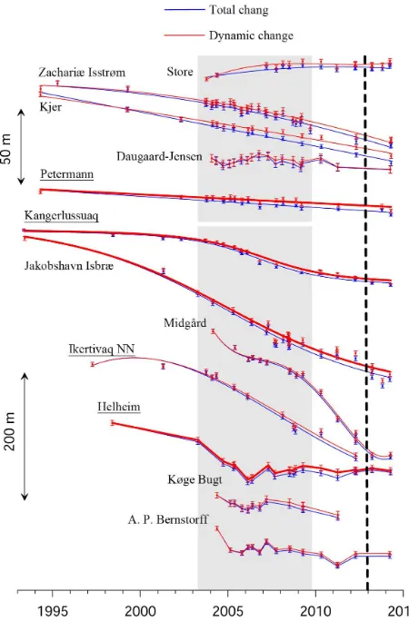
The extended time series of Greenland outlet glaciers indicates that outlet glacier behavior remained relatively unchanged during the 2012-2014 time period. Thus, glaciers that belong to the cate-gory according to the their ice thickness change patterns in 1993-2012 (Fig. 8), still exhibit similar behaviors (Fig. 9). For example Zacharyæ Isstrøm in NE Greenland has continued to accelerate in NE Greenland, while Kjer Glacier in W Greenland continues to thin with a uniform rate. However, after a short period of de-creasing thinning, Jakobshavn Isbræ has resumed rapid thinning after 2012. It is worth to note that the re-stabilization of Helheim, Køge Bugt and A.P. Barnstorm glaciers in SE Greenland appears to be complete as these glaciers show very little elevation change in the 2012-2014 period.
Figure 9. Thickness change time series (blue: total change, red dynamic change) derived from the combined ICESat/ATM/LVIS altimetry record (1993-2014) illustrating different dynamic outlet glacier behaviors.
4. CONCLUSION
We describe a new methodology which provides improved ca-pabilities of detecting and monitoring surface elevation changes over ice sheets and glaciers where elevation data are collected. We demonstrate the modular flexibility of the SERAC detection framework by applying different firn-densification and glacial iso-static adjustment models between the Greenland and Antarctic Ice Sheets to investigate the uncertainty of ice-sheet mass loss estimates derived from altimetry.
We show the first detailed reconstruction of annual dynamic ice thickness changes in Antarctica, generated on an observation-by-observation basis with quantified error estimates. We highlight regional complexity of dynamic ice thickness behavior in Antarc-tica for the Pine Island region as well as the Siple Coast, related to the stagnation of the Kamb Ice Stream and continued thinning of Mercer Ice Stream likely caused by long-term dynamic imbal-ance. We also illustrate the utility of SERAC to describe very lo-calized changes in ice dynamics, particularly those likely related to changes in subglacial hydrology or subglacial geology.
In Greenland, the large spatial and temporal variations of dy-namic mass loss and widespread intermittent thinning depicted by our annual elevation change rate maps indicate the complexity of ice sheet response to climate forcing, strongly enforcing the need for continued monitoring at high spatial resolution and for
im-proving numerical ice sheet models. Moreover, the sensitivity of the altimetry-based mass balance solutions to the applied climate models and corrections highlights the need for a synergistic ap-plication of different methods (gravimetry, GPS, altimetry, input-output method). While all of the results described in this work involved crossover-type solutions, efforts are currently underway to densify observations, in both Greenland and Antarctica, us-ing along-track solutions and by fusus-ing different sensor data with laser altimetry. Additionally, the modular SERAC framework should prove valuable in future ensemble-of-models approaches to examine the sensitivity of surface elevation changes to differ-ent models of glacial isostatic adjustmdiffer-ent, firn-densification, and sensor-based biases.
REFERENCES
Csatho, B. M., Schenk, A. F., van der Veen, C. J., Babonis, G., Duncan, K., Rezvanbehbahani, S., Van Den Broeke, M. R., Si-monsen, S. B., Nagarajan, S. and Van Angelen, J. H., 2014. Laser altimetry reveals complex pattern of Greenland Ice Sheet dynam-ics. Proceedings of the National Academy of Sciences111(52), pp. 18478–18483.
Haran, T., 2005. MODIS mosaic of Antarctica (MOA) image map. p. Retrieved from http://www.add.scar.org/index.jsp.
Hofton, M. A., Luthcke, S. B. and Blair, J. B., 2013. Estimation of ICESat intercampaign elevation biases from comparison of li-dar data in East Antarctica.Geophysical Research Letters40(21), pp. 5698–5703.
Kuipers Munneke, P., Ligtenberg, S. R. M., No¨el, B. P. Y., Howat, I. M., Box, J. E., Mosley-Thompson, E., McConnell, J. R., Stef-fen, K., Harper, J. T., Das, S. B. and Van Den Broeke, M. R., 2015. Elevation change of the Greenland Ice Sheet due to surface mass balance and firn processes, 1960–2014. The Cryosphere
9(6), pp. 2009–2025.
Ligtenberg, S., Helsen, M. and Van Den Broeke, M. R., 2011. An improved semi-empirical model for the densification of Antarctic firn.The Cryosphere5(4), pp. 809–819.
Rastner, P., Bolch, T., M¨olg, N., Machguth, H., Le Bris, R. and Paul, F., 2012. The first complete inventory of the local
glaciers and ice caps on Greenland. The Cryosphere 6(6), pp. 1483–1495.
Schenk, T. and Csatho, B., 2012. A new methodology for detect-ing ice sheet surface elevation changes from laser altimetry data.
Geoscience and Remote Sensing, IEEE Transactions on50(9), pp. 3302–3316.
Sergienko, O. V. and Hulbe, C. L., 2011. ’Sticky spots’ and sub-glacial lakes under ice streams of the Siple Coast, Antarctica. An-nals of Glaciology52(58), pp. 18–22.
Siegfried, M. R., Hawley, R. L. and Burkhart, J. F., 2011. High-resolution ground-based GPS measurements show inter-campaign bias in ICESat elevation data near Summit, Greenland.
Geoscience and Remote Sensing, IEEE Transactions on49(9), pp. 3393–3400.
Van Der Veen, C. J., Ahn, Y., Csatho, B. M., Mosley-Thompson, E. and Krabill, W. B., 2009. Surface roughness over the north-ern half of the Greenland Ice Sheet from airborne laser altimetry.
Journal of Geophysical Research114(F1), pp. F01001. The International Archives of the Photogrammetry, Remote Sensing and Spatial Information Sciences, Volume XLI-B8, 2016
Van Der Veen, C. J., Krabill, W. B., Csatho, B. M. and Bolzan, J. F., 1998. Surface roughness on the Greenland ice sheet from airborne laser altimetry. Geophysical Research Letters25(20), pp. 3887–3890.
van Meijgaard, E., Van Ulft, L., van de Berg, W., Bosveld, F., Van den Hurk, B. J. J. M., Lenderink, G. and Siebesma, A., 2008. The KNMI regional atmospheric climate model RACMO. ver-sion 2.1. Tech. Rep. TR-302, Royal Netherlands Meteorological Institute.
Whitehouse, P. L., Bentley, M. J., Milne, G. A., King, M. A. and Thomas, I. D., 2012. A new glacial isostatic adjustment model for Antarctica: calibrated and tested using observations of rela-tive sea-level change and present-day uplift rates. Geophysical Journal International190(3), pp. 1464–1482.