Econometrics
Jeffrey M. Wooldridge
Wooldridgeabstract
This paper provides an overview of control function (CF) methods for solving the problem of endogenous explanatory variables (EEVs) in linear and nonlinear models. CF methods often can be justifi ed in situations where “plug- in” approaches are known to produce inconsistent estimators of parameters and partial effects. Usually, CF approaches require fewer assumptions than maximum likelihood, and CF methods are computationally simpler. The recent focus on estimating average partial effects, along with theoretical results on nonparametric identifi cation, suggests some simple, fl exible parametric CF strategies. The CF approach for handling discrete EEVs in nonlinear models is more controversial but approximate solutions are available.
I. Introduction
The term “control function” has been part of the econometrics lexicon for several decades, but it has been used inconsistently, and its usage has evolved. In early work—notably, Barnow, Cain, and Goldberger (1981) (hereafter, BCG)—a con-trol function is a variable that, when added to a regression, renders a policy variable appropriately exogenous. From the BCG perspective, multiple regression that includes the policy variable and one or more control functions provides consistent estimation of the causal effect of a policy intervention. Cameron and Trivedi (2005, p. 37) en-dorses this defi nition of a control function (CF), and, based on the usage in BCG, what Wooldridge (2010, Section 4.3.2) defi nes as a proxy variable would be considered a CF. As one example, a standardized intelligence test score, such as IQ score, can be considered a CF if conditioning on it appropriately controls for unobserved cognitive ability, thereby enabling consistent estimation of the causal effect of schooling in a standard wage equation.
Jeffrey M. Wooldridge is a University Distinguished professor of economics at Michigan State University. He thanks four anonymous referees and the editors for very helpful comments on two earlier drafts. Data used in this article are available from the author from November 2015 through October 2018.
[Submitted April 2013; accepted February 2014]
ISSN 0022- 166X E- ISSN 1548- 8004 © 2015 by the Board of Regents of the University of Wisconsin System
In the application motivating BCG, variables measuring socioeconomic status (SES) are control functions if participation in a program—such as Head Start—is essentially determined by the SES variables. Goldberger (1972, reprinted 2008) was an important contribution studying the problem of whether controlling for observables could solve self- selection into program participation although it did not use the phrase “control function.” Therefore, in early usage, the notion of a control function was closely tied to assumptions of “ignorable” or “unconfounded” treatment assignment that are prevalent today: Conditional on observed covariates, the key policy variables are appropriately exogenous. (For an overview, see Imbens and Wooldridge 2009.)
Heckman and Robb (1985), in the context of program evaluation with longitudinal data, also describes a control function as a variable that, when conditioned on, makes an intervention exogenous in a regression equation. It explicitly recognizes that CFs might depend on unknown parameters and that to operationalize a CF procedure the parameters must be estimated in a fi rst stage. One example is a lagged residual in a program evaluation equation using longitudinal data.
For the most part, the modern usage of “control function” maintains the spirit of the earlier defi nitions but with an important defi ning feature: Constructing a valid CF relies on the availability of one or more instrumental variables. I take this perspective in the current paper: The control function approach to estimation is inherently an instrumental variables method. More precisely, the equation of interest—for brevity called the “struc-tural equation”—contains at least one explanatory variable that is endogenous, or sus-pected of being so, in the sense that it is correlated with unobservables in the equation. Further, I have excluded exogenous variables from the structural equation that explain variation in the endogenous explanatory variables (EEVs for short). The exogenous variation induced by excluded instrumental variables provides separate variation in the residuals (or generalized residuals) obtained from a reduced form, and these residuals serve as the control functions. By adding appropriate control functions, which are usually estimated in a fi rst stage, the EEVs become appropriately exogenous in a second- stage estimating equation. The purpose of this review is to show how this general description of the CF approach can be applied to various linear and nonlinear models.
In evaluating the scope of an estimation method, it is important to understand how it works in familiar settings, including cases when it is not necessarily needed. Conse-quently, in Section II, I discuss the control function approach applied to linear models with constant coeffi cients. Such models are still the workhorse in applied econometrics, and simple IV methods, such as two- stage least squares (2SLS), are usually suffi cient for estimation. Nevertheless, even when the CF approach is identical to a 2SLS estima-tor, the CF perspective has a couple of attractive features. First, the CF approach pro-duces a simple Hausman (1978) test that compares OLS and 2SLS, and the test is easily made robust to heteroskedasticity and cluster correlation (including serial correlation in a panel data setting) of unknown form. Second, the CF approach parsimoniously handles fairly complicated models that are nonlinear in endogenous explanatory variables.
stan-dard IV methods under general assumptions, with the “local average treatment effect” (LATE) introduced in Imbens and Angrist (1994) being the most popular.
I argue in Section III that the control function approach is a useful complement to stan-dard IV methods for a couple of reasons. First, we might hope to estimate treatment effects for identifi able populations or subpopulations, and the CF approach allows us to do that under certain assumptions. Second, the CF approach allows us to study the nature of self- selection. In particular, if we think units self- select into treatment when the treatment is likely to be benefi cial, then we should be able to test that proposition. A classic example is the endogenous switching regression model, as in Heckman (1976), which is often applied to earnings equations under two different regimes (such as belonging to a union or not).
I discuss estimation of nonlinear models in Section IV, where the CF approach is par-ticularly appealing compared with other approaches such as “plug- in” methods or joint maximum likelihood. Important contributions are Rivers and Vuong (1988), which de-veloped a two- step CF method for estimation of a probit model with a continuous EEV, and Smith and Blundell (1986), which essentially did the same for the Tobit model. In these early applications of CF methods to nonlinear models, the focus was on parameter estimation. Many of the recent advances in CF methods demonstrate that average par-tial effects, or average causal effects, are identifi ed quite generally. Wooldridge (2010) uses these results extensively and, in pioneering work, Blundell and Powell (2003) shows that the concept of a control function can be applied in nonparametric and semi-parametric contexts. For discrete EEVs, I also summarize the CF methods recently proposed by Terza, Basu, and Rathouz (2008) and Wooldridge (2014). These methods are more controversial because they rely on nonstandard parametric assumptions.
To illustrate several of the CF methods, I present applications to three data sets. One data set allows estimation of a log wage equation allowing for education to be endogenous. Such equations can be estimated assuming a constant return to education, as in Section II, or the return to education can be individual- specifi c, as in Section III. A second application is to a math test score equation, where the EEV of interest is a binary indicator of attending a Catholic high school. Again, one can assume constant coeffi cients or allow the effect of attending a Catholic high school to depend on un-observed characteristics. As we will see in Section III, there is strong evidence for individual- specifi c heterogeneity in the effects of attending a Catholic high school.
To illustrate nonlinear models in Section IV, I use a data set on married women’s labor force participation, where the variable measuring other sources of income is treated as endogenous. I show how to estimate the simple Rivers- Vuong model and also show how the CF approach can be made much more fl exible with almost no addi-tional computation. Finally, I briefl y consider a binary response model for graduating from high school with attending a Catholic high school as the endogenous explanatory variable. The data sets and Stata® code used for all models estimated in the paper are available on request from the author.
II. Models Linear in Constant Coef
fi
cients
control function (CF) approach leads to robust, regression- based Hausman tests of whether the suspected EEVs are actually endogenous. Third, the basic 2SLS approach can be contrasted with CF approaches that put structure on the reduced forms of the endogenous explanatory variables. CF approaches that use more information can im-prove precision of the estimates but are generally less robust.
I consider a setting where y1 is a scalar response variable, y2 is the endogenous ex-planatory variable (also a scalar for simplicity), and z is the 1× L vector of exogenous variables, which I assume contains unity to allow for a nonzero intercept. The “struc-tural” equation in the population is
(1) y1= z
1␦1+␥1y2+u1,
where z1 includes unity and is a 1×L1 subvector of z = (z1, z2). The sense in which z is exogenous is given by the L orthogonality (zero covariance) conditions
(2) E(z′ju1)=0, j=1, 2, ...,K.
The assumptions in Equation 2 hold if I make the stronger assumption E(u1|z)= 0,
which is sometimes preferred if Equation 1 is supposed to be a structural equation— but I fi rst derive the CF approach under the same assumption employed by 2SLS, which is Equation 2.
I make the standard assumption that the elements of z are not perfectly collinear. In addition, I assume the rank condition for identifi cation holds. In the context of Model 1, the rank condition is most easily stated in terms of the linear reduced form for y2. If I write
(3) y2= z2+v2= z121+z222+v2
(4) E(z′v
2)= 0,
then the rank condition holds if and only if 22 ≠ 0. This is just the usual requirement that there be at least one exogenous variable that is omitted from Equation 1 that is partially correlated with y2. As is now widely appreciated, given a random sample, one should estimate the reduced from in Equation 3 and be able to reject the null H0:22 = 0 at a suitably small signifi cance level.
A leading example of the above setup is when y1 is the logarithm of hourly earn-ings, y2 is a measure of schooling, and z1 includes other determinants of wages that are assumed to be exogenous (such as workforce experience). Many instrumental variables have been proposed for schooling in the literature, ranging from parents’ education to quarter of birth; Card (2001) includes a survey of some of the more convincing efforts.
As a second example, suppose y1 is performance on a standardized test and y2 is a binary indicator of attending a Catholic high school, a problem studied by Altonji, El-der, and Taber (2005), among others. In thinking about the scope of the model in Equa-tion 1, it is important to understand that it allows for y2 to be continuous or discrete (or some mixture). The linear reduced form in Equation 3 under Condition 4 can always be specifi ed regardless of the nature of y2. I need provide no structural interpretation of this equation. I simply need z2 to be correlated with y2 after partialling out z1.
(5) u1=1v2+e1
(6) E(v2e1)=0,
where 1= E(v2u1) / E(v22) is the population regression coef
fi cient. Because u1 and v2 are uncorrelated with z, it follows that e1 is also uncorrelated with z, and then e1 must also be uncorrelated with y2. Therefore, I obtain a valid estimating equation by plug-ging Equation 5 into the structural equation to get
(7) y1= z
1␦1+␥1y2+1v2+e1.
In the CF approach, one views v2 as an explanatory variable in Equation 7. By including it, one obtains a new error term, e1, that is uncorrelated with all other righthand- side vari-ables, including y2. In effect, including v2 in the equation “controls for” the endogeneity of y2. One can think of v2 as proxying for the factors in u1 that are correlated with y2.
A. Control Function Procedure: Linear Reduced Form
If one could observe v2 along with the other variables, Equation 7 immediately sug-gests a way to estimate ␦1, ␥1, and 1: Run the OLS regression of yi1 on zi1, yi2, and vi2 using a random sample of size N. The only problem is that one does not observe v2. Nevertheless, from Equation 3, one can write v2 = y2−z
2 and, because data is col-lected on y2 and z, one can consistently estimate 2 by OLS. This leads to the follow-ing two- step control function procedure:
1. Run the OLS regression of the EEV, yi2, on all exogenous variables, zi,
(8) yi2 on z
i, i=1, ...,N
and obtain the OLS residuals, vˆi2. 2. Run the OLS regression
(9) yi1 on z
i1, yi2, ˆvi2, i=1, ...,N
to obtain ␦ˆ1, ␥ˆ1, and ˆ1.
It has been known since at least Hausman (1978) that this CF method produces coeffi -cients on zi1 and yi2 that are numerically identical to the 2SLS estimates. Therefore, one might wonder what all the fuss is about. It is true that, in this particular setting, the CF approach does not lead to a new estimator. In fact, obtaining proper standard errors from the regression in Equation 9 is made diffi cult by the fi rst- stage estimation of 2. Neverthe-less, compared with the 2SLS approach, the inclusion of vˆi2 serves a valuable purpose: It produces a heteroskedasticity- robust Hausman test of the null hypothesis H0 : 1=0, which means y2 is actually exogenous. The traditional form of the Hausman test that di-rectly compares OLS and 2SLS is substantially harder to make robust to heteroskedasticity. The importance of the identifi cation requirement that 22 ≠0 can be seen by study-ing Equations 3 and 7. If 22 =0, then v2 is a linear function of y2 and z1, which means v2 is collinear in Equation 7. The presence of z2 that is partially correlated with y2 en-sures v2 has variation separate from (z1, y2). If there are no variables z2 then the CF regression in Equation 9 suffers from perfect multicollinearity in the sample, and esti-mates of all parameters cannot be produced. These same observations apply to more complicated CF procedures covered later.
the return to schooling in Card (1995) and the other a subset of the data on student performance and Catholic school attendance from Altonji, Elder, and Taber (2005) (hereafter, AET). In both cases, the authors provide detailed discussions about the exogeneity of the instruments, and AET casts doubt on the exogeneity of a commonly used distance instrument. Nevertheless, I proceed as if the instruments are exogenous.
I begin with a standard wage equation
lwage =z1␦1+␥1educ+u1,
where lwage is the log of wage and z1 contains exogenous variables and a constant. Years of schooling, educ, can be correlated with u1 for many reasons, such as omitted ability and measurement error. Rather than estimate ␥1 by OLS, I can try to fi nd one or more instrumental variables for educ. Card (1995) uses two dummy variables indicat-ing whether there is a two- year college (nearc2) or four- year college (nearc4) in the local labor market at age 16. Details of the data are described in Card (1995).
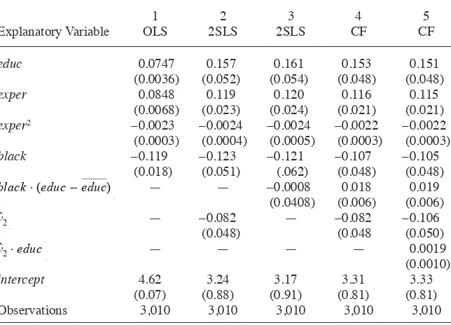
Table 1 reports several estimates. The fi rst column contains the OLS estimates with the controls used in Card (1995). The return to a year of schooling is estimated to be Table 1
Notes: (i) Each equation contains dummy variables for living in an SMSA and living in the South. In addition, they include regional dummies for where the man was living in 1966 and an indicator of whether the man lived in an SMSA in 1966.
(ii) Standard errors for OLS and 2SLS are robust to heteroskedasticity. (iii) In Column 2, the 2SLS estimates are equivalent to the CF estimates.
0.075 (t = 20.48). Column 2 contains the 2SLS estimates reported in control function form with the reduced form residual included. The heteroskedasticity- robust tstatistic on vˆ2 is –1.72, which is a marginal rejection of the null that education is exogenous—
even though the 2SLS point estimate for the return to education (0.157, t = 3.00) is much higher than the OLS estimate.
For the AET application, I estimate the model
math12 = z1␦1+␣1cathhs+u1,
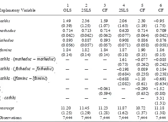
where z1 includes an intercept, mother’s education, father’s education, and the log of family income. The instruments for cathhs, which is a binary indicator for attending a Catholic high school, is distance from the nearest Catholic high school divided into fi ve bins. Thus, four distance dummies are used as IVs for cathhs. The OLS and 2SLS estimates are given in Columns 1 and 2 of Table 2. The OLS estimate on cathhs is about 1.49 (t = 3.84), or about 0.16 standard deviations in the test score. The 2SLS estimate is 2.36 (t = 1.90). However, the heteroskedasticity- robust test statistic on the Table 2
Estimates of the math12 Equation
Explanatory Variable
Notes: (i) Standard errors for OLS and 2SLS are robust to heteroskedasticity. (ii) The standard errors for the CF estimates are based on 1,000 bootstrap replications.
control function (not reported in the table) is only t = –0.75, so the OLS and 2SLS estimates are not statistically different.
B. Exploiting a Binary EEV
The test score example raises an interesting question because the EEV, cathhs, is bi-nary. The standard IV approach treats all EEVs the same: The structural equation is supplemented with the linear reduced form given in Equations 3 and 4. An alternative is to recognize the binary nature of y2 and replace its linear reduced form with a binary response model. The two equations are then
(10) y1=z1␦1+␥1y2+u1
(11) y2 =1[z␦2+e2>0],
where 1[⋅] is the binary indicator function. With these equations, one would assume that (u1, e2) is independent of z, which is already much stronger than the zero correla-tion assumpcorrela-tions used by the previous CF (2SLS) estimator. If it is assumed that u1 is linearly related to e2 and that
(12) e2∼ Normal(0,1),
then one can derive an alternative control function method. An implication of Equa-tions 11 and 12 is that y2 follows a probit model:
(13) P(y2=1|z)=⌽(z␦2),
where ⌽(⋅) is the standard normal cumulative distribution function. Nothing was as-sumed of the sort to apply 2SLS to Equation 1.
A thorough understanding of the pros and cons of different CF approaches requires one to understand that the model for y2 in Equations 11 and 12 is entirely compatible with the linear reduced form defi ned by Equations 3 and 4. The usual 2SLS approach assumes nothing about the distribution of y2 given z. By contrast, Equations 11 and 12 completely characterize the distribution of y2 given z.
C. Control Function Procedure: Probit Reduced Form
When one specifi es a full distribution for y2, the CF approach is based on the conditional expectation E(y1|z,y2). This is a subtle difference with the 2SLS ap-proach, which is based on zero correlation assumptions only. It is well known— see, for example, Wooldridge (2010, Section 21.4.2)—that under the previous as-sumptions,
(14) E(y1|z,y2)= z1␦1+␥1y2+1[y2(z␦2)−(1− y2)(−z␦2)],
where (⋅)=(⋅) /⌽(⋅) is the well- known inverse Mills ratio. The function
(15) r(y2,z␦2)≡ y2(z␦2)−(1− y2)(−z␦2)
1. Estimate the probit model in Equation 13. Obtain the “generalized residuals”
(16) rˆi2≡ yi2(zi␦ˆ2)−(1− yi2)(−zi␦ˆ2), i=1, ...,N.
2. Run the OLS regression
(17) yi1 on zi1, yi2, ˆri2, i =1, ...,N
to consistently estimate ␦1, ␥1, and 1.
As with the fi rst CF approach—the one that produces 2SLS—a simple test of the null hypothesis that y2 is exogenous is obtained as the (heteroskedasticity- robust) t statistic on rˆi2.
The CF approach from Regression 17 is the same one computed by the “treatreg” command in Stata® using its two- step option. It exploits the binary nature of y
2 but not without cost. For one, it is generally inconsistent if the probit model for y2 is misspecifi ed. This is in contrast to the usual 2SLS estimator—equivalently, the CF estimator from Equation 9. The robustness of the 2SLS estimator compared with the estimator from Equation 17 is perhaps counterintuitive and has generated some confu-sion among empirical researchers. The key is that 2SLS does not use any distributional assumptions in the reduced form whereas the expression in Equation 14 does. If the probit model for y2 is correctly specifi ed, then the CF procedure in Equation 17 and 2SLS should give estimates that differ only due to sampling error.
Column 3 in Table 2 contains the CF estimates obtained from Equation 17 for the math12 equation. The cathhs coeffi cient is 1.59, which is close to the OLS estimate. This is expected because the t statistic on rˆi2 is only –0.10. If the coeffi cient on the generalized residual were statistically signifi cant, one should adjust the standard errors for the two- step estimation. The bootstrap can be used if analytical methods are not readily available. Given the three estimates so far—OLS, 2SLS (the CF estimates from Equation 9), and the CF estimates from Equation 17—there is no reason to reject the OLS estimate. This is not the case when one turns to a richer set of models.
D. Models Nonlinear in the EEV
One benefi t of the CF approaches in Equations 9 and 17 is that they are easily adapted to handle more complicated models. As one important example, consider a model where y2 interacts with the exogenous variables (and appears on its own because z1 includes an intercept):
(18) y1=z1␦1+ y2z1␥1+u1.
If y2 is continuous, then one can use the regression in Equation 9 where yi2zi1 replaces yi2, which means yi2 appears on its own and interacted with exogenous variables. If yi2 is binary, then one uses Regression 17, where yi2 appears by itself and interacted with exogenous variables. The t statistic on either vˆi2 or rˆi2, perhaps made robust to hetero-skedasticity, is still a valid test of the null that y2 is exogenous. Because Equation 18 contains only a single EEV, a one degree- of- freedom test is appealing.
where ⌽(zi␦ˆ2) are the probit fi tted values. This IV estimator has a theoretical
advan-tage over the CF estimator, at least if one assumes the linear model with constant coef-fi cients is the correct specifi cation: The IV estimator is generally consistent even if the probit model is misspecifi ed. Thus, one can exploit the binary nature of y2 but still obtain an estimator that does not require a correctly specifi ed model for D(y2|z), the
distribution of y2 given z. However, the CF approach offers a parsimonious way to account for endogeneity of y2 even if it interacts with many exogenous variables. It seems likely that it is more effi cient quite generally, but this possibility seems not to have been systematically investigated.
In Columns 3 and 4 of Table 1, I include an interaction between the race indicator, black, and educ, where I fi rst center educ about its mean (roughly 13.3) before creat-ing the interaction. Column 3 contains the 2SLS estimates where nearc2, nearc4, black⭈nearc2, and black⭈nearc4 are used as instruments for educ and black⭈ (educ – educ). The coeffi cient on the latter is –0.0008, which is small and has a very wide 95 percent confi dence interval. Column 4 contains the CF approach, and now the coef-fi cient on the interaction term is positive and practically large, 0.018, and statistically signifi cant with t = 2.84. The return to education is estimated to be about 1.8 percent-age points higher for black men. Further, the earnings gap between black and nonblack men shrinks at high levels of education. The picture given by the CF estimates is dif-ferent from the much less precise 2SLS estimates.
In the test score equation, I interact cathhs with motheduc, fatheduc, and lincome. Column 4 in Table 2 contains the estimates where the fi tted probit probabilities and interactions are used as IVs, while Column 5 contains the CF estimates from add-ing the generalized residual. The estimates are notably different. The CF estimate of the average effect of cathhs is 2.30 (t = 1.94) and the interaction terms are all small and insignifi cant (although the interaction with lincome has t = –1.79). By contrast, the average effect estimated by 2SLS is insignifi cant but there appears to be a large, statistically signifi cant interaction with mother’s education. I cannot reconcile the dif-ference in these estimates without allowing the treatment effect of cathhs to depend on unobservables, which I do in the next section.
Before ending this section, it is useful to summarize the key points of how the CF approach compares with other common approaches.
1. In the basic linear model with constant coeffi cients, where the EEV appears lin-early, and where I use linear reduced forms, the CF approach is the same as 2SLS. The CF approach provides a simple, robust test of the null hypothesis that y2 is exogenous.
2. When I exploit special features of the EEV y2—for example, recognize that it is a binary variable—the CF approach uses generalized residuals. The CF approach is likely more effi cient than 2SLS because it exploits the binary nature of y2 but, in terms of consistency, the CF approach is usually less robust than IV approaches.
III. Correlated Random Coef
fi
cient Models
The setup of the previous section allows the endogenous explanatory variable or variables to appear linearly or nonlinearly and to interact with observed covariates. This may be suffi cient for some applications, but one may also want to allow the effect of y2 to depend on unobservables. One might think, for example, that the return to schooling or the causal effect of attending a Catholic high school vary across individuals in ways that cannot be observed fully. When one allows random coeffi cients to be correlated with some explanatory variables, such as amount of school or choice of school, one obtains a “correlated random coeffi cient” (CRC) model, a label adopted by Heckman and Vytlacil (1998) and discussed in the context of the return to schooling by Card (2001). In the treatment effects literature, CRC models allow for heterogeneous treatment effects combined with self- selection into treatment—provided that there are suitable instrumental variables for treatment as-signment.
Consider the problem of estimating a wage equation with an individual- specifi c return to schooling. For a random draw i,
(19) lwagei= zi1␦1+gi1educi+ui1,
where gi1 is the individual- specifi c return to schooling. Now there are two sources of unobserved heterogeneity and both gi1 and ui1 might be correlated with educi. In fact, due to self- selection, one might expect the amount of education, educi, to be positively correlated with gi1: people for whom the return to schooling is higher will choose, on average, to obtain more education.
Certainly, one cannot expect to estimate gi1 for each i. Instead, I focus on the aver-age return to schooling in the population, ␥1= E(gi1). Then I can write gi1= ␥1+vi1 where E(vi1)=0. Plugging into Equation 19 gives
(20) lwagei= zi1␦1+␥1educi+vi1educi+ui1.
If I apply the usual 2SLS estimator to Equation 20, then the error term is implicitly
ei1=vi1educi+ui1. As discussed in Wooldridge (2003), the 2SLS estimator is generally inconsistent for ␥1, although it is consistent if one assumes, in addition to the standard exogeneity requirements
(21) E(ui1|zi)=0, E(vi1|zi)=0,
a constant conditional covariance assumption:
(22) Cov(educi,vi1|zi)=Cov(educi,vi1).
Notice that Condition 22 allows arbitrary correlation between educi and the random re-turn to education, gi1. But the conditional covariance cannot depend on the exogenous variables. Card (2001) discusses situations where this assumption is likely to fail in simple models of schooling decisions.
(23) yi2 =zi2+vi2, E(vi2|zi)=0.
Assume also that both sources of unobservables, ui1 and vi1, are linearly related to vi2:
(24) E(ui1|vi2)=1vi2, E(vi1|vi2)= 1vi2
and that all unobservables are independent of zi. The estimating equation is
(25) E(yi1|zi,yi2)= E(yi1|zi1,yi2,vi2)= zi1␦1+␥1yi2+1vi2+1vi2yi2.
Equation 25 leads to the following simple CF approach. As before, estimate Equation 23 by OLS and obtain the residuals, vˆi2. Second, run the OLS regression
(26) yi1 on zi1, yi2, ˆvi2, ˆvi2yi2, i=1, ...,N.
Compared with the constant- coeffi cient case, I have added the interaction term ˆ
vi2yi2. Without the interaction, I know that Regression 26 produces the 2SLS estimates of ␦1 and ␥1. The interaction term accounts for the random coeffi cient on yi2. It is of interest to test for statistical signifi cance of the interaction term, but one must be care-ful: If the coeffi cient on vi2 is different from zero, the usual t statistic on yi2vˆi2 is not valid because of the fi rst- stage estimation. It is simple to bootstrap the two- step pro-cedure to obtain valid standard errors for all of the coeffi cients. Conveniently, a test of joint signifi cance of ( ˆvi2, ˆvi2yi2) is valid without adjusting the standard errors. The joint test is a test of the null hypothesis that y2 is exogenous.
Given the results on 2SLS by Wooldridge (2003) described earlier, it is possible that the coeffi cient on vˆi2yi2, ˆ1, is large and statistically signifi cant but the estimate of ␥1 is similar to the 2SLS estimate. Even if the two procedures give similar estimates of the average effect, ˆ1 is of some interest because one can write
(27) E(gi1|vi2)=␥1+1vi2.
Even though I cannot estimate gi1, I can estimate its expected value given the reduced form error, vi2, which necessarily has a zero mean. In the return- to- schooling example, I might expect 1>0 because, as vi2 increases, the person has more education than is predicted by the exogenous variables, zi. A positive 1 is consistent with a selection story: conditional on zi, people obtain more education if their return to schooling is higher. One can estimate the righthand side of Equation 27 as ␥ˆ1+ˆ1vˆi2 for each i and, if desired, study how these estimates vary across i. The average of the individual par-tial effects in the sample is, mechanically, ␥ˆ1.
As with the simpler CF method from Section II, Regression 26 easily extends to allow any nonlinear functions of (zi1, yi2), including quadratics and interactions. I estimate the wage equation using the Card (1995) data by including the interaction blacki⭈ (educi – educ) along with vˆi2 and vˆi2⋅educi; the results are in Column 5 of Table 1. The estimates on the educi, blacki, and blacki⭈ (educi – educ) are similar to the CF estimates without the interaction term vˆi2⋅educi, even though the latter is marginally signifi cant (t = 1.84), re-vealing a certain robustness of the simpler CF approach. (Jointly, vˆi2 and vˆi2⋅educi are signifi cant with p–value = 0.042). From Equation 27, the positive coeffi cient on vˆi2⋅educi implies that those with higher- than- predicted education have, on average, higher returns to schooling, thereby providing some evidence for self- selection into schooling.
analysis is obtained by choosing a 1×K1 set of regressors, xi1, to be any function of (zi1, yi2), say g1(zi1, yi2). This can include, in addition to zi1 and yi2, terms such as yi2
2 and
zi1yi2, or even higher order polynomials and interactions. If one separates out an inter-cept and allow all K1 elements of xi1 to have random slopes b to use the nonparametric bootstrap, where both estimation steps are included, to obtain valid inference. If ˆ1 is the K1 vector of OLS coeffi cients on x
i1vˆi2, one can estimate E(b
i1|vi2) as ˆ1+vˆi2ˆ1 and possibly provide economic interpretations for the signs and magnitudes of the elements of ˆ1.
Even more fl exibility is obtained by allowing E(v
i1|vi2) to be a nonlinear function in
2 is the usual OLS variance estimate from the
fi rst stage, get added to Equation 29. It is evident that these extensions of Garen’s (1984) CF ap-proach allow signifi cant fl exibility in correlated random coeffi cient models.
The CF approach can also be used to estimate the random coeffi cient model when y2 is binary. The typical endogenous switching model is
(30) yi1= ␣1+zi1␦1+␥1yi2+ yi2zi11+ui1+yi2vi1
and I combine this with the probit model for y2, given in Equations 11 and 12, with all unobservables independent of zi. After obtaining the generalized residuals in Equation 16, the CF regression is
(31) yi1 on 1, zi1, yi2, yi2⋅(zi1−z1), ˆri2, yi2rˆi2,
where, again, centering zi1 about the sample averages ensures that the coeffi cient on yi2 is the average effect.
The estimates of the switching regression model for the test score data are given in Column 6 of Table 2. These estimates provide a very different picture than either the 2SLS estimates or the CF estimates that ignore the random coeffi cient on cathhsi. First, the two terms rˆi2 and cathhsi⋅rˆi2 are jointly signifi cant using a heteroskedasticity- robust test with p–value = 0.022. By contrast, when rˆi2 is included by itself, its t statis-tic is only –0.46. The coeffi cient on cathhsi⋅rˆi2 is very large, 3.31 with t = 2.53, pro-viding evidence that the treatment effect of attending a Catholic high school depends strongly on unobserved heterogeneity. Even more importantly, the average treatment effect in the population is now negative and not statistically different from zero:
ˆ
␥1=−0.95, (t = –0.58).
estimate is the average treatment effect for those who are induced to attend a Catholic high school because they live near a Catholic high school. This subpopulation can be very different from the overall population, where the effect estimated by the CF ap-proach is not statistically different from zero.
One can shed further light on the difference between the 2SLS and CF estimates by computing the average treatment effect on the treated (ATT) and the average treatment effect on the untreated (ATU); see Imbens and Wooldridge (2009). The simplest way of obtaining these quantities is to estimate separate equations for the control (yi2 = 0) and treated (yi2 = 1) groups, in each case by regressing yi1 on 1, zi1, rˆi2. Then, fi tted values from each regression are obtained for all observations i, say yˆi1(0) and yˆi1(1), respectively. Then
(32) pATT = N1−1 i=1
N
∑
yi2[ ˆyi1(1)−yˆi1(0)],which is simply the average in the difference of fi tted values over the yi2 = 1 observa-tions. (See, for example, Heckman, Tobias, and Vytlacil 2003.) Similarly, ATUp is the average of yˆi1(1)− yˆi(0)1 over the yi2 = 0 observations. Using the full endogenous switch-ing specifi cation, the estimated ATT (based on 452 students) is about 3.99 (t = 2.96). By contrast, the estimated ATU (based on 6,992 students) is about –1.27 (t = –0.73). The large difference is another way to illustrate the self- selection into attending a Catholic school: Those who would benefi t based on factors unobserved to us are much more likely to attend a Catholic high school. The usual 2SLS estimation of a linear model is necessarily silent on such selection issues because it only estimates the LATE.
The CF regression in Equation 31 can be made even more general to allow random coeffi cients on some or all of the exogenous variables as well as on the interaction terms. If one takes the vector of explanatory variables to be x
i1=(zi1,yi2,zi1yi2) and allow randomness in all coeffi cients b
i1, then the CF regression (across all observa-tions) becomes
(33) yi1 on 1, z
i1, yi2, yi2⋅(zi1−z1), ˆri2, yi2rˆi2, ˆri2⋅(zi1−z1), yi2⋅rˆi2⋅(zi1−z1).
The coeffi cient on yi2 in this regression is consistent for the average treatment effect. Alternatively, one can run separate regressions for the control and treated groups, where the regressions have the form yi1 on 1, zi1, rˆi2, and rˆi2z
i1. The estimated ATT is still obtained as in Equation 32, but the fi tted values are obtained by adding the terms rˆi2z
i1 to the separate regressions. As usual, bootstrapping is an attractive way to obtain valid standard errors. In the Catholic high school example, the expanded regression gives the following estimates (not reported in Table 2): ATTp =3.59(t = 2.62), ATUp =0.063 (t = 0.03), and ATEp =0.28 (t = 0.14). Thus, the picture is similar to the switching re-gression model with constant coeffi cients: The average treatment effect in the entire population is essentially zero, with a large average treatment effect for the relatively small treated subpopulation.
y1 is the log of wage or a test score, but linearity is harder to justify if y1 is discrete or its range is otherwise restricted. I now turn to nonlinear models for y1.
IV. Nonlinear Models
Control function methods have long been employed for particular non-linear models, especially probit and Tobit, when the endogenous explanatory variables are continuous. Thanks largely to the work of Blundell and Powell (2003, 2004), the scope of such applications is now much broader. Wooldridge (2005) and Petrin and Train (2010) give several examples of where CF methods can be applied with continu-ous EEVs. Here, I cover some simple examples that illustrate the fl exibility of the CF approach.
A. Continuous EEVs
Probably the leading example of a nonlinear model with continuous EEVs is the probit model, as analyzed in Rivers and Vuong (1988). With a single EEV y2, the model can be written as
(34) y1=1[z1␦1+␥1y2+u1≥0]
(35) y2= z␦2+v2,
where (u1, v2) is bivariate normal with mean zero, Var(u1) = 1, and independent of z. Here, both z and z1 include constants with z1, a strict subset of z. In most cases, the parameters of interest are constant insofar as they index partial effects. As discussed in Wooldridge (2010, Section 15.7.2), the average partial effects are obtained by taking derivatives or changes of
(36) Eui
1{1[z1␦1+␥1y2+ui1≥0]}=⌽(z1␦1+␥1y2), where the notation Eui
1{⋅} indicates averaging out the unobservables and treating (z1, y2) as fi xed arguments. Equation 36 is an example of what Blundell and Powell (2003) calls an “average structural function,” or ASF. In defi ning the ASF, the observables are taken as fi xed arguments and the unobservables are averaged out. Under the assump-tions given, the parameters in Equaassump-tions 34 and 35 and those in the bivariate normal distribution can be estimated using joint MLE, and so the ASF can be estimated as ⌽(z1␦ˆ1+␥ˆ1y2).
For the purposes of the current paper, a control function approach is attractive. The CF approach is based on the following conditional probability; see Wooldridge (2010, Section 15.7.2):
(37) P(y1=1|z,y2)= P(y1=1|z1,y2,v2)=⌽(z1␦1+␥1y2+1v2),
where E(u1|v2)=1v2, the subscript denotes division by (1−1 2
2
2)1/ 2, and 2 2
on zi1, yi2, vˆi2. The null hypothesis that y2 is exogenous is easily tested using the usual t statistic on vˆi2.
The CF approach appears to have the drawback that it does not estimate the param-eters ␦1 and ␥1 appearing in Equation 36. Fortunately, it turns out that the ASF is easily estimated using the scaled parameters identifi ed by Equation 37. As discussed in Wooldridge (2010, Section 15.7.2), the ASF can be obtained as
(38) ASF(z
1,y2)= Evi2[⌽(z1␦1+␥1y2+1vi2)];
that is, one averages the control function, vi2 out of the conditional probability P(y1=1|z
1,y2,v2). It follows that a consistent estimator of the ASF is
(39) pASF(z
1,y2)= N− 1
i=1
N
∑
⌽(z1␦ˆ1+␥ˆ1y2+ˆ1vˆi2),
and then I use derivatives or changes with respect to the elements of (z1, y2). After partial effects have been obtained, further averaging can be used, or one can average the partial effects across (z
i1,yi2, ˆvi2) to obtain a single average partial effect (as is done by the “margins” command in Stata®).
Flexible extensions of the Rivers- Vuong approach can be obtained using the general results of Blundell and Powell (2003, 2004, hereafter, BP), which at its most general level is fully nonparametric. BP assumes a structural model of the form
(40) y1= g1(z 1,y2,u1)
for a vector of unobservables u1 where, for simplicity, y2 is a scalar. The object of interest in BP is the ASF, defi ned generally as
(41) ASF(z
1,y2)≡ Eu
i1[g1(z1,y2,ui1)];
again, the notation means that the unobservables u1 are averaged out in the population and z1 and y2 are fi xed values. The ASF can be differentiated with respect to (z1, y2), or discrete differences can be calculated, to obtain average partial effects. Therefore, if one can consistently estimate the ASF, then one can get not only directions of effects but also magnitudes. As is now well known, parameters in nonlinear models often do not deliver magnitudes of partial effects.
A key representation assumed by BP is
(42) y2= g2(z)+v2,
where (u1, v2) is independent of z [and E(v2) = 0 so that E(y2|z)= g2(z)]. It is impor-tant to understand that independence between v2 and z effectively limits the scope of the BP approach to continuous EEVs. If y2 is discrete, or its range is restricted in some substantive way, v2 in Equation 42 cannot be independent of z. Together, Equations 40 and 42 are said to form a “triangular system” because the equation for y2 does not have y1 as an explanatory variable. Therefore, if y1 and y2 are simultaneously determined, then assuming Equation 42 can be restrictive.
When Equation 42 holds and (u1, v2) is independent of z, the conditional distribution of the unobservables u
(43) D(u
1|z,y2)= D(u1|z,v2)= D(u1|v2).
As shown by BP, the ASF can be obtained by using v2 as a proxy for u1, in the follow-ing sense. First, defi ne the conditional expectation
(44) h1(z1,y2,v2)≡ E(y1|z1,y2,v2).
Then the key result is
(45) ASF(z
1,y2, ) = Evi2[h1(z1,y2,vi2)].
The result in Equation 45 is critical to the CF approach, and it generalizes the probit case in Expression 38. It means that, for obtaining the ASF, it suffi ces to obtain
E(y1|z1,y2,v2) and then average out across the population distribution of v2. For iden-tifi cation purposes, I effectively observe the vi2 because vi2 = yi2 – g2(zi), and g2(⋅) is generally identifi ed by E(y2|z)= g2(z).
Let gˆ2(⋅) be a consistent estimator of g2(⋅) and defi ne the reduced- form residuals as
(46) vˆi2= yi2−gˆ2(zi).
A consistent estimator of the ASF, under weak regularity conditions, is
(47) pASF(z
1,y2)= N−1 i=1
N
∑
hˆ1(z1,y2, ˆvi2).
Consistent estimates of partial effects are obtained by taking derivatives or changes with respect to the elements in (z1, y2).
Wooldridge (2005) showed that the same analysis goes through if the deterministic equation in Equation 40 is replaced with a conditional mean specifi cation,
(48) E(y1|z,y2,u1)= E(y1|z1,y2,u1)= g1(z1,y2,u1).
Stating the structural model as in Equation 48 allows for some cases that fall outside the BP framework, such as when y1 is a fractional response or a count response.
A powerful implication of the BP work is that, provided one is interested in the aver-age structural function for y1 and one can specify a reduced form for y2 with an additive, independent error, one need not start with a structural model at all. For example, when y1 is binary case, the parameters in the structural Equation 34 are interesting insofar as they provide directions of effects and enter into the average partial effects. But the scaled coeffi cients in Equation 37 do just as nicely for getting directions of effects, ra-tios of coeffi cients, and average partial effects. In other words, one could start with the probit model in Equation 37 and learn everything desired, including magnitudes of the effects. The insight obtained from the probit model carries over to general situations. By focusing on E(y1|z1,y2,v2), I can achieve considerable fl exibility even within a para-metric framework. Of course, I need at least one exogenous variable that causes varia-tion in y2 not explained by z1, and I need to get suitable estimates of v2.
As an example of how liberating the focus on the APEs can be, consider again the binary response model. Let x1 be any function of the exogenous and endogenous vari-ables and let v2 be the error in a reduced form for y2, probably linear in parameters. Then one can jump directly to specifying fl exible models for P(y1=1|z1,y2,v2), such as
(49) P(y1=1|z1,y2,v2)=⌽(x11+1v2+1v2 2
It would be diffi cult, if not impossible, to derive Equation 49 from an underlying structural equation of the form y1 = g1(z1, y2, u1). Instead, I am skipping the step of specifying a structural model and proceeding directly to estimating Equation 49. A two- step CF method is straightforward. First, obtain the reduced form residuals vˆi2 from an initial (fl exible) OLS regression. Then, estimate the parameters in Equation 49 using probit of yi1 on xi1, vˆi2, vˆi22, x
i1vˆi2. Testing the null hypothesis of exogeneity is
the same as testing that the last three terms are jointly insignifi cant. Importantly, there is no need to worry that the coeffi cients might be scaled versions of underlying struc-tural parameters because the parameters estimated are precisely those that can be used to estimate the ASF:
(50) pASF(z1,y2)= N− 1
i=1
N
∑
⌽(x1ˆ1+ˆ1vˆi2+ˆ1vˆi2 2+x1vˆi2ˆ1).
As before, x1 is a fi xed argument and the averaging out is over the control function, vˆi2. With large sample sizes, one can be even more fl exible, including higher order poly-nomials or other transformations in vˆi2.
If x1 includes nonlinear functions of (z1, y2), such as y22 or interactions z
1y2, methods where fi rst- stage fi tted values are inserted for y2 do not consistently estimate anything interesting—either parameters or average partial effects. The CF approach has a distinct advantage: If one thinks Equation 49 provides a good approximation to P(y1=1|z1,y2,v2),
then Equation 50 will deliver reliable estimates of the average partial effects.
As an application, consider estimating a binary response model of married women’s labor force participation (y1 = inlf). The data, on 5,634 married women, come from the May 1991 Current Population Survey. The EEV is other sources of income, y2 = nwifeinc. I use husband’s education (huseduc) as an instrument for nwifeinc. Other controls are education, experience (as a quadratic), and a dummy variable for having a child under the age of six. The fi rst- stage t statistic on huseduc is 18.39; not surpris-ingly, husband’s education is a good predictor of other sources of income.
Table 3 contains estimates of various models, starting with linear probability models estimated by OLS and 2SLS. The OLS coeffi cient on nwifeinc is about –0.0033 (t = –14.14), which implies that another $10,000 in other sources of income reduces the labor force participation probability by 0.033. The IV estimate is substantially smaller in magnitude, –0.0014, and not statistically different from zero (t = –1.42). Columns 3 and 4 contain the estimates for a probit model and the Rivers- Vuong control func-tion approach, respectively. The average partial effect when nwifeinc is treated as exogenous is about –0.0033 (t = –14.21), the same as the OLS estimate of the linear probability model to four decimal places. The APE from the CF approach is –0.0015 (t = –1.60), which is very similar to the linear IV estimate. In the probit CF method, the fi rst- stage residual has t = –1.93 and so there is marginal evidence of endogeneity.
W
ool
dri
dge
439
intercept 0.333
(0.045)
0.371 (0.048)
–0.494 (0.130)
–0.390 (0.140)
–0.474 (0.141)
–0.422 (0.143)
APEpnwifeinc –0.0033
(0.0002)
–0.0014 (0.0010)
–0.0033 (0.0002)
–0.0015 (0.0009)
–0.00097 (0.00010)
–0.0015 (0.0010)
Observations 5,634 5,634 5,634 5,634 5,634 5,634
Notes: (i) Standard errors for OLS and 2SLS are robust to heteroskedasticity. (ii) The standard errors for the CF estimates are based on 1,000 bootstrap replications.
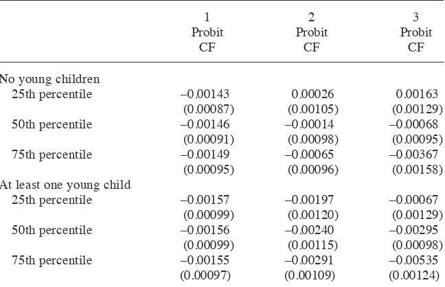
One of the benefi ts of using a nonlinear model is that it allows the effects of the explan-atory variables to change in a parsimonious way. Table 4 provides estimates of average partial effects for nwifeinc, evaluated at the median as well as the fi rst and third quartiles. I also consider the APEs with and without a young child. All of the other variables are averaged out. The picture is now different than that for the simple model; those APEs are reported in Column 1 of the table. When nwifeinc appears linearly in the probit model, its APE is essentially fl at across the six combinations of (kidlt6, nwifeinc). By contrast, in Column 2, the APEs vary substantially across different settings of the two covariates. The effect of nwifeinc is essentially zero at the three income settings for women without a young child although the point estimates show the effect increases in magnitude as income increases. For women with a young child, the effect is marginally signifi cant at the lowest quartile, –0.0020 (t = –1.65), and is largest at the 75th percentile, –0.0029 (t = –2.67).
Finally, Column 6 in Table 3 contains estimated parameters of a model that adds a quadratic in the CF, vˆ
i2, along with an interaction between vˆi2 and nwifeinci. Now the
three terms that depend on the CF are jointly very signifi cant, with p–value equal to zero to four decimal places. Plus, each term is individually very signifi cant, suggesting that the earlier models suffer from functional form misspecifi cation. As often happens in comparing a variety of models, the estimated APE across all observations is very similar to the simpler models, including the linear model estimated by IV: –0.0015 (t = –1.50). But the pattern of APEs at different (kidlt6, nwifeinc) pairs differs. Column 3 in Table 4 contains the APEs. Now nwifecinc has a negative, statistically signifi cant Table 4
Average Partial Effects of nwifeinc at Different Quartiles
1
Notes: (i) Column 1 is for the probit estimates reported in Column 4 of Table 3, Column 2 corresponds to Column 5 in Table 3, and Column 3 corresponds to Column 6 in Table 3.
effect at the highest quartile among women without a small child: –0.0037 (t = –2.32). Among women with a child, there is no income effect at the lowest quartile but a fairly large effect, –0.0054 (t = –4.31), at the highest quartile.
There is no guarantee that even the last model captures all of the important non-linearities, but the example shows that accounting for the nonlinearities is potentially important. With large sample sizes, one can try interactions among all variables—in-cluding the control function—and quadratics in the continuous variables (invariables—in-cluding the control function). Two- step estimation is simple and the bootstrap effi ciently com-putes standard errors of the coeffi cients and the average partial effects.
The BP setup, and therefore convenient parametric approximations, extends easily to the case of a vector of continuous EEVs, say y2, provided there are suffi cient instru-ments. An example is Petrin and Train (2010), which studies multinomial consumer choice models with a vector of endogenous price variables. Rather than start with, say, a multinomial or nested logit model that depends on unobserved taste heterogeneity that can be correlated with price, Petrin and Train proposes estimating such models for
D(y1|z1,y2,v2), where v2 is the vector of reduced for errors in y2= ⌸2z+v2. When v2 is replaced with reduced- form residuals vˆi2—obtained from OLS regressions using prices or log prices—the CF methods are computationally simple even for many choice alternatives. The standard approach, where the distribution of the heterogeneity is modeled and then integrated out, is much more complicated. Petrin and Train pro-vides evidence that the CF approach works well.
B. Discrete EEVs
The major impediment to extending the BP framework to allow discrete EEVs is that the average structural function is nonparametrically unidentifi ed even under fairly strong independence assumptions; see Chesher (2003). Consequently, parametric CF approaches when y2 is discrete generally require the parametric assumptions to hold in order to achieve identifi cation. By contrast, the parametric models discussed in the previous subsection are offered as fl exible approximations to an analysis that, in prin-ciple, could be fully nonparametric.
The traditional approach to estimating nonlinear models with discrete y2 is not a CF approach. Instead, maximum likelihood—or, in some cases, quasi- MLE (see Wooldridge 2014 for some recent examples)—is by far the leading method. One oc-casionally sees plug- in methods used but these are generally inconsistent. In this sub-section, I discuss how two- step CF methods can be used in place of MLE approaches under a different set of parametric assumptions. The CF approach is somewhat contro-versial in this case because the assumptions under which it produces consistent partial effects are nonstandard.
To illustrate the issues, suppose that y1 is binary and is generated by Equation 34. Now, y2 is also binary and follows a linear index model:
(51) y2=1[z␦2+v2≥0].
standard normal. This model is sometimes called a “bivariate probit” model, where y2 appears in the equation for y1 but Equation 51 is taken to be a reduced form probit equation. The ASF, ⌽(z1␦1+␥1y2), is easily estimated given the MLEs of ␦1 and ␥1. A
plug- in approach that replaces yi2 with probit fi tted values, ⌽(zi␦ˆ2), in the second- stage
probit inconsistently estimates both the parameters and the average partial effects. Under the standard bivariate probit assumptions, there is no known CF method that consistently estimates the parameters. Nevertheless, as shown by Wooldridge (2014), an optimal test of the null hypothesis that y2 is exogenous is obtained as the usual MLE t statistic on the generalized residual rˆi2 = yi2(zi␦ˆ2)−(1− yi2)(−zi␦ˆ2). Therefore, if
one knew ␦2, rather than having to estimate it, one would estimate the probit model
(52) P(yi1=1|zi1,yi2,ri2)=⌽(zi1␦1+␥1yi2+1ri2)
and test H0:1=0. To operationalize the test, replace ri2 with rˆi2.
An intriguing possibility is that including rˆi2 in the second- stage probit along with (zi1, yi2) might provide an accurate correction for “small” amounts of endogeneity, where smallness is measured by the size of 1. Terza, Basu, and Rathouz (2008) (TBR) was the fi rst to propose adding residuals to standard models—such as probit—to solve the endogeneity problem for discrete y2. Rather than the generalized residual rˆi2, TBR uses the residual eˆi2= yi2−⌽(zi␦ˆ2), but the motivation is the same. As noted by
Wooldridge (2014), in order to use Equation 52 to consistently estimate the average partial effects, one needs to add the assumption that r2 acts as a kind of suffi cient sta-tistic for capturing the endogeneity of y2. One can state the condition by recalling that
y1=1[z1␦1+␥1y2+u1≥0]. Then, assume that u1 depends on (z, y2) only through r2 in the conditional distribution sense:
(53) D(u1|z,y2)= D(u1|r2).
When Equations 52 and 53 are combined, the average structural function can be con-sistently estimated, just as in the BP case, by averaging out the generalized residuals:
(54) pASF(z1,y2)= N− 1
i=1
N
∑
⌽(z1␦ˆ1+␥ˆ1y2+ˆ1rˆi2).In using Equation 52 as an estimating equation, I still require that zi has at least one element with nonzero coeffi cient in ␦2 that is excluded from zi1. This ensures that ri2 has variation that is not determined entirely by (zi1, yi2). As with any CF method, it is better to have more independent variation in ri2. Because ri2 depends on zi in a nonlin-ear way, technically I could get by with zi = zi1. However, as in other contexts, I should not achieve identifi cation off of nonlinearities. That is, if a linear version of the model is not identifi ed, then I should not proceed with a nonlinear model. For further discus-sion, see Wooldridge (2010, Section 9.5).
It is important to understand that the CF approach and the bivariate probit approach use the same probit reduced form for y2 but use different assumptions about the con-ditional distribution D(y1|z,y2). The bivariate probit approach requires an extra
approximation for 1 “near” zero, the simple CF method might provide good estimates of the ASF fairly generally.
Using the data in AET, but with only 5,979 students due to missing data on the bi-nary response y1 = hsgrad, the probit model in Equation 52 can be estimated by insert-ing the same generalized residuals used for the linear math12 equation. The exogenous variables are exactly as before, with the distance dummies playing the role of instru-ments. The coeffi cient from the second stage probit on rˆi2 is 0.626 (t = 3.15), suggest-ing a strong form of self- selection into attendsuggest-ing a Catholic high school. The average partial effect of cathhs using the two- step CF approach is actually negative, –0.082, with p–value above 0.25. Thus, in this simple model, there is no evidence that attend-ing a Catholic high school has a positive causal effect on graduatattend-ing from high school. When the generalized residuals are dropped so that cathhs is treated as exogenous, the APE is 0.047 (t = 4.92), suggesting a nontrivial positive and very statistically signifi -cant effect. A complete set of estimates is available on request.
As in the case with a continuous EEV, I can use fl exible parametric models to allow general interactive effects inside the probit function. For example,
(55) P(yi1=1|zi,yi2,ri2) = ⌽(xi11+1ri2+xi1ri21),
where x1 is a general function of (z1, y2) and includes an intercept. I can use a standard Wald test of H0:1=0,1=0 after replacing r
i2 with its generalized residuals from the fi rst- stage probit. The average structural function is estimated as in Equation 50 with rˆi2 replacing vˆi2.
If one embraces the fl exibility of the control function approach when combined with sensible parametric functional forms, problems that can be computationally de-manding using traditional approaches become much easier. For example, in the binary response model, there might be a continuous EEV, say y2, and a binary EEV, say y3. One can include functions of the OLS residuals from the reduced form for y2 and the generalized residuals from the reduced form probit model for y3 in a second- stage probit model for y1. These functions might include quadratics, cubics, and various interactions among the OLS residuals, generalized residuals, and observed covariates.
V. Concluding Remarks
This survey of control function methods has focused on cross- sectional applications where the average partial effects on a mean response function are of pri-mary interest—hence my focus on the average structural function. But one need not focus on the mean. For example, Imbens and Newey (2009) defi nes the notion of a “quantile structural function” and derives control function methods under monotonic-ity. It is important to understand that such a change of focus often restricts the amount of heterogeneity that one may have in a model, especially when one approaches the problem from a nonparametric perspective.