The Long-Term Effects of Youth
Unemployment
Thomas A. Mroz
Timothy H. Savage
a b s t r a c t
Using NLSY data, we examine the long-term effects of youth unemployment on later labor market outcomes. Involuntary unemployment may yield sub-optimal investments in human capital in the short run. A theoretical model of dynamic human capital investment predicts a rational “catch-up” response. Using semiparametric techniques to control for the endogeneity of prior behavior, our estimates provide strong evidence of this response. We also find evidence of persistence in unemployment. Combining our semi-parametric estimates with a dynamic approximation to the lifecycle, we find that unemployment experienced as long ago as ten years continues to affect earnings adversely despite the catch-up response.
I.
Introduction
This research jointly models the endogenous schooling, training, and labor market decisions and outcomes of young men over time using a sample from the 1979 National Longitudinal Survey of Youth (NLSY79). We use an econometric
Thomas A. Mroz is a professor of Economics at the University of North Carolina at Chapel Hill and the Carolina Population Center; tom_mroz@unc.edu. Timothy H. Savage is a researcher with the ERS Group, tsavage@ersgroup.com. The authors are grateful to Donna Gilleskie and David Guilkey for their valuable comments on prior drafts. They thank Brian Surette for his FORTRAN code and Alex Cowell for supple-mentary state-level data on schooling expenditures and tuition costs. Tetyana Shvydko provided excellent research assistance. Many useful comments on earlier drafts came from seminars at Duke, UNC, the Stanford Institute for Theoretical Economics, the World Bank, the Federal Reserve Bank of New York, the University of Iowa, and Yale. The authors take responsibility for any remaining errors. The Employment Policy Institute provided partial funding for this research project. The confidential GEOCODE NLSY data used in this article are available to other researchers if they apply to the Bureau of Labor Statistics. The application to obtain the GEOCODE can be obtained at www.bls.gov/nls/geocodeapp.htm. The authors would be happy to provide guidance to another researcher pursuing use of these data.
[Submitted July 2004; accepted August 2005]
ISSN 022-166X E-ISSN 1548-8004 © 2006 by the Board of Regents of the University of Wisconsin System
framework that includes detailed controls for the endogeneity of a wide range of human capital behaviors, including prior unemployment. As a result, we are able to estimate policy-relevant effects of youth unemployment on labor market outcomes later in life.
A spell of unemployment can lead to suboptimal investments in human capital among young people in the short run. A general dynamic model of human capital investment and accumulation predicts a rational “catch-up” response to an involuntary unemployment spell. The estimates presented here provide strong evidence of this catch-up response. We find that recent unemployment has a significant positive effect on whether a young man trains today. While there is little evidence of significant long-lived persistence of unemployment spells on the incidence and duration of future unemployment spells, there is short-term persistence.
Despite this catch-up response and an absence of long-lived persistence in unem-ployment spells, there is evidence of long-lived “blemishes” from unemunem-ployment. Dynamic simulations using an approximation to the lifecycle optimization process indicate that a six-month spell of unemployment experienced at age 22 would result in an 8 percent lower wage rate, on average, at age 23. This wage effect occurs whether we “assign” unemployment to all working individuals in the sample or if we use increases in local unemployment rates to “induce” those most at risk of layoff into unemployment. The former scenario represents a population-average effect, while the latter is a form of a local-average treatment effect. Wages remain more than 5 percent below their undisturbed level through age 26, and even at ages 30 and 31 wages are 2–3 percent lower than they otherwise would have been. In 2002 U.S. dollars at 2,000 hours per year, a six-month spell of unemployment at age 22 yields a $1,400 to $1,650 earnings deficit at age 26 (about 6 percent) and a $1,050 to $1,150 deficit (about 4 per-cent) at age 30, depending on the type of average effect one considers.
II.
Prior Literature
Viewing youth unemployment as involuntary, early empirical analy-ses of the long-term effects of youth unemployment focused on the extent to which early unemployment spells affected the incidence and duration of future spells, as in Stevenson (1978) and Becker and Hills (1980). They predicted dire consequences for those young people who experienced unemployment early in their working lives. Drawing on the human capital models of Ben-Porath (1967) and Blinder and Weiss (1976), other analyses posited that early spells would deprive the young of labor force experience during that portion of the lifecycle when it yields the highest return. As a result, the lifetime earnings profiles of unemployed youths would perma-nently shift down. Such analyses found empirical evidence of strong persistence in unemployment.
In contrast, Heckman (1981), Heckman and Borjas (1980), and Flinn and Heckman (1982, 1983) drew a distinction between true state dependence and unobserved het-erogeneity. Hypothesizing that individuals differ in certain unobserved characteris-tics, these studies demonstrated that a failure to control for heterogeneity might spuriously indicate causal persistence. If such characteristics were correlated over time, measures of state dependence act as proxies for this serial correlation in the absence of suitable controls. Young people with weak preferences for work, for The Journal of Human Resources
instance, will tend to work less over time other things equal. Observed variables such as prior unemployment are, therefore, statistically endogenous in regression analyses and unbiased measures of their effects on future spells cannot be obtained.
A 1982 National Bureau of Economic Research (NBER) volume on the youth labor market approached the subject of youth unemployment, in part, by drawing on the search-theoretic framework of Mortensen (1970) and Lippman and McCall (1976). Many of the analyses in this volume posit that an extensive process of mixing and matching among workers and firms characterizes the youth labor market. Young peo-ple change jobs frequently due to low reservation wages and low opportunity costs. High turnover rates, possibly punctuated by unemployment spells, are a natural char-acteristic of this market and, as such, are not a source of concern. Freeman and Medoff (1982), Freeman and Wise (1982), and Topel and Ward (1992) discuss this interpretation. Within the context of this analysis, three papers of the NBER volume merit discussion.
First, Corcoran (1982) examines persistence in employment status by examining whether current employment status is influenced by prior employment status using data from the National Longitudinal Survey of Young Women. She finds the odds that a young woman works this year are nearly eight times higher if she worked last year than if she did not. Using a sample of young women who have finished school, she also examines the effect of prior education and work experience on hourly earnings and finds that both positively affect wages for the first few years out of school.
Second, Ellwood (1982) examines persistence in employment patterns using annual weeks of unemployment and annual weeks worked using data from the National Longitudinal Survey of Young Men. After controlling for unobserved het-erogeneity with a fixed-effects specification, he finds no persistence in unemployment and slight evidence of persistence in work behavior. He also examines the effect of prior education and work experience on hourly earnings, finding that both have a sig-nificant and positive effect for the first few years out of school. In both the Corcoran and Ellwood studies, the cost of forgone participation appears to be lower future wages rather than persistent nonparticipation in the labor market. If unobserved tastes vary as young people age, neither of these studies controls appropriately for unob-served heterogeneity. Variables such as schooling or prior unemployment remain endogenous, and estimates of their effects on outcomes such as hourly earnings are biased. Furthermore, evidence from Lewis (1986) and Robinson (1989) indicates that the fixed-effects specification exacerbates problems of measurement error in a man-ner that biases estimates toward zero.
Third, using normal maximum likelihood methods to control for endogeneity, Meyer and Wise (1982) model jointly the choices of schooling and annual weeks worked. Separately, they also jointly model the schooling decision and wages. Using data from the National Longitudinal Survey of 1972 High School Seniors, they find that hours of work during high school positively affect weeks worked after graduation and that early labor force experience positively affects wages. While they recognize that schooling, experience, and wages should be modeled and estimated jointly, they only consider bivariate models.
There are several other papers that fit within the context of this research. Michael and Tuma (1984) regress wages on lagged experience and schooling for 14- and 15-year-olds from the NLSY and find that early employment does not affect wages or
schooling likelihood two years later. They treat early experience as exogenous. Using a similar sample, Ghosh (1994) also treats early decision-making as exogenous but uses test scores to proxy for heterogeneity. He finds that early experience has pos-itive effects on hours worked and wage rates at ages 22 and 23. Other relevant research includes Lynch (1985), Lynch (1989), Narendranathan and Elias (1993), Raphael (1996), and the Report on the Youth Labor Force by the US Department of Labor (2000).
In a subsequent NBER volume on the youth labor market, Card and Lemieux (2000) hypothesize that young people adapt to changes in labor market conditions in a variety of ways. Using samples from the U.S. Current Population Survey and the Canadian Census, they find that weaker labor market conditions and lower wages increase the likelihood that young men stay at home with their parents, as well as remain in school. Their hypotheses, however, are not ultimately tied directly to a for-mal model of optimization under uncertainty. Burgess, Propper, Rees, and Shearer (2003), using British data, find that the impact of early career unemployment on later employment outcomes varies according to an individual’s skill level, with the lesser skilled being more prone to suffer adverse consequences later in life.
A number of studies have used displaced workers to examine the consequences of layoffs on subsequent wage rates and earnings. Nearly all of these studies find sub-stantial effects for older individuals, whereas Jacobson, LaLonde, and Sullivan (1993) find that the longer-term adverse effects tend to be smaller for younger workers. In particular, Topel (1990) finds more complete convergence in the wages of younger displaced individuals when compared to their nondisplaced counterparts. In a study of the impacts of displacement on young people, Kletzer and Fairlie (2003) use NLSY79 data and find that the wage gap between displaced and nondisplaced men grows through at least five years after displacement. Their results differ from the results that we report here due largely to the fact that the comparison group they use, as is done in many displaced-worker studies, consists of individuals who never have experienced a spell of unemployment. As Stevens (1997) demonstrates, much of the estimated per-sistence in low earnings after displacement can be attributed to the fact that the dis-placed worker group can experience multiple spells of unemployment. For policy purposes, it may be more reasonable to ask what would happen if one could prevent a single spell of unemployment for a young person rather than asking what would happen if one could forever banish unemployment. Our economic model and empiri-cal analysis examine what would happen if one were able to prevent a single spell of unemployment.
This research contributes to the literature on youth unemployment by directly addressing existing deficiencies such as the lack of a theoretical foundation, the use of small or nonrandom samples, a failure to control adequately for unobserved hetero-geneity and endohetero-geneity, insufficient time horizons to evaluate the full impacts of early unemployment, and the imposition of unnecessarily restrictive statistical assumptions.
III. A Conceptual Framework
Consider the following analytic model of human capital investment. The model is similar to Ben-Porath’s (1967) classic model with the addition of ran-The Journal of Human Resources
dom unemployment shocks that affect one’s ability to earn and train.1In this model, the present and the future are linked through the process of human capital accumu-lation. An exogenous shock that perturbs the optimal time-path of human capital investment in one period persists through time via its effects on additions to the human capital stock. The model is used to examine the effects of this shock on future behaviors and outcomes.
In this model, individuals live with certainty for Tperiods and may train in each of the first T-1 periods. For the moment, assume, as in Ben-Porath, that there is no unem-ployment. At the beginning of period t, an individual’s human capital stock is given by Ht. Individuals invest in additional human capital by devoting a fraction of their time, st, to human capital production, which we call training. Training occurs on the job and is considered to be general. There are no savings, no human capital depreci-ation, and no decisions regarding hours of work other than the choice of the fraction of time to devote to investments and away from current earnings. Potential earnings,
Et*, can be obtained by renting the human capital stock at a constant rate w: Et* = wHt. It is always possible to obtain these earnings, except when experiencing involuntarily unemployment. Disposable income (or net earnings) is the difference between poten-tial earnings and the opportunity cost of human capital used in the production process, or Et= (1 −st)wHt.
At the beginning of each period, an individual chooses the fraction of his time to devote to the production of new human capital, st. Human capital at the start of the next time period is given by Ht+1= Ht+f(st*), where st* is the actual amount of time that ends up being devoted to producing new human capital. In the absence of unem-ployment, st* = st. The human capital production function is assumed to be increasing in its argument and strictly concave.
We assume that all unemployment is involuntary and that individuals have rational expectations about the probability of experiencing unemployment. The probability of unemployment does not depend on the individual’s choice of st. All training and earnings for each time period take place on the single job chosen at the start of the time period (indexed by the value of st) before the individual’s unem-ployment status is revealed. When unemunem-ployment strikes, it reduces disposable earnings and optimally planned training time on the job by equal percentages. In particular, let (1 − λ) be the fraction of the time period that the individual spends unemployed. If he experiences unemployment, then his actual disposable earnings in the time period would be Et = λ(1 − st)wHt, and the additions to the human capital stock during the period he is unemployed would be given by f(λst).2 Unemployment, therefore, perturbs an individual’s optimal time-path of human capital accumulation by preventing on-the-job training. This results in an
underin-Mroz and Savage 263
1. Ben-Porath uses a continuous-time framework, while the model described here is in discrete time. Unlike Ben-Porath, we do not require the human capital production function to exhibit Harrod-neutral technical change. See Supplementary Appendix 1 on the JHR website, www.scc.wisc.edu/jhr/, for a complete presen-tation of the model.
vestment in human capital after the unemployment spell occurs. One can view unemployment at time t, then, as an exogenous reduction in the amount of human capital available at the start of period t+1.
Those who experience an unemployment spell in the preceding period enter the current period with a lower stock of human capital than otherwise identical individu-als. Crucially, having experienced the shock, individuals are able to reoptimize at the start of the next period; this yields a new optimal time-path of human capital invest-ment. Besides lowering lifetime expected wealth, the only lasting effect of an invol-untary unemployment spell is that it constrains an individual to less human capital accumulation than he had planned. This model is used to examine how a spell affects observable outcomes such as earnings and training, and it provides a mechanism through which adverse effects may be mitigated by behavioral responses. It yields three key propositions.
The first proposition states that after experiencing an involuntary unemployment spell in any period before T-1, an individual will unambiguously increase the time that is spent training in the next period. This proposition implies that a young person will exhibit an optimal training “catch-up” response to an involuntary unemployment spell that exogenously reduces his human capital acquisition at time t. The reoptimization that takes the unemployment spell into account, however, implies an unambiguous effect on future behavior: A young person will increase the future share of time that is spent training. We refer to this change in subsequent, optimal investment choices as a “catch-up” response, and it is directly testable in the data.
The second proposition, the convergence of potential earnings, states that the effect of the unemployment spell on potential earnings diminishes over time. This proposi-tion implies that, because of the optimal response to the human capital shock, the compensatory training behavior results in a convergence in the unperturbed and per-turbed human capital stocks. The “catch-up” behavior directly mitigates the unem-ployment spell’s effect on potential earnings over time. This model demonstrates persistence in the sense that the effect of a spell in a single period lasts beyond that period. Optimizing behavior, however, mitigates that effect over time. Because one cannot observe potential earnings, it is not possible to test this proposition directly in the data. It leads to the third proposition, however, which contains observable implications.
The third proposition, the excessive divergence followed by the excessive conver-gence of disposable earnings, states that observed net earnings immediately after experiencing unemployment are lower than would be implied by solely the reduction in the human capital stock. Furthermore, observed earnings grow faster after the first period following an unemployment spell than would be implied by the conver-gence of the human capital stocks. This proposition implies that the observed differ-ences in disposable earnings between those who were and those who were not recently unemployed are larger than would be implied by the differences in their human capital stocks. To see this, holding fixed the share of time that is spent train-ing, the reduction in earnings would reflect exactly the lower stock of human capital. The optimal catch-up response, however, implies that a recently unemployed individ-ual increases the share of time that is spent training. Therefore, he necessarily decreases the share of time spent producing disposable earnings, which results in observed earnings that are lower than would be implied solely by the reduction in the The Journal of Human Resources
human capital stock. In subsequent time periods, because of the catch-up response, the gap in human capital stocks diminishes between those who had and had not experienced unemployment. Differences in the shares of time spent training, therefore, become less pronounced. The later convergence of disposable earnings reflects both the convergence of the human capital stocks as well as the convergence of the human capital investment decisions.
This conceptual model directly links the present and the future through the process of human capital investment and accumulation. By positing equivalence between an involuntary unemployment spell and an exogenously constrained human capital stock, one can examine the effects of such unemployment on future behavior and outcomes. In our empirical analysis, we assume that observed hourly wages are net of human capital training costs. Wage rate differentials reflect both differences in human capital stocks and differences in the amount of time spent in on-the-job training.
IV. The Empirical Specification, Identification,
and the Data
The preceding conceptual model provides a link between prior unem-ployment and future behaviors and outcomes through the human capital accumulation process. In this model, an exogenous unemployment spell results in suboptimal human capital acquisition that directly affects future decisions and outcomes. Empirically, we jointly model the endogenous schooling, training, and labor market decisions and outcomes of young people over time. As in Mroz and Weir (2003), we use an approximation to the optimal decision rules that could be derived from an explicit solution to the true, underlying stochastic dynamic optimization. While the above simple theoretical framework does suggest particular constraints that one potentially could impose in the estimation of the evolution of wages and training through time in response to unemployment shocks, we do not impose these restrictions. Instead, we estimate unconstrained models and examine whether these theoretical implications are evident in the data.
Each year, a young person chooses whether to train, to attend school, and to par-ticipate in the labor market. If participating, he chooses how many hours to work annually. He also may experience unemployment, either voluntary or involuntary, during the year. Hourly earnings as well as schooling, training, and labor force par-ticipation may be affected by the unemployment. As implied by the theoretical model, these decisions and outcomes depend on all the state variables at the start of each time period. We estimate this system of equations using a semiparametric, full-information maximum likelihood method suggested for single equations by Heckman and Singer (1984) and extended to simultaneous equations by Mroz and Guilkey (1992) and Mroz (1999). This discrete factor maximum likelihood (DFML) method allows complex correlation patterns across equations and over time. It explicitly models and controls for the contaminating effects of heterogeneity and endogeneity.
By using this procedure, we are able to control for the endogeneity of a wide range of the youths’ previous decisions and outcomes on their later behaviors and outcomes. For example, we are able to model the effects of endogenous behavioral determinants
including previous unemployment, job changing, schooling, and work experience. Therefore, the estimates reported in this study can be interpreted as the impacts of exogenously induced changes in the endogenous determinants.
A. Derivation of the Likelihood Function
In a study of this type, there are many potentially endogenous human capital variables that are used as explanatory variables. They include the stocks of education and work experience, as well as prior unemployment. In addition, there are potential self-selection issues for the observed working and training outcomes. To account for these potential sources of bias, up to eight behavioral outcomes are jointly modeled every year for each young person in the sample. These outcomes are (log) average hourly earnings (wit), whether or not a young man works (workit), annual hours worked if working (hwit), whether or not a young man is unemployed (unit), annual weeks of unemployment if unemployed (wuit), whether the individual changed jobs (chit), school attendance (asit), and training (trit). We also specify an initial condition equa-tion to control for the endogeneity of each person’s schooling attainment at the start of the panel (isi).
Let εit be a vector with nine elements that contain unobserved determinants of the above outcomes. These unobserved determinants are specified to have an error-component structure such that εit= ρµi+ ηit+uit, where ρis a matrix of factor loads, µiis a vector of unobserved permanent factors, ηitis a vector of unobserved transi-tory factors, and uitis a mean-zero i.i.d. normal error vector. The only substantive restriction this error-components structure places on the distribution of εitis that all correlation across equations in different time periods enters solely through the linear factors µi. Within time periods, the covariance pattern is unrestricted due to the freely estimated relationships among the elements of ηit, though we do impose that the joint distribution does not vary through time. The factors µicapture unobserved determi-nants that do not vary as young people age such as, perhaps, ability. The factor ηit captures time-specific unobserved determinants that may vary across time such as preferences for work. It allows for arbitrary, contemporaneous correlation of out-comes at each point in time that is not captured by the person specific unobserved factor.
As an example of a discrete outcome, consider training, trit. As with the other four dummy variable outcomes modeled in this study, a latent index specification is used.
At each point in time, a young man trains if the value of his latent index is positive. The decision to train is influenced by a vector of observed variables, xtr,it. This vector of variables, listed in Tables 1 and 2, includes background characteristics together with demographic and (potentially endogenous) human capital variables. Crucially, the decision to train is also influenced by prior unemployment and prior job changes for up to five years. Unobserved permanent and transitory factors also influence training. The Journal of Human Resources
As an example of a continuous outcome, consider annual hours worked.3 (2)
x wu +x c ch +t n +h +u
冱
冱
hit xhit h h, it ch, it h i hit hit
5 5
l
= a + b
=1 x -x =1 x -x l
Every year for each young man, annual hours of work are influenced by a vector of observed variables and unobserved factors. As with the other outcomes, hours of work are also influenced by prior unemployment and job changes for up to five years. This study focuses on the estimates of the βs, the impacts of prior unemployment, for each of the eight outcomes: βo,τfor o = as, tr, work, hw, un, wu, ch, w, and τ= 1, . . . , 5.
Mroz and Savage 267
Table 1
Averages of Time-Invariant Characteristics (Standard deviations in parentheses and omitted for dummy variables)
Entire Representative Over
Variable Variable Sample Sample Sample
Name Description N = 3,731 N = 2,286 N = 1,445
afqt Armed forces 0.00 8.14 −12.88
qualification test score (28.13) (28.35) (22.40)
initsch Initial level of 9.64 9.75 9.45
schooling (1.67) (1.63) (1.71)
mohgc Mother’s highest 10.86 11.60 9.68
grade completed (3.12) (2.63) (3.46)
fahgc Father’s highest 10.96 11.90 9.46
grade completed (3.64) (3.38) (3.54)
readmat Age 14: Household 0.81 0.89 0.69
received newspapers or magazines
libcard Age 14: Household 0.68 0.72 0.61
had a library card
prot Age 14: Young man 0.50 0.50 0.49
raised protestant
livpar Age 14: Young man 0.67 0.75 0.55
lived with both parents
black Black in random sample 0.07 0.11
hispanic Hispanic in random sample 0.05 0.07
overblack Oversampled Black 0.24 0.69
overhisp Oversampled Hispanic 0.15 0.31
The Journal of Human Resources
268
Table 2
Averages of Time-Variant Characteristics (Standard deviations in parentheses and omitted for dummy variables)
Variable Variable 1979 1986 1993
Name Description N = 3,731 N = 2,805 N = 2,304
un Any unemployment during the year 0.30 0.29 0.19
wun Annual weeks of unemployment (entire sample) 3.32 4.20 2.83
(8.00) (9.75) (7.97)
work Any work during the year 0.58 0.93 0.93
hw Annual hours worked (entire sample) 627.97 1,814.14 2,026.20
(776.92) (909.24) (904.26)
lnw Log of average hourly earnings from wages and 1.31 1.76 2.02
salary (in 1982 dollors) (0.79) (0.73) (0.66)
anysch Any schooling during the year 0.89 0.20 0.07
train Any training during the year 0.03 0.12 0.18
chjob Change job in prior year 0.0027 0.1027 0.0660
age Age 16.55 23.54 30.52
(1.60) (1.63) (1.63)
exp Cumulative labor force experience in hours/2000 0.24 4.39 11.29
(0.35) (2.55) (4.35)
hgc Highest grade in years completed 9.64 12.51 12.96
Mroz and Sa
v
age
269
geddeg Holds a general equivalence degree 0.01 0.09 0.12
hsdeg Holds a high school diploma 0.15 0.66 0.69
coldeg Holds a four-year college degree 0.00 0.12 0.19
urb Residence is urban 0.80 0.82 0.81
ne Residence is Northeastern United States 0.20 0.18 0.17
nc Residence is North-Central United States 0.26 0.25 0.26
so Residence is Southern United States 0.36 0.37 0.37
we Residence is Western United States 0.19 0.20 0.20
ur Local labor market unemployment rate (in percentages) 6.31 7.77 7.53
(1.97) (2.84) (2.60)
expsec Per-pupil public expenditure on secondary 3,107.27 3,694.57 4,056.55
institutions (in 1982 dollars) (732.91) (930.58) (1,042.62)
expps Per-pupil public expenditure on postsecondary 5,735.19 6,454.09 6,828.19
institutions (in 1982 dollars) (1,122.29) (1,135.09) (1,154.78)
ugtuit Undergraduate tuition at main campus of 1,142.54 1,475.57 2,067.79
state university (in 1982 dollars) (391.76) (540.10) (753.73)
mw The larger of federal or state-level hourly 3.93 3.07 2.97
We control for the contaminating effects of heterogeneity and endogeneity by inte-grating out the unobserved factors, µiand ηit. For example, if the researcher assumed that the factors were normally distributed, he could use multivariate normal maximum likelihood. The DFML method used in this study, however, assumes that the underly-ing continuous distributions of the factors can be suitably approximated by discrete distributions with mass points and probability weights that are estimated jointly with the other parameters in the system. Therefore, the researcher does not have to make a priori assumptions about the distribution of the factors since the discrete approxi-mation is driven by the data.
Conditional upon the unobserved factors, µiand ηit, the contribution to the likeli-hood of individual iin year tis: is the annual weeks unemployed density, and Θ is a vector of parameters to be estimated.
Approximating the continuous distributions of µi and ηit with mass points µ1j,
j= 1, . . . ,J, µ2k, k= 1, . . .K, and vector ηm, m= 1, . . , M, the unconditional contri-bution to the likelihood function of individual iis:
(4)
fis(.) is the density for the endogenous initial condition describing schooling com-pleted at the start of the longitudinal survey, and Γis the vector containing the param-eters of the discrete distributions. Complete specifications for all equations, along with point estimates, standard errors, and a discussion of identification in panel data models of this form, are reported in Supplementary Appendix 2 on the JHRwebsite, The Journal of Human Resources
www.scc.wisc.edu/jhr/. We used FORTRAN programs with analytic first derivatives, in conjunction with the optimizer GQOPT, to obtain the maximum likelihood estimates.
To assess some of the more important findings in this paper, we use single-equation approaches to estimate the impact of prior unemployment on particular outcomes of interest. For continuous dependent variables, these are OLS and fixed-effects regressions. For discrete dependent variables, these are probit and Chamberlain’s conditional/fixed-effect logit. For the most part, these alternative approaches provide estimates that are qualitatively similar to those from the discrete factor maximum likelihood approach, and in only one instance do we find evidence of statistically sig-nificant differences between the fixed-effect estimates and the DFML estimates. Note that for the labor market and schooling outcomes that we examine, there may be potentially serious sample selection biases. In most instances, only the DFML estimator has the potential to control for such selection biases when compared to the single-equation approaches. Because much of our analysis explicitly deals with mod-erately complex patterns of prior outcomes influencing current outcomes through the process of human capital accumulation, one should discount the relevance of the con-ditional/fixed-effect logit estimates presented here. As discussed in Chamberlain (1984), this estimator can exhibit considerable bias when the outcome of interest depends on related prior outcomes.
B. Identification
This study treats training, school attendance, work experience, prior job changes, and unemployment as potentially endogenous variables that evolve as the young men in the sample age. These variables are outcomes as well as determinants of later out-comes. Because we treat residence as exogenous, this analysis contains numerous nondeterministically varying, time-dependent exogenous variables, including local unemployment rates, the real level of minimum wages, an urban residence dummy, region dummy variables, real state-level undergraduate tuition levels, and real per-pupil state expenditures on secondary and postsecondary education. As discussed in Bhargava (1991) and Mroz and Surette (1998), panel-data relationships like those examined here implicitly provide many additional identification conditions than one might infer by simply counting the number of contemporaneous exogenous variables, for example, instruments, excluded from a structural equation. Hansen, Heckman, and Mullen (2004) discuss identification conditions in a somewhat related statistical model.
First consider the case of dynamic linear models examined by Bhargava, in which one is willing to impose stability on the structural parameters over time, as we have done. Bhargava derives the reduced-form equations for a system of dynamic equa-tions and demonstrates that every lag of each “instrumental variable” could have a separate impact on the contemporaneous value of an endogenous explanatory vari-able. The time dimension for the exogenous time-varying instruments, therefore, cre-ates a multiplicity of instruments associated with each exclusion restriction, resulting in significantly more degrees of freedom to control for endogenous determinants. His analysis demonstrates that over-identification in linear dynamic models can be obtained under fairly weak conditions.
Second consider the case of dynamic nonlinear models, as discussed in Mroz and Surette, in which identification exploits the fact that variations in the time ordering of the exogenous variables provides even higher degrees of over-identification than would be obtained in linear models. This is because the impact of any lagged exoge-nous variable on a current endogeexoge-nous explanatory variable, in dynamic nonlinear models of the type used here, depends crucially on the precise forms of the prior time series of all exogenous variables. Implicitly, the impact of any single lagged exoge-nous variable is modified by prior lagged values of all other exogeexoge-nous variables. For example, consider the local unemployment rate, which is exogenous to young people at any point in time. In 1985, variation in this rate has a direct impact on 1985 labor market outcomes. Similarly, variation in 1983 has a direct impact on 1983 outcomes. Because of the timing of decision-making, however, the 1983 rate has no direct impact on 1985 outcomes except through the accumulated stock of human capital as of 1985. As a consequence, the 1983 rate is an instrument for the stock of human cap-ital observed in 1985. Additionally, the impact of the 1983 unemployment rate on the accumulated human capital stocks will depend on such factors as school attendance in 1983 (and in earlier years), and those will depend on exogenous factors like tuition costs for 1983 and earlier years. This implies a multiplicity of exclusion restrictions for each of the lagged exogenous variables; Mroz and Savage (2004) provide a more thorough discussion. As long as subsequent values of the lagged exogenous variables cannot be perfectly forecasted in time-separable nonlinear models, there should be an even greater degree of identification than in linear models.
Finally, identification in this model is also secured through contemporaneous, theoretical exclusion restrictions and functional form. Some of the time-varying exoge-nous variables, such as school tuition, can be assumed to affect the schooling and train-ing decisions and labor supply but have no direct impact on wages other than through the human capital stock. They are, therefore, excluded from the wage equation. And, of course, it is certainly the case that our assumed functional forms for index functions do provide identification beyond that which could be achieved in a fully nonparamet-ric model that incorporated only the dynamic exclusion restnonparamet-rictions discussed above. C. The Data
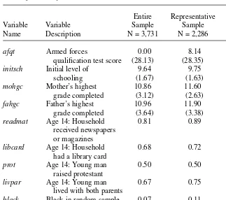
The primary data for this research are taken from the NLSY79 and its GEOCODE supplement. We use young men who were 14 to 19 years old in 1979 from both the representative sample and the oversamples of blacks and Hispanics, yielding a sam-ple size of 3,731, of which 2,286 are from the representative samsam-ple and 1,445 are from the two oversamples. We follow these young men from 1979 through 1994, applying two selection criteria. First, a young man remains in the sample until his first noninterview date, after which he leaves the sample regardless of whether he is inter-viewed at some future date.4Second, those young men not in the initial military sub-sample who enter the armed forces leave the sub-sample permanently upon entry. Table 1 contains variable descriptions and summary statistics for the time-invariant charac-The Journal of Human Resources
272
teristics of our sample. The variable afqt is derived from the 1980 Armed Forces Qualification Test (AFQT). The scores from this test are regressed against age dum-mies to purge pure age effects.5Each value is then mean-differenced using the mean for the entire sample. All monetary variables are measured in 1982 dollars.
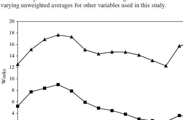
The first eight rows of Table 2 contain the unweighted means for the entire sample in 1979, 1986, and 1993 of the outcomes that are jointly modeled in this study. As shown in Figure 1, average annual weeks of unemployment appear quite anticyclical over this 16-year period, peaking in the recessions of the early 1980s and early 1990s. Figure 1 shows averages both for the entire sample and conditional upon any unem-ployment during the year. School attendance declines monotonically throughout the 16-year period. Participation in vocational training rises to a maximum of 18 percent in 1993 but declines slightly in 1994. Average annual hours of work rise monotoni-cally from 481 in 1979 to 2,034 in 1991. They decline somewhat in 1992 and 1993 but return to their 1991 level by 1994. Real average hourly earnings (in logs) rise monotonically from 1979 to 1993.6The remaining rows in Table 2 contain the time-varying unweighted averages for other variables used in this study.
5. For those in the sample not administered the test, a predicted value is assigned using the race-specific mean residual from the age-adjusted regression.
6. Average hourly earnings are defined as total annual earnings from wages and salary divided by annual hours worked. They are deflated using the CPI-UX1 price index with a base year of 1982. Note that prices approximately doubled from 1982 to 2005.
Mroz and Savage 273
0 2 4 6 8 10 12 14 16 18 20
79 80 81 82 83 84 85 86 87 88 89 90 91 92 93 Year
Weeks
Figure 1
Average Annual Week of Unemployment (Not in School)
Series with triangles is average conditional on any unemployment during the year. Series with diamonds is average for the entire sample
There are several sources of state-level data that we match to the NLSY79 sample. The first comes from the Digest of Education Statistics (DES) on per-student public expenditure at public secondary education institutions. The second is DES data on per-student public expenditure at postsecondary education institutions. The third is data taken from the Integrated Post Secondary Education Data System (IPEDS) on annual tuition prices at the largest or main campus of the state university system. We also match data on mandated minimum wages. Because certain states often have mandates that exceed the federal minimum, we use the larger of the federal or state mandate.
V.
Estimation and Simulation Results
This section discusses the key estimates using the empirical specifica-tion discussed above.7These results are organized into four general topics. The first topic is evidence of a “catch-up” response to unemployment as measured by the effect of an unemployment spell on the probability of training and working and on annual hours worked. The second is evidence of persistence in unemployment. The third is evidence of long-lived “blemishes” of unemployment as measured by forgone average hourly earnings. The fourth section presents simulation evidence of impacts of unemployment on training, later unemployment, work, and wages during the early adult lifetime.
In this section, we compare the DFML estimates to estimates from two types of single-equation specifications mentioned above. According to a likelihood ratio test criterion, the probit/OLS specifications are overwhelmingly rejected in favor of the DFML specification. The log-likelihood value for the independent probit/OLS esti-mates is −230,148.9 based on 364 parameters. The likelihood value for the DFML estimates is −220,859.4 based on 444 parameters. This amounts to an improvement of 9,289.5 in the likelihood value for only 80 additional parameters.
The second type of single-equation specification for comparison uses an individual-specific fixed-effects (FE) model to control for possible unobserved heterogeneity. The FE specification is inconsistent in this setting if, for example, preferences for work fluc-tuate as young people age. In general, we find that the FE point estimates are less precise relative to their DFML counterparts. There is little evidence, however, that the gain in precision with the use of the random-effects DFML specification comes at the expense of consistency. For most key results, such as the wage effect of prior unemployment, the FE point estimates are statistically indistinguishable from DFML estimates.
A. The Catch-Up Response
The conceptual model discussed earlier presents the notion that individuals display an optimal catch-up response to an involuntary unemployment spell. This impetus to
7. A complete set of DFML estimates are in the Supplementary Appendix 2 on the JHR website, www.scc.wisc.edu/jhr/. Our specification uses two permanent linear heterogeneities with five and four mass points respectively and a vector of transitory nonlinear heterogeneities with six mass points. Initial school-ing is modeled only with permanent heterogeneity factors. This specification amounts to 80 additional parameters over a model with no heterogeneity for the 129 possible outcomes we examine for each obser-vation (eight outcomes for each of 16 time periods plus one initial condition).
The Journal of Human Resources
undertake “extra” training mitigates the effect of the spell on potential earnings over time. The DFML estimates strongly support this notion of a catch-up response. Table 3 displays estimates of the effects of prior unemployment on three separate out-comes: whether a young man trains (“Any Training”), whether a young man works (“Any Work”), and how many hours a young man works annually conditional upon working (“Annual Hours Worked”).8
The estimate in the first row of Table 3 indicates that unemployment in the prior period has a significant and positive effect on the likelihood of training in this period. This is the key estimate in this table. To our knowledge, this is the first evidence of such a “catch-up” response in the literature. This training effect, however, is some-what short-lived. The longer-term effects fall to zero quite rapidly. Recent unemploy-ment, after controlling for the endogeneity of the unemployment spell, appears to induce young men to undertake more training.
The other DFML estimates in Table 3 buttress the notion of a compensatory behav-ioral response. There appears to be little response of subsequent work behavior to prior unemployment. Conditional on working, however, the initial effect of prior unemployment on annual hours worked is large and negative, perhaps reflecting the
8. Prior unemployment is measured as weeks per year. The other variables used in these equations are listed in Tables 1 and 2, together with the time period dummies and squares in age and experience.
Mroz and Savage 275
Table 3
Evidence of Catch-Up Response: The Effect of One Week of Unemployment on Training, Work Participation, and Hours Worked
Lag of Annual Weeks of Unemployment
1 2 3 4 5
DFML
Any training 0.0035 0.0011 −0.0019 0.0006 −0.0005
(0.0013) (0.0015) ( 0.0016) (0.0016) (0.0017)
Any work −0.0014 0.0026 0.0087 0.0004 0.0038
(0.0023) (0.0029) (0.0032) (0.0031) (0.0027)
Annual hours −6.1351 1.4876 1.3089 1.3928 1.2408
worked (0.5515) (0.5605) (0.5516) (0.5568) (0.5350)
Fixed effects
Annual hours −8.0821 1.0700 0.5976 1.1307 0.5965
worked (0.5673) (0.5488) (0.5315) (0.5229) (0.5264)
OLSa
Annual hours −11.8621 0.8996 0.6007 1.7038 1.3521
worked (0.6697) (0.6571) (0.6149) (0.5746) (0.5775)
Note: Standard errors in parentheses. a. Robust standard errors.
fact that we assigned weeks of unemployment to the calendar year containing the longest part of a spell interrupted at January 1. Each of the four longer-term effects, however, is significantly positive. A 26-week spell experienced as long ago as five years increases hours worked by 32 hours per year (1.2408 ×26 = 32.26).
Table 3 also presents estimates from FE and OLS estimators for hours worked. Both of these estimators yield point estimates that are more negative for the impact of unemployment experienced last year. The OLS estimates of the former effect indicate a much larger initial negative effect (standard error), −11.86 (0.67), than either of the other two approaches. For additional lags, both alternative estimators tend to indicate smaller responses that vary considerably from lag to lag. The estimates reported in this table support the notion of increased job training immediately after being unem-ployed, as was suggested by the theoretical model. They also suggest increases in hours of work after experiencing unemployment. This effect is not directly captured in our theoretical model, but it is consistent with a spell of unemployment inducing a wealth effect on future hours of work.
The effect of prior unemployment on the probability a young man trains is a key result of this study. Therefore, we compare the DFML point estimates of this effect with two more conventional specifications.9For the DFML specification, the effect of one week of unemployment is equivalent to a 0.41(0.16) percentage-point reduction in the local unemployment rate. Using an identical probit specification (for the explanatory variables), we find the same relative point estimate of 0.41 (0.14). Using a conditional/fixed-effects logit, the effect is equivalent to a 0.32 (0.15) percentage point reduction. Each of these three procedures implies increased training in response to an unemployment spell, and we consider this to be compelling evidence for the catch-up response derived from the theoretical model. Note, however, that neither the probit nor the conditional logit estimators are consistent if past human capital investments are endogenous.
Our specification for training also controls for whether an individual changed jobs during the prior year.10We included this control because it is quite likely that those taking on new jobs might spend some time in formal training programs in order to learn new job skills. If we had failed to control for job changes, an unemployment event might merely be an imperfect signal of a job change and its attendant training. Not one of the three estimation procedures, however, uncovered a significant response of job training to having changed a job in either of the two prior years.
Taken as a whole, the estimates in Table 3, as well as the probit and conditional logit results, provide strong evidence of a catch-up response to unemployment. They indicate that unemployment experienced by a young man today significantly increases
9. These comparisons require a normalization of the different point estimates since they are derived from different probability specifications. For this normalization, we use the estimated coefficient of the local un-employment rate in the training equation because it is an effect that is fairly precisely estimated by each approach. In all instances, higher local unemployment rates appear associated with less training. For the DFML specification, the normalization is 0.00351/(−0.00846) = −0.4149. For probit, it is 0.0035/(−0.0086) =
−0.4070. For conditional logit, it is 0.0062/(−0.01968) = −0.3147. The negative sign indicates that these rel-ative effects can be expressed in terms of a reduction in the local unemployment rate. We treat the denomi-nators as fixed numbers when calculating standard errors.
10. The job change explanatory variables capture both voluntary and unemployment-induced job changes. The Journal of Human Resources
the likelihood of his undertaking training in the near future. The DFML estimates also indicate that unemployment today significantly increases the number of hours he will work (conditional upon working) for up to five years.
B. Persistence in Unemployment
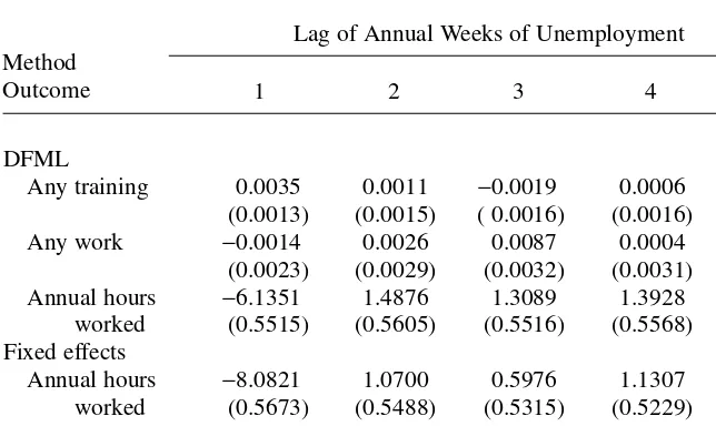
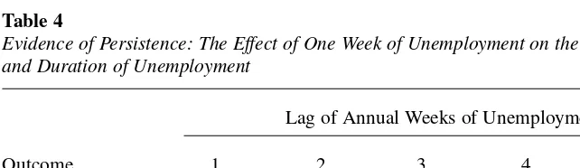
Like many previous studies, we examine how the duration of prior unemployment affects the incidence and duration of future unemployment. In general, the literature shows that controlling for unobserved heterogeneity greatly reduces measured per-sistence in unemployment. The evidence presented here supports that particular find-ing. Many of these previous studies also find that no persistence remains after the use of controls for unobserved heterogeneity. This study disagrees with that finding. We find that there is strong and statistically significant evidence of short-lived persistence in unemployment.
Table 4 displays estimates of the effects of prior unemployment on the probability of experiencing subsequent unemployment and on annual weeks of unemployment if unemployed. The effect for both outcomes is quite pronounced for the first lag, but subsequently diminishes by an order of magnitude or more. Unemployment as long as four years ago, however, has a positive and significant, though quite small, effect on the likelihood of a spell of unemployment.
The positive effect of prior unemployment on the duration of a current spell is short-lived but quite significant. A 26-week spell experienced last year increases the duration of a contemporaneous unemployment spell, if unemployed, by 3.8 weeks annually. The effect is an order of magnitude smaller for all longer lags. Using OLS regressions of current unemployment on prior unemployment, Ellwood (1982) finds strong evidence of state dependence in weeks of unemployment. He finds that all evidence of state dependence vanishes, however, upon controlling for unobserved heterogeneity with FE specifications.
In this study, the OLS and FE estimates for the first lag are qualitatively similar to those in Ellwood’s study: 0.2393 (0.0158) and 0.0073 (0.0157) respectively per week unemployed in the prior year. The OLS estimate indicates a strong influence on later
Mroz and Savage 277
Table 4
Evidence of Persistence: The Effect of One Week of Unemployment on the Incidence and Duration of Unemployment
Lag of Annual Weeks of Unemployment
Outcome 1 2 3 4 5
Any 0.0927 0.0041 0.0068 0.0085 0.0030
unemployment (0.0039) (0.0028) (0.0027) (0.0028) (0.0025)
Annual weeks 0.1447 0.0253 0.0303 0.00138 0.0233
of unemployment (0.0143) (0.0152) (0.0157) (0.0158) (0.0160)
unemployment durations, while the use of a FE specification eliminates all evidence of persistence. On the other hand, the DFML estimate rules out an absence of per-sistence. A specification test of any difference between the FE and DFML estimates rejects the null hypothesis of no difference. This is the only important instance where a DFML estimate appears substantively and statistically different from an associated FE estimate. The FE estimator, however, cannot control well for labor force selection effects and possible schooling selection bias, which could be important early in life.
C. Long-Lived Blemishes
One of the most important measures of the long-term impact of youth unemployment is the effect of a spell on future earnings. Forgone work experience may reverberate throughout a young person’s life. Perhaps this is because one job leapfrogs into another, and early unemployment would delay some of the first jumps. It also may be because lost experience, as posited by dual labor market theorists, permanently tracks young people into jobs characterized by low wages and little room for advancement, as in Topel and Ward (1992) and Cain (1976). Ellwood (1982), for example, finds that prior work experience has a large and positive earnings effect. Forgone experience, therefore, represents lost earnings power. This simple observation is, in fact, the moti-vation for the theoretical model discussed earlier.
Table 5 displays DFML estimates of the effects of prior unemployment on log aver-age hourly earnings. This earnings equation, as with the others in this study, controls extensively for the observed human capital stock. Even with these controls, there is evidence that the direct impact of prior unemployment on earnings is rather more long-lived than most previous studies have shown.
The initial earnings effect of unemployment is large and quite precisely estimated. The DFML estimates tend to be slightly smaller than those derived from FE or OLS specifications, so we focus on them. A 26-week unemployment spell experienced last The Journal of Human Resources
278
Table 5
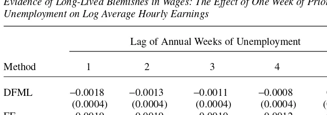
Evidence of Long-Lived Blemishes in Wages: The Effect of One Week of Prior Unemployment on Log Average Hourly Earnings
Lag of Annual Weeks of Unemployment
Method 1 2 3 4 5
DFML −0.0018 −0.0013 −0.0011 −0.0008 0.0002
(0.0004) (0.0004) (0.0004) (0.0004) (0.0004)
FE −0.0019 −0.0019 −0.0010 −0.0012 −0.0000
(0.0006) (0.0006) (0.0005) (0.0005) (0.0005)
OLSa −0.0023 −0.0019 −0.0014 −0.0006 0.0001
(0.0008) (0.0008) (0.0007) (0.0006) (0.0007)
year reduces wages by 4.7 percent. In terms of 2,000 hours worked at the average wage rate in 1993, this is a reduction of over $1,500 in 2002 U.S. dollars.11A two-standard-error lower bound amounts to a 2.6 percent reduction in hourly earnings or over $850. Further, a 26-week spell experienced as long ago as three years reduces wages by 2.9 percent. To put this magnitude into context, this reduction in wages due to experiencing a 26 weeks of unemployment is equivalent to the wage loss from for-going one-quarter to one-half of a year of school.12As predicted by the theoretical model, the earnings effect of prior unemployment tapers off over time. Because it fully dissipates after about four years, the direct impact of unemployment on earnings is not permanent, as suggested by the scar analogy. It is, however, much more than a simple blemish. Unemployment experienced by a young man today will depress his earnings for several years to come.
It is important to note that the negative earnings effect of prior unemployment remains even after extensive controls for the observed and potentially endogenous human capital stock. At first glance, this effect suggests that unemployment does not simply represent forgone human capital, as suggested by dual labor market theorists. There are, however, alternative interpretations for the magnitude and duration of these effects on earnings. First, the human capital variables used in this study are imperfect measures of young men’s human capital stock. The “residual” earnings effect of unemployment that we find could be capturing these imperfectly measured human capital variables. Second, the wage reductions could be reflecting relative increases in on-the-job training for those who recently experienced unemployment.
D. Simulating Unemployment’s Total Impact on Human Capital, Training, and Earnings
The above analysis of the earnings effect of prior unemployment tells only a partial story. A complete story would account simultaneously for the effects of reduced human capital on earnings, as implied by the theoretical model. A complete evalua-tion of the impacts of unemployment must take into account the various avenues through which it can affect later labor market outcomes. Because we model the entire early lifecycle of schooling, training, work, and unemployment, the DFML estimator provides a rich framework to trace out the impacts of unemployment. In this section, we use dynamic simulations with the DFML estimates to undertake such an analysis. These dynamic simulation results measure the total effects of prior outcomes on sub-sequent events, as compared to the partial effects described above.
The literature on local average treatment effects, in particular Angrist, Imbens, and Rubin (1996), highlights the fact that if individuals differ in their responses to a stim-ulus, there are typically an unlimited number of possible average effects that one could evaluate given continuous instrumental (or forcing) variables. In this study, we focus on two of these measures, the population-average effect and one type of the local-average treatment effect. We define the population-average effect as the
11. The average real wage rate in 1993 is $16.42 per hour in 2002 dollars. At 2,000 hours, this yields aver-age earnings of $32,840.
12. The impact (standard error) of an additional year of school on log wages is 0.0791 (0.0209) in the DFML model.
average impact on an outcome of interest if a worker were forced to experience a six-month spell of unemployment at age 22.13In practice, we start with all individuals in our sample who were 14 to 16 years old in 1979, and we simulate outcomes for them to age 21 using the complete set of DFML estimates. For each “individual” at age 22 who was not simulated to be in school or out of the labor force, we then “force” them to experience no unemployment at that age and complete their simulated lifecycle for 10 additional years. We do this 50 times for each individual and use this as a baseline simulation for individuals who were “forced” not to experience unemployment. Next, starting at age 22, we force the same group of individuals to experience 26 weeks of unemployment, a 50 percent reduction in their labor market experience for that year, and a job change. Again, we complete the simulated lifecycle for up to 10 additional years for this group. Our population-average effect, therefore, corresponds to those workers who, at age 22, were forced to experience 26 weeks of unemployment. We refer to this as “Forced Unemployment” in the figures discussed below.
We also consider one form of the local-average treatment effect. To do this, we again examine each of the above “individuals” at age 22. At that age, we ask, for indi-viduals who were not in school and were working but did not experience any unem-ployment, whether an increase of two standard deviations in the local unemployment rate, about five percentage points, would induce them into unemployment. This defines a select group of individuals who, because of their particular configurations of explanatory variables and permanent and transitory heterogeneity at age 22, were sus-ceptible to becoming unemployed when labor market conditions worsen. After iden-tifying this group of individuals, we force them, as above, to experience 26 weeks of unemployment, a 50 percent reduction in their labor market experience for that year, and a job change. Therefore, each individual’s local-average treatment effect is iden-tical to their effect in the calculation of the population-average effect. In fact, the only difference between these two methods of measuring the effects of unemployment is the set of individuals used to define the “average” impact. The local-average effect captures the effect of unemployment on those most likely to be adversely impacted by worsening labor market conditions. We refer to this effect as “Induced Unemployment” in the figures discussed below.
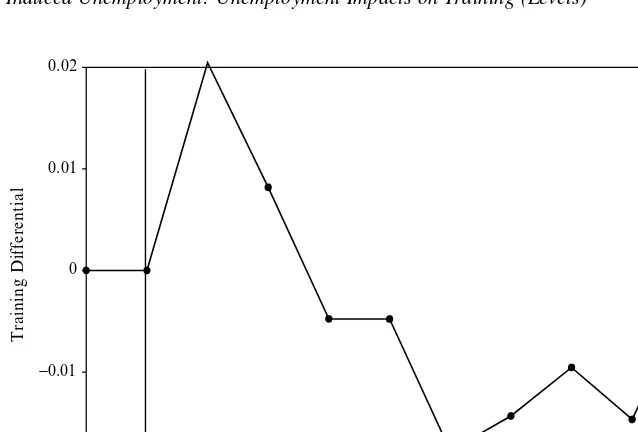
Figures 2a through 2d display simulation results for the impact of forced and induced unemployment at age 22, described above, on job training behavior through age 31. Figures 2a and 2b display information on the population-average effect, while Figures 2c and 2d display information on the local-average treatment effect. In addi-tion, Figures 2a and 2c display the level of training at each age for each treatment effect, while Figures 2b and 2d display the differential in the fraction of training at each age in response to the unemployment event. The series with diamonds on the level figures, 2a and 2c, are for those who experienced unemployment at age 22. All subsequent figures follow the same format as Figures 2a through 2d.
13. We do not use data from the “poor” white subsample because of the peculiar selection issues that might arise. Appropriate weights for aggregating the stratified random samples of the NLSY, however, are not available. Consequently, we do not adjust our estimates to reflect the distribution of teenagers in 1979. The major consequence of this is that our sample overrepresents blacks and Hispanics. The empirical model, however, includes dummies for race and ethnicity.
The Journal of Human Resources
Mroz and Savage 281
0.075 0.1 0.125 0.15 0.175 0.2
21 22 23 24 25 26 27 28 29 30 31 Age
Incidence
Not Unemployed Unemployed
Figure 2a
Forced Unemployment: Unemployment Impacts on Training (Levels)
−0.02 −0.01
0 0.01 0.02
21 22 23 24 25 26 27 28 29 30 31 Age
Training Differential
Figure 2b
The Journal of Human Resources
282
0.075 0.1 0.125 0.15 0.175 0.2
Incidence
Not Unemployed
Unemployed
21 22 23 24 25 26 27 28 29 30 31 Age
Figure 2c
Induced Unemployment: Unemployment Impacts on Training (Levels)
−0.02 −0.01
0 0.01 0.02
Training Differential
21 22 23 24 25 26 27 28 29 30 31 Age
Figure 2d
In the first two years after experiencing unemployment, there is a one- to two-percentage point increase in the incidence of training (about a 10 to 20 percent increase) for both unemployment effects. This is precisely the type of catch-up response suggested by the theoretical model. At age 25 and older, however, there is a slightly lower tendency to train for those who experienced unemployment at age 22. While not displayed here, examination of the simulation results for school attendance indicates a one- to three-percentage point reduction in school attendance rates in the mid-twenties among those who experienced unemployment at age 22. By age 30 there are no appreciable differences in school attendance rates for either type of unemploy-ment effect.
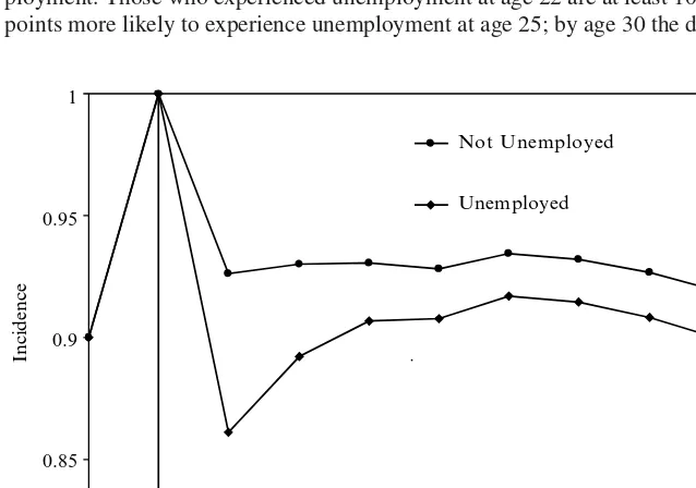
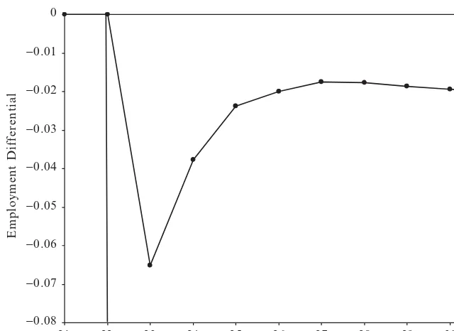
Figures 3a through 3d display simulation results for the impact of forced and induced unemployment at age 22 on employment rates through age 31. For both types of treatment effects, there is evidence of long-lived persistence in the effect of unem-ployment. From ages 25 to 31, employment rates for those who experienced unemployment at age 22 are about two percentage points below the baseline rate. There is some evidence that this persistence is shorter for those who were most likely to be affected by worsening labor market conditions. While not presented here, an examination of the simulated hours of work (conditional on working) indicates a 75-hour-per-year reduction in hours of work for those experiencing unemployment with slightly smaller impacts for the local average treatment.
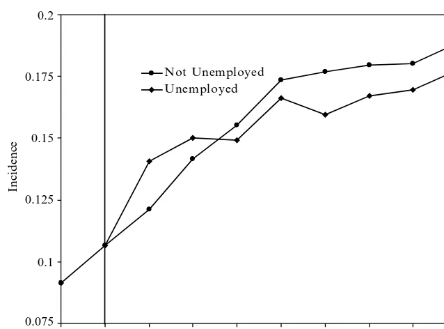
Figures 4a through 4d display simulation results for “state dependence” in unem-ployment. Those who experienced unemployment at age 22 are at least 10 percentage points more likely to experience unemployment at age 25; by age 30 the difference in
Mroz and Savage 283
0.8 0.85 0.9 0.95 1
Incidence
Not Unemployed
Unemployed
21 22 23 24 25 26 27 28 29 30 31 Age
Figure 3a
The Journal of Human Resources
284
−0.08 −0.07 −0.06 −0.05 −0.04 −0.03 −0.02 −0.01 0
Employment Differential
21 22 23 24 25 26 27 28 29 30 31 Age
Figure 3b
Forced Unemployment: Unemployment Impacts on Employment (Differential)
0.8 0.85 0.9 0.95 1
21 22 23 24 25 26 27 28 29 30 31
Incidence
Age
Not Unemployed Unemployed
Figure 3c
Mroz and Savage 285
−0.08 −0.07 −0.06 −0.05 −0.04 −0.03 −0.02 −0.01
0
Age
Employment Differential
21 22 23 24 25 26 27 28 29 30 31
Figure 3d
Induced Unemployment: Unemployment Impacts on Employment (Differential)
0 0.25 0.5 0.75 1
Incidence
Not Unemployed Unemployed
Age
21 22 23 24 25 26 27 28 29 30 31
Figure 4a
The Journal of Human Resources
286
0 0.1 0.2 0.3 0.4 0.5 0.6 0.7 0.8 0.9 1
21 22 23 24 25 26 27 28 29 30 31 Age
Unemployment Differential
Figure 4b
Forced Unemployment: Unemployment Impacts on Subsequent Unemployment (Differential)
1
0.9
0.8
0.7
0.6
0.5
Incidence
0.4
0.3
0.2
0.1
0
21 22 23 24 25 26 Age
Not unemployed Unemployed
27 28 29 30 31
Figure 4c
unemployment rates becomes small. The simulated duration of unemployment effects reveal about one to two additional weeks per unemployed person year at age 23 for those who experienced unemployment at age 22. It falls to essentially zero from age 24 to age 31.
Figures 5a through 5d display simulation results for the impact of forced and induced unemployment at age 22 on the log of average hourly earnings through age 31. After experiencing unemployment at age 22, wages at age 23 are 8–9 percent below their baseline level. According to the theoretical model, an immediate, and excessive, decline in wages would be expected if individuals chose jobs with high levels of on-the-job training after experiencing unemployment. Immediately after age 23, however, the wage differential begins to shrink. The simple theoretical model also predicted this effect. By age 27, the wage difference due to forced or induced unemployment falls to about half its size at age 23. Nevertheless, wages for those young men who experienced forced or induced unemployment at age 22 is still 3–4 percent lower by age 31. Unlike the somewhat relatively short-lived effects implied by the (partial-derivative) point estimates, these simulation results indicate fairly long-lived impacts of unemployment arising through the cumulative impacts on the measured stock of human capital.
The simulation results presented here are generally consistent with the predictions of the theoretical model. There is evidence of increased job training after experienc-ing unemployment. Furthermore, wages appear to fall precipitously in the first year after experiencing unemployment, which could reflect a combination of a relative loss
Mroz and Savage 287
0 0.1 0.2 0.3 0.4 0.5 0.6 0.7 0.8 0.9 1
21 22 23 24 25 26 27 28 29 30 31 Age
Unemployment Differential
Figure 4d
The Journal of Human Resources
288
1.4 1.5 1.6 1.7 1.8 1.9
21 22 23 24 25 26 27 28 29 30 31 Age
Log 1982 Dollars Per Year
Not Unemployed Unemployed
Figure 5a
Forced Unemployment: Unemployment Impacts on Log Wages (Levels)
−0.1 −0.08 −0.06 −0.04 −0.02
0
21 22 23 24 25 26 27 28 29 30 31 Age
Wage Differential
Figure 5b
Mroz and Savage 289
1.4 1.5 1.6 1.7 1.8 1.9
21 22 23 24 25 26 27 28 29 30 31
Age
Log 1982 Dollars Per Hour
Not Unemployed
Unemployed
Figure 5c
Induced Unemployment: Unemployment Impacts on Log Wages (Levels)
−0.1 −0.09 −0.08 −0.07 −0.06 −0.05 −0.04 −0.03 −0.02 −0.01
0
21 22 23 24 25 26 27 28 29 30 31 Age
Wage Differential
Figure 5d