NONLINEAR PROGRAMMING AND ENGINEERING APPLICATIONS

NONLINEAR PROGRAMMING AND ENGINEERING

APPLICATIONS

Robert J. Vanderbei

Princeton University Princeton NJ 08544

rvdb@princeton.edu

Abstract The last decade has seen dramatic strides in ones ability to solve nonlinear pro-gramming problems. In this chapter, we review a few applications of nonlinear programming to interesting, and in some cases important, engineering problems.

Keywords: Sample, edited book

Introduction

Modern interior-point methods for nonlinear programming have their roots in linear programming and most of this algorithmic work comes from the opera-tions research community which is largely associated with solving the complex problems that arise in the business world. However, engineers and scientists also need to solve nonlinear optimization problems. While it is true that many engineers are well aware of the activities of SIAM and therefore are at least somewhat familiar with the advances that have taken place in optimization in the past two decades, there are many engineers and scientists who think that the only tool for solving an optimization problem is to code up something for MATLAB to solve using a genetic algorithm. Often the results are extraordi-narily slow in coming and sometimes not even the results that one was looking for.

developed a desire to see the other side, the user’s side. I became quite interested in applications not just as little toys to illustrate the power of my pet algorithms but rather as important problems that require solution and for which some of my tools might be useful. In this chapter I will chronicle some of these appli-cations and illustrate how modern interior-point methods can be very useful to scientists and engineers.

The next section provides a brief description of an interior-point algorithms for nonlinear programming. Then, in subsequent sections we will discuss the following four application areas:

Finite Impulse Response (FIR) filter design

Telescope design—optics

Telescope design—truss structure

Stable orbits for then-body problem

1.

LOQO: An Interior-Point Code for NLP

Operations Research, our field of study, got its start more than 50 years ago roughly when George Dantzig invented the simplex method for solving linear programming problems. The simplex method together with the development of the computer provided a new extremely powerful tool for solving complex decision making problems. Even today, the simplex method is an indispensable tool to the operations researcher.

Of course, it was fairly soon after the invention that people began to real-ize that the linear programming problem was too restrictive for most of the real-world problems that needed to be solved. Many problems have the extra constraint that some or all of the variables need to be integer valued. Thus was born the field of integer programming. Even more problems involve nonlin-ear functions in the objective function and/or in the constraints and so there also arose the subject of nonlinear programming. The simplex method has played a critical role in both of these directions of generalization. For integer programming, the simplex method is used as a core engine in cutting-plane, branch-and-bound, and branch-and-cut algorithms. Some of these algorithms have proved to be very effective at solving some amazingly difficult integer pro-gramming problems. For nonlinear propro-gramming, the ideas behind the simplex method, namely the idea of active and inactive variables, were extended to this broader class of problems. For many years, the software package called mi-nos, which implemented these ideas, was the best and most-used software for solving constrained nonlinear optimization problems. Its descendent,snopt, remains a very important tool even today.

algorithm has polynomial time worst-case complexity—something that has not yet been established for any variant of the simplex method. Furthermore, he claimed that the algorithm would also be very good in its average-case per-formance and that it would compete with, perhaps even replace, the simplex method as the method of choice for linear programming. True enough, this new class of algorithms, which we now callinterior-point methods, did prove to be competitive. But, the new algorithm did not uniformly dominate the old simplex method and even today the simplex method, as embodied by the com-mercial software package called cplex, remains the most-used method for solving linear programming problems. Furthermore, interior-point methods have not proved to be effective for solving integer programming problems. The tricks that allow one to use the simplex method to solve integer programming problems depends critically on being able to solve large numbers of similar linear programming problems very quickly. The simplex method has the nice feature that solving a second instance of a problem starting from the solution to a first instance is often orders of magnitude faster than simply solving the second instance from scratch. There is no analogous property for interior-point methods and so today the simplex method remains the best method for solving integer programming problems.

So, do interior-point methods have a natural extension to nonlinear program-ming and, if so, how do they compare to the natural extension of the simplex method to such problem? Here, the answers are much more satisfactory. The answer is: yes, there is a very natural extension and, yes, the methods per-form very well in this context. In fact, interior-point methods are really best understood as methods for constrained convex nonlinear optimization.

I have for many years been one of the principle developers of a particular piece of software, calledloqo, which implements an interior-point algorithm for nonlinear programming. In the remainder of this section, I will give a brief review of the algorithm as implemented in this piece of software. The basic family of problems that we wish to solve are given by

minimize f(x)

subject to b_≤h(x)_≤b+r, l≤x≤u,

whereb, h, andr take values inRm _{andl,x, andu take values in}Rm_{. We} assume that the functionsf(x)andh(x)must be twice differentiable (at least at points of evaluation) but not necessarily convex or concave.

The standardinterior-point paradigmcan be described as follows:

Replace nonnegativities with logarithmic barrier terms in objective; that is, terms of the form₋µlog(s)whereµis a positivebarrier parameter andsis a slack variable.

Write first-order optimality conditions for the (equality constrained) bar-rier problem.

Rewrite the optimality conditions in primal-dual symmetric form (this is the only step that requires linear programming for its intuition).

Use Newton’s method to derive search directions. Here is the resulting linear system of equations:

−H(x, y)₋D AT(x)

A(x) E

∆x

∆y

=

∇f(x)−AT(x)y

−h(x) +µY−1_e

.

MatricesDandEare diagonal matrices involving slack variables,

H(x, y) =∇2f(x)−

m X

i=1

yi∇2hi(x) +λI, andA(x) =∇h(x),

whereλis chosen to ensure appropriate descent properties.

Compute a step length that ensures positivity of slack variables.

Shorten steps further to ensure a reduction in either infeasibility or in the barrier function.

Step to new point and repeat.

Further details about the algorithm can be found in LMS94; Van97d.

2.

Digital Audio Filters

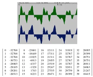
A digital audio signal is a stream of integers, which represents a discretization both in time and in amplitude of an analog signal. For CD-quality sound, there are 44,100 samples per second each sample being a short integer (i.e., an integer between₋32,768and +32,767). Of course, for stereo there are two such streams of integers. Figure 7.1 shows an example of a very short stretch of music.

0 -32768

Figure 7.1. A stereo audio signal digitized.

different speakers. Speakers designed for low frequencies are calledwoofers, those for a middle range of frequencies are calledmidranges, and those for high frequencies are calledtweeters.

Traditionally, the three speakers—woofer, midrange, and tweeter—were housed in the same physical box and the amplified signal was split into three parts using analog filtering components built into the speaker. However, there are limitations to this design. First of all, it is easy to determine the direction of a high frequency signal but not a low frequency one. Hence, the placement of the tweeters is important but the woofer can be put anywhere within hearing range. Furthermore, for stereo systems it is not even necessary to have two woofers—the low frequency signal can be combined into one. Also, woofers are physically large whereas tweeters can be made very small. Hence in a home theater system, one puts small tweeters in appropriate locations on either side of a video screen but puts a single woofer somewhere out of the way, such as under a coffee table.

Hence, using a hefty amplifier on the high frequency component of a signal is wasteful.

Finally, given that the signal is to be split before being amplified it is now possible to consider splitting it even before converting it from digital to analog. At the digital level one has much more control over how the split is accomplished than can be achieved with an analog signal. The most common type of digital filter is a finite impulse response filter, which we describe next.

Finite Impulse Response (FIR) Filters

Afinite impulse response (FIR) filteris given by a finite sequence of real (or complex) numbersh−n, . . . , h−1, h0, h1, . . . , hn. This sequence transforms an

input signal,xk, k ∈ Z, into an output signal, yk, k ∈ Z, according to the

following convolution formula:

yk= n X

i=−n

hixk−i, k∈Z.

Since the sequence of filter coefficients is finite, the sum is finite too. Typically

nis a small number (less than 100) and so the output signal at any given point in time depends on the values of the input signal in a very narrow temporal range symmetric around this time. With 44,100 samples per second,n= 100

corresponds to a time interval that is only a small fraction of a second long. To implement the filter there must be at least this much delay between the input and output signals. Since this delay is small, it is generally unnoticeable.

Of course the filter coefficientshi must be determined when the system is

designed, which is long before any specific input signal is decided upon. Hence, one treats the input signal as a random process which will only be realized in the future but whose statistical properties can be used to design the filter. To this end, we assume thatxkis a stationary second-order random process. This

means that eachxkis random, has mean zero, finite variance, and a covariance

structure that is temporally homogeneous. This last property means that the following covariances depend on the difference between the sample times but not on the time itself:

sk=Exix¯i+k.

(The bar on thexi+kdenotes complex conjugate—most of our processes are

real-valued in which case conjugation will plays no role.) The sequencesk

characterizes the input signal and its Fourier transform

S(ν) =X k

ske2πjkν

taken to be[−1/2,1/2). Valuesν ∈[−1/2,1/2)are calledfrequencies. They can be converted to the usual scale of cycles-per-second (Hz) using the sample rate but for our purposes we will take them as numbers in[−1/2,1/2).

An Example. Consider the simplest input process—a complex signal which is a pure wave with known frequencyν0and an unknown phase shift:

xk=e2πj(k+θ)ν0.

Here,θ is a random variable uniformly distributed on[₋1/2,1/2). For this process, the autocorrelation function is easy to compute:

sk=Exix¯i+k=Ee2πj(i+θ)ν0e−2πj(i+k+θ)ν0 =e−2πjkν0.

The spectral density is given by

S(ν) =

∞ ν =ν0

0 else.

The Transfer Function. We are interested in the spectral properties of the output process. Hence, we introduce the autocorrelation function foryk

rk =Eyiy¯i+k

and its associated spectral density function

R(ν) =X k

rke2πjkν.

Substituting the definition of the output process yi into the formula for the

autocorrelation function, it is easy to check that

rk= X

l

glsk−l,

where

gk= X

i

hihi+k.

Similarly, it is easy to relate the output spectral densityR(ν)to the input spectral densityS(ν):

R(ν) =G(ν)S(ν), (7.1)

where

G(ν) =X k

gke2πjkν.

Linear Phase Filters. For simplicity, we assume that the filter coefficients are real and symmetric about zero: h−i =hi. Such a filter is said to belinear

phase. From these properties it follows that the functionH()defined by

H(ν) =

and the transfer equation can be written in terms ofH():

R(ν) =H(ν)2S(ν).

Power. For stationary signals, the power is defined as the expected value of the square of the signal at any moment in time. So, the input power is

Pin =E|u0|2 =s0=

Z 1/2 −1/2

S(ν)dν

and the output power is

Pout =E|y0|2=r0 =

A signal that is uniformly distributed over low frequencies, say from₋ato

ahas a spectral density given by

S(ν) = 1_[−a,a](ν).

For such a signal, the input and output powers are given by

where

sinc(x) =

sinx

x x6= 0

1 else.

Passbands. In some cases, it is desirable to have the output be as similar as possible to the input. That is, we wish the difference process,

zk=yk−xk,

to have as little energy as possible. Letqkdenote the autocorrelation function

of the difference process:

qk=Eziz¯i+k

and letQ()denote the corresponding spectral density function. It is then easy to check from the definitions that

Q(ν) = (H(ν)₋1)2S(ν).

The output power for the difference process is then given by

Pdiff out =

Z 1/2 −1/2

(H(ν)₋1)2S(ν)dν.

As before, if the input spectral densityS()is a piecewise constant even function, then this output power can be expressed in terms of the sinc function.

Coordinated Woofer–Midrange–Tweeter Filtering

Having covered the basics of FIR filters, we return now to the problem of designing an audio system based on three filters: woofer, midrange, and tweeter. There are four power measurements that we want to be small: for each filter we want the output to be small if the input is uniformly distributed over a range of frequenciesoutsideof the desired frequency range and finally when added together the difference between the summed signal and the original signal should be small over the entire input spectrum. Let

T = (₋1/2,₋bt)∪(bt,1/2),

M = (₋bm,−am)∪(am, bm),

W = (₋aw, aw)

denote the design frequency ranges for the tweeter, midrange, and woofer, re-spectively. Of course, we assume that the three ranges cover the entire available spectrum:

(or, in other words, thatam < awandbt< bm). Each speaker has its own filter

which is defined by its filter coefficients

h(_kj), k=−n,−n+ 1, . . . , n−1, n, j∈ {t, m, w}

and associated spectral density functionHj(ν), j ∈ {t, m, w}.The three

con-straints which say that for each filter the output power per unit of input power is smaller than some thresholdρcan now be written as

1

|Tc_| Z

Tc

H_t2(ν)dν ≤ ρ,

1

|Mc_| Z

Mc

H_m2(ν)dν _≤ ρ,

1

|Wc_| Z

Wc

H_w2(ν)dν ≤ ρ.

It is interesting to note that according to (7.3) the above integrals can all be efficiently expressed in terms of sums of products of pairs of filter coefficients in which the constants involve sinc functions. Such expressions are nonlinear. The fact that these functions are convex is only revealed by noting their equality with the expression in (7.2). Finally, the constraint that the reconstructed sum of the three signals deviates as little as possible from the a uniform response can be written as

Z 1₂

−1 2

(Ht(ν) +Hm(ν) +Hw(ν)−1)2dν≤ǫ.

At this juncture, there are several ways to formulate an optimization problem. We could fixǫto some small positive value and then minimizeρ, or we could fix ρ to some small positive value and minimize ǫ, or we could specify to proportional relation, such as equality, between ρ and ǫ and minimize both simultaneously. To be specific, for this tutorial, we choose the third approach. In this paper (and in life), we formulate our optimization problems inampl, which is a small programming language designed for the efficient expression of optimization problems FGK93. Theamplmodel for this problem is shown in Figure 7.2. The three filters and their spectral response curves are shown in Figure 7.3.

For more information on FIR filter design, see for example WBV97; CS99; LVBL98; Col98.

3.

Shape Optimization (Telescope Design)

function sinc;

param n := 23; param pi := 4*atan(1);

param aw := 0.05; param am := 0.04; param bm := 0.25; param bt := 0.2;

var rho >= 0; var hw {0..n}; var hm {0..n}; var ht {0..n};

minimize power_bnd: rho;

subject to passband:

((hw[0]+hm[0]+ht[0]-1)^2 + 2*sum {k in 1..n} (hw[k]+hm[k]+ht[k])^2) <= rho;

subject to wooferband:

sum {k in -n..n} hw[abs(k)]^2

-sum {k in -n..n, kk in -n..n} 2*aw*hw[abs(k)]*hw[abs(kk)] * sinc(2*pi*(k-kk)*aw) <= (1-2*aw)*rho;

subject to midrangeband: sum {k in -n..n} hm[abs(k)]^2

-sum {k in -n..n, kk in -n..n} 2*bm*hm[abs(k)]*hm[abs(kk)] * sinc(2*pi*(k-kk)*bm) +

sum {k in -n..n, kk in -n..n}

2*am*hm[abs(k)]*hm[abs(kk)] * sinc(2*pi*(k-kk)*am) <= (1-2*(bm-am))*rho;

subject to tweeterband:

sum {k in -n..n, kk in -n..n} 2*bt*ht[abs(k)]*ht[abs(kk)] * sinc(2*pi*(k-kk)*bt) <= 2*bt*rho;

solve;

printf {k in 0..n}: "%10.6f \n", hw[k] > hw; printf {k in 0..n}: "%10.6f \n", hm[k] > hm; printf {k in 0..n}: "%10.6f \n", ht[k] > ht;

printf {nu in 0..0.5 by 1/1000}: "%7.4f %10.3e \n",

nu, 10*log10((hw[0] + 2* sum {k in 1..n} (hw[k]*cos(-2*pi*k*nu)))^2) > w.out;

printf {nu in 0..0.5 by 1/1000}: "%7.4f %10.3e \n",

nu, 10*log10((hm[0] + 2* sum {k in 1..n} (hm[k]*cos(-2*pi*k*nu)))^2) > m.out;

printf {nu in 0..0.5 by 1/1000}: "%7.4f %10.3e \n",

nu, 10*log10((ht[0] + 2* sum {k in 1..n} (ht[k]*cos(-2*pi*k*nu)))^2) > t.out;

-25 -20 -15 -10 -5 0 5 10 15 20 25 -0.4

-0.3 -0.2 -0.1 0 0.1 0.2 0.3 0.4 0.5 0.6

0 0.05 0.1 0.15 0.2 0.25 0.3 0.35 0.4 0.45 0.5 -120

-100 -80 -60 -40 -20 0 20

Figure 7.3. Top.The optimal filter coefficients.Bottom.The corresponding spectral response curves. In the top graph, the◦’s correspond to the tweeter filter, the×’s correspond to the

there is so far one exception—the SETI project (SETI stands forsearch for extraterrestrial intelligence), which has been operating for several years now. The idea here is to use radio telescopes to listen for radio transmissions from advanced civilizations. This project was started with the support of Carl Sagan and his bookContactwas made into a Hollywood movie starring Jodie Foster. But, the universe is big and the odds that there is an advanced civilization in our neck of the woods is small so this project seems like a long shot. And, every year that goes by without hearing anything proves more and more what a long shot it is. Even if advanced civilizations are rare, there is every expectation that most stars have planets around them and even Earth-like planets are probably fairly common. It would be interesting if we could search for, catalog, and survey such planets. In fact, astrophysicists, with the support of NASA and JPL, are now embarking on this goal—imaging Earth-like planets around nearby Sun-like stars. We have already detected indirectly more than 100 Jupiter-sized planets around other stars and we will soon be able to take pictures of some of these planets. Once we can take pictures, we can start answering questions like: is there water? is there chlorophyl? is there carbon dioxide in the atmosphere? etc. But Jupiter-sized planets are not very Earth-like. They are mostly gas and very massive. There’s not much place for an ET to get a foothold and if one could the gravity would be crushing. A more interesting but much more difficult problem is to survey Earth-like planets. NASA has made such a search and survey one of its key science projects for the coming decades. The idea is to build a large space telescope, called theTerrestrial Planet Finder (TPF)that is capable of imaging these planets. But just making it large and putting it into space is not enough. The planet, which will appear very close to its star, will still be invisible in the glare of its much brighter star.

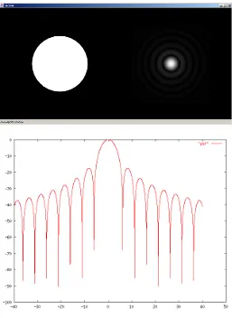
Figure 7.4. The top left shows a circular opening at the front of a telescope. The top right shows the corresponding Airy disk and a few diffraction rings. The plot on the bottom shows the cross-sectional intensity on alogscale. The desired level of10−10

corresponds to an intensity level of−100on this log plot. It is way off to the side. It occurs out somewhere around the

meter diameter. That is more than 10 times the diameter of the mirror in the Hubble space telescope. There are not any rockets in existence, or on the drawing boards, that will be capable of lifting such a large monolithic object into space at any time in the foreseeable future. For this reason some clever ideas are required. A few have been proposed. Perhaps the most promising one exploits the idea that the ring pattern is a consequence of the circular shape of the telescope. Different shapes provide different patterns—perhaps some of them provide a very dark zone very close to the Airy disk. An even broader generalization is to consider a telescope that has a filter over its opening that has light transmission properties that vary over the surface of the filter. If the transmission is everywhere either zero or one then the filter acts to create a different shaped opening. Such filters are calledapodizations. The problem is to find an apodization that provides a very dark area very close to the Airy disk. Okay, enough with the words already—we need to give a mathematical formulation of the problem. The diffraction pattern produced by the star in the image is the square of the electric field at the image plane and the electric field at the image plane turns out to be just the Fourier transform of the apodization functionAdefining the transmissivity of the apodized pupil:

E(ξ, ζ) = Z Z

S

e−2πi(xξ+yζ)A(x, y)dxdy,

where

S ={(x, y) : 0≤r(x, y)≤1/2, θ(x, y)∈[0,2π]},

andr(x, y)andθ(x, y)denote the polar coordinates associated with point(x, y). Here, and throughout this section, x and y denote coordinates on the filter measured in units of the mirror diameterDandξandζdenote angular (radian) deviation from on-axis measured in units of wavelengthλover mirror-diameter (λ/D) or, equivalently, physical distance in the image plane measured in units of focal-length times wavelength over mirror-diameter (f λ/D).

For circularly-symmetric apodizations, it is convenient to work in polar co-ordinates. To this end, letr andθdenote polar coordinates in the filter plane and letρandφdenote the image plane coordinates:

x = rcosθ ξ = ρcosφ y = rsinθ ζ = ρsinφ.

Hence,

The electric field in polar coordinates depends only onρand is given by

E(ρ) = Z 1/2

0

Z 2π

0

e−2πirρcos(θ−φ)A(r)rdθdr, (7.4)

= 2π

Z 1/2

0

J0(2πrρ)A(r)rdr, (7.5)

whereJ0denotes the0-th order Bessel function of the first kind. Note that the mapping from apodization functionAto electric fieldEis linear. Furthermore, the electric field in the image plane is real-valued (because of symmetry) and its value atρ= 0is thethroughputof the apodization:

E(0) = 2π

Z 1/2

0

A(r)rdr.

As mentioned already, the diffraction pattern, which is called thepoint spread function(psf), is the square of the electric field. The contrast requirement is that the psf in the dark region be10−10_{of what it is at the center of the Airy disk.} Because the electric field is real-valued, it is convenient to express the contrast requirement in terms of it rather than the psf, resulting in a field requirement of

±10−5.

The apodization that maximizes throughput subject to contrast constraints can be formulated as an infinite dimensional linear programming problem:

maximize E(0)

subject to ₋10−5E(0)_≤E(ρ)_≤10−5_{E(0), ρ}

iwa≤ρ≤ρowa,

0≤A(r)≤1, 0≤r≤1/2,

whereρiwadenotes a fixedinner working angleandρowaa fixedouter working

angle. Discretizing the sets ofr’s andρ’s and replacing the integrals with their Riemann sums, the problem is approximated by a finite dimensional linear programming problem that can be solved to a high level of precision.

The solution obtained forρiwa = 4 andρowa = 40 is shown in Figure 7.5.

0 0.2 0.4 0.6 0.8 1

0 0.05 0.1 0.15 0.2 0.25 0.3 0.35 0.4 0.45 0.5

Figure 7.5. The optimal apodization function turns out to be of bang-bang type.

rings:

[r0, r1] first opening

[r2, r3] second opening

[r4, r5] third opening ..

.

[r2m−2, r2m−1] m-th opening

With this notation, the formula forE(ρ) given in (7.5) can be rewritten as a sum of integrals over these openings:

E(ρ) = 2π

m−1

X

k=0

Z r2k+1

r2k

J0(2πrρ)rdr,

= 1

ρ

m−1

X

k=0

Treating therk’s as variables and using this new expression for the electric field,

the mask design problem becomes:

maximize π

m−1

X

k=0

r2_2k+1−r₂2_k

subject to ₋10−5E(0)_≤E(ρ)_≤10−5E(0), ρiwa ≤ρ≤ρowa,

0_≤r0 ≤r1≤ · · · ≤r2m−1 ≤1/2.

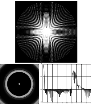
This problem is a nonconvex nonlinear optimization problem and hence the best hope for solving it in a reasonable amount of cpu time is to use a “local-search” method starting the search from a solution that is already close to optimal. The bang-bang solution from the linear programming problem can be used to generate a starting solution. Indeed, the discrete solution to the linear programming problem can be used to find the inflection points ofAwhich can be used as initial guesses for therk’s. loqowas used to perform this local optimization. Figure 7.6 shows an optimal concentric-ring mask computed using an inner working angle of4and an outer working angle of60. Using this mask over a10meter primary mirror makes it possible to image the Earth-like planet30light-years away from us. Even a telescope with a10meter primary mirror is larger than anything we have launched into space to date but it is a size that fits into the realm of possibility. And, if a10circular mirror is too large, we could fall back on elliptical designs say using a4_×10mirror. Such a mirror could be put into space using currently available Delta rockets. The mask designs presented here and many others can be found in the following references: ref:Spergel; ref:kasdin; KVSL02; VSK02; VSK03.

4.

Minimum weight truss design

0 10 20 30 40 50 60 70 80 90 100 10-15

10-10

10-5

100

Figure 7.6. At the top is shown the concentric ring apodization. The second row shows the psf as a 2-D image and in cross-section. Note that it achieves the required10−10

3

1 2

4 5

b₁ b₂

b₅

u₂₁

u₂₄ u₂₃

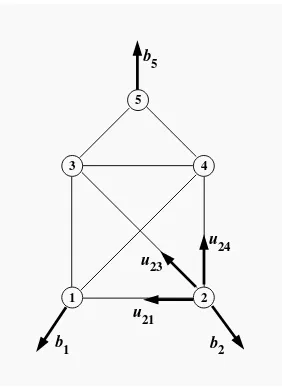
Figure 7.7. A design space showing5nodes and8arcs. Also shown are three externally applied forces and the tensile forces they induce in node2.

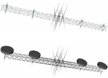
be launchable into space yet stiff enough that it can hold four massive telescopes in position with a precision that is small relative to the wavelength of light.

Such truss optimization problems have a long history starting, I believe, with Jim Ho’s Ph.D. thesis at Stanford which was published in Ho75. In more recent times, Ronnie Ben-Tal has collaborated with Bendsøe and Zowe on just this family of problems. They wrote many papers including the seminal paper BBZ94. Anyway, in the following subsection, I will outline the basic optimization problem and its reduction to a linear programming problem. Then in the following subsection, I will describe how it is being applied to the truss-design problem mentioned above.

Mathematical Formulation

We assume we are given a design space, which consists of a set_N of nodes (aka joints) at fixed locations and a setA of undirected arcs (aka members) connecting various pairs of nodes—see Figure 7.7. The unknowns in the prob-lem are the tensionsxij in each member. We assume that there are many more

members than are needed to make a rigid truss, so it follows that the system is underdetermined and there is lots of freedom as to how the forces “flow” through the structure. The tensionsxij are allowed to go negative. Negative

force balance equations are:

To write down the equations in more generality, we need to introduce some notation:

pi = position vector for jointi

uij =

pj−pi

kpj−pik

Note thatuji = −uij. With these notations, the general force balance

con-straints can be written as

X

j:

{i,j}∈A

uijxij =−bi, i= 1, . . . , m

It is instructive to write these equations in matrix form asAx=₋b, where

xT =

would be exactly a node-arc incidence matrix. In fact, much of the theory that has been developed for minimum-cost network flow problems has an immediate analogue in these truss design problems. These connections are described at length in Van01.

we assume that they are equal). Hence, the minimum weight structural design problem can be formulated like this:

minimize X

{i,j}∈A

lij|xij|

subject to X

j:

{i,j}∈A

uijxij =−bi i= 1,2, . . . , m.

This is not quite a linear programming problem. But it is easy to convert it into one using a common trick of splitting every variable into the difference between its positive and negative parts:

xij = x+_ij −x−_ij, x_ij+, x−_ij ≥0, x+_ijx−_ij = 0

|xij| = x+ij +x−ij

In terms of these new variables, the problem can be written as follows:

minimize X

{i,j}∈A

(lijx+ij+lijx−ij)

subject to X

j:

{i,j}∈A

(uijx+_ij−uijx−_ij) =−bi i= 1,2, . . . , m

x+_ijx−_ij= 0 {i, j} ∈ A, x+_ij, x−_ij≥0 _{i, j_{} ∈ A}.

It is easy to argue that one can drop the complementarity type constraints,

x+_ijx−_ij = 0,_{i, j_{} ∈ A}, since these constraints will automatically be satisfied at optimality. With these constraints gone, the problem is a linear programming problem that can be solved very efficiently.

It was shown in BBZ94 that this minimum weight structural design problem is dual to a maximum stiffness structural design problem and therefore that the structure found according to this linear programming methodology is in fact maximally stiff.

Telescope Truss Design

param m default 26; param n default 39;

set X := {0..n}; set Y := {0..m};

set NODES := X cross Y; # A lattice of Nodes

set ANCHORS within NODES

:= { x in X, y in Y : x == 0 && y >= floor(m/3) && y <= m-floor(m/3) };

param xload {(x,y) in NODES: (x,y) not in ANCHORS} default 0; param yload {(x,y) in NODES: (x,y) not in ANCHORS} default 0;

param gcd {x in -n..n, y in -n..n} := (if x < 0 then gcd[-x,y] else (if x == 0 then y else

(if y < x then gcd[y,x] else (gcd[y mod x, x]) )));

set ARCS := { (xi,yi) in NODES, (xj,yj) in NODES: abs(xj-xi) <= 3 && abs(yj-yi) <=3 &&

abs(gcd[ xj-xi, yj-yi ]) == 1 && ( xi > xj || (xi == xj && yi > yj) ) };

param length {(xi,yi,xj,yj) in ARCS} := sqrt( (xj-xi)^2 + (yj-yi)^2 );

var comp {ARCS} >= 0; var tens {ARCS} >= 0; minimize volume:

sum {(xi,yi,xj,yj) in ARCS}

length[xi,yi,xj,yj] * (comp[xi,yi,xj,yj] + tens[xi,yi,xj,yj]);

subject to Xbalance {(xi,yi) in NODES: (xi,yi) not in ANCHORS}: sum { (xi,yi,xj,yj) in ARCS }

((xj-xi)/length[xi,yi,xj,yj]) * (comp[xi,yi,xj,yj]-tens[xi,yi,xj,yj]) +

sum { (xk,yk,xi,yi) in ARCS }

((xi-xk)/length[xk,yk,xi,yi]) * (tens[xk,yk,xi,yi]-comp[xk,yk,xi,yi]) = xload[xi,yi];

subject to Ybalance {(xi,yi) in NODES: (xi,yi) not in ANCHORS}: sum { (xi,yi,xj,yj) in ARCS }

((yj-yi)/length[xi,yi,xj,yj]) * (comp[xi,yi,xj,yj]-tens[xi,yi,xj,yj]) +

sum { (xk,yk,xi,yi) in ARCS }

((yi-yk)/length[xk,yk,xi,yi]) * (tens[xk,yk,xi,yi]-comp[xk,yk,xi,yi]) = yload[xi,yi];

let yload[n,m/2] := -1;

solve;

Figure 7.9. Top.The design space.Bottom.The optimal design.

three principle axes of rotation. Torques are modeled as pairs of forces that are equal and opposite but applied at points that are not colinear with the direction of the force. So, our basic model has six load scenarios. Forces must be balanced in each scenario. Of course, the tensions/compressions are scenario dependent but the beam cross-sections must be chosen independently of the scenario (since one physical structure must be stiff under each scenario).

5.

New orbits for the

n

-body problem

Since the time of Lagrange and Euler precious few solutions to then-body problem have been discovered. Lagrange proved that two bodies being mutually attracted to the other by gravity will execute elliptical orbits where each of the two ellipses has a focus at the center of mass of the two-body system. This can be proved mathematically. Not only does this solution to Newton’s equations of motion exist, but it is also stable. Euler pointed out that a third body can be placed stationarily at the center of mass and this makes a solution to the three-body problem. However, this 3-body system is unstable—if the third body is perturbed ever so slightly the whole system will fall apart. A few other simple solutions have been known for hundreds of years. For example, you can distributenequal-mass bodies uniformly around a circle and start each one off with a velocity perpendicular to the line through the center and this system will behave much like the2-body system. But, for three bodies or more, this system is again unstable. So, it was a tremendous shock a few years ago when Cris Moore at the Sante Fe Institute discovered a new, stable solution to the equal-mass3-body problem. This discovery has created a tremendous level of interest in the celestial mechanics community. Not only was the solution he discovered both new and stable, it is also aesthetically beautiful because each of the three bodies follow the exact same path. At any given moment they are at different parts of this path. Such orbital systems have been calledchoreographies. Many celestial mechanics have been working hard to discover new choreographies. The interesting thing for us is that the main tool is to minimize the so-called action functional.

In this section, we will describe how it is that minimizing the action functional provides solutions to then-body problem and we will illustrate several new solutions that we have found.

Least Action Principle

Given n bodies, letmj denote the mass and zj(t) denote the position in

R2 ₌ C _{of body j at timet. The action functional is a mapping from the} space of all trajectories,z1(t), z2(t), . . . , zn(t),0≤t≤2π, into the reals. It is

defined as the integral over one period of the kinetic minus the potential energy:

A= Z 2π

0



 X

j

mj 2 kz˙jk

2₊ X j,k:k<j

mjmk

kzj−zkk 

dt.

variation of the action functional,

Note that ifmj = 0 for some j, then the first order optimality condition

reduces to 0 = 0, which isnot the equation of motion for a massless body. Hence, we must assume that all bodies have strictly positive mass.

Periodic Solutions

Our goal is to use numerical optimization to minimize the action functional and thereby find periodic solutions to then-body problem. Since we are in-terested only in periodic solutions, we express all trajectories in terms of their Fourier series:

Abandoning the efficiency of complex-variable notation, we can write the tra-jectories with componentszj(t) = (xj(t), yj(t))andγk= (αk, βk).So doing,

Since we plan to optimize over the space of trajectories, the parametersa0,ac_k,

as_k, b0, bck, and bsk are the decision variables in our optimization model. The

param N := 3; # number of masses

param n := 15; # number of terms in Fourier series representation param m := 100; # number of terms in numerical approx to integral

set Bodies := {0..N-1};

set Times := {0..m-1} circular; # "circular" means that next(m-1) = 0

param theta {t in Times} := t*2*pi/m; param dt := 2*pi/m;

param a0 {i in Bodies} default 0; param b0 {i in Bodies} default 0; var as {i in Bodies, k in 1..n} := 0; var bs {i in Bodies, k in 1..n} := 0; var ac {i in Bodies, k in 1..n} := 0; var bc {i in Bodies, k in 1..n} := 0;

var x {i in Bodies, t in Times}

= a0[i]+sum {k in 1..n} ( as[i,k]*sin(k*theta[t]) + ac[i,k]*cos(k*theta[t]) ); var y {i in Bodies, t in Times}

= b0[i]+sum {k in 1..n} ( bs[i,k]*sin(k*theta[t]) + bc[i,k]*cos(k*theta[t]) );

var xdot {i in Bodies, t in Times} = (x[i,next(t)]-x[i,t])/dt; var ydot {i in Bodies, t in Times} = (y[i,next(t)]-y[i,t])/dt;

var K {t in Times} = 0.5*sum {i in Bodies} (xdot[i,t]^2 + ydot[i,t]^2);

var P {t in Times}

= - sum {i in Bodies, ii in Bodies: ii>i}

1/sqrt((x[i,t]-x[ii,t])^2 + (y[i,t]-y[ii,t])^2);

minimize A: sum {t in Times} (K[t] - P[t])*dt;

let {i in Bodies, k in 1..n} as[i,k] := 1*(Uniform01()-0.5); let {i in Bodies, k in 1..n} ac[i,k] := 1*(Uniform01()-0.5); let {i in Bodies, k in n..n} bs[i,k] := 0.01*(Uniform01()-0.5); let {i in Bodies, k in n..n} bc[i,k] := 0.01*(Uniform01()-0.5);

solve;

Figure 7.10 shows theamplprogram for minimizing the action functional. Note that the action functional is a nonconvex nonlinear functional. Hence, it is expected to have many local extrema and saddle points. We use the author’s local optimization software calledloqo(see SOR9708, Van97d) to find local minima in a neighborhood of an arbitrary given starting trajectory. One can provide either specific initial trajectories or one can give random initial trajec-tories. The four lines just before the call tosolvein Figure 7.10 show how to specify a random initial trajectory. Of course,amplprovides capabilities of printing answers in any format either on the standard output device or to a file. For the sake of brevity and clarity, the print statements are not shown in Figure 7.10. amplalso provides the capability to loop over sections of code. This is also not shown but the program we used has a loop around the four initialization statements, the call to solve the problem, and the associated print statements. In this way, the program can be run once to solve for a large number of periodic solutions.

Choreographies. Recently, CM00 introduced a new family of solutions to then-body problem called choreographies. Achoreographyis defined as a solution to then-body problem in which all of the bodies share a common orbit and are uniformly spread out around this orbit. Such trajectories are even easier to find using the action principle. Rather than having a Fourier series for each orbit, it is only necessary to have one master Fourier series and to write the action functional in terms of it. Figure 7.11 shows theamplmodel for finding choreographies.

Stable vs. Unstable Solutions

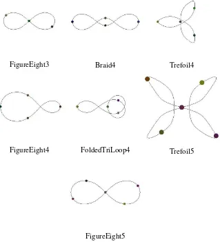
Figure 7.12 shows some simple choreographies found by minimizing the action functional using theamplmodel in Figure 7.11. The famous3-body figure eight, first discovered by Mor93 and later analyzed by CM00, is the first one shown—labeled FigureEight3. It is easy to find choreographies of arbitrary complexity. In fact, it is not hard to rediscover most of the choreographies given in CGMS01, and more, simply by putting a loop in theamplmodel and finding various local minima by using different starting points.

However, as we discuss in a later section, simulation makes it apparent that, with the sole exception of FigureEight3, all of the choreographies we found are unstable. And, the more intricate the choreography, the more unstable it is. Since the only choreographies that have a chance to occur in the real world are stable ones, many cpu hours were devoted to searching for other stable choreographies. So far, none have been found. The choreographies shown in Figure 7.12 represent the ones closest to being stable.

param N := 3; # number of masses

param n := 15; # number of terms in Fourier series representation

param m := 99; # terms in num approx to integral. must be a multiple of N

param lagTime := m/N;

set Bodies := {0..N-1};

set Times := {0..m-1} circular; # "circular" means that next(m-1) = 0

param theta {t in Times} := t*2*pi/m; param dt := 2*pi/m;

param a0 default 0; param b0 default 0; var as {k in 1..n} := 0; var bs {k in 1..n} := 0; var ac {k in 1..n} := 0; var bc {k in 1..n} := 0;

var x {i in Bodies, t in Times}

= a0+sum {k in 1..n} ( as[k]*sin(k*theta[(t+i*lagTime) mod m]) + ac[k]*cos(k*theta[(t+i*lagTime) mod m]) ); var y {i in Bodies, t in Times}

= b0+sum {k in 1..n} ( bs[k]*sin(k*theta[(t+i*lagTime) mod m]) + bc[k]*cos(k*theta[(t+i*lagTime) mod m]) );

var xdot {i in Bodies, t in Times} = (x[i,next(t)]-x[i,t])/dt; var ydot {i in Bodies, t in Times} = (y[i,next(t)]-y[i,t])/dt;

var K {t in Times} = 0.5*sum {i in Bodies} (xdot[i,t]^2 + ydot[i,t]^2);

var P {t in Times}

= - sum {i in Bodies, ii in Bodies: ii>i}

1/sqrt((x[i,t]-x[ii,t])^2 + (y[i,t]-y[ii,t])^2);

minimize A: sum {t in Times} (K[t] - P[t])*dt;

let {k in 1..n} as[k] := 1*(Uniform01()-0.5); let {k in 1..n} ac[k] := 1*(Uniform01()-0.5); let {k in n..n} bs[k] := 0.01*(Uniform01()-0.5); let {k in n..n} bc[k] := 0.01*(Uniform01()-0.5);

solve;

FigureEight3 Braid4 Trefoil4

FigureEight4 FoldedTriLoop4 Trefoil5

FigureEight5

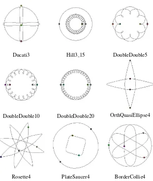
Ducati3 Hill3 15 DoubleDouble5

DoubleDouble10 DoubleDouble20 OrthQuasiEllipse4

Rosette4 PlateSaucer4 BorderCollie4

model from Figure 7.10. The most interesting such solutions are shown in Figure 7.13. The one labeled Ducati3 is stable as are Hill3 15 and the three DoubleDouble solutions. However, the more exotic solutions (OrthQuasiEl-lipse4, Rosette4, PlateSaucer4, and BorderCollie4) are all unstable.

For the interested reader, ajavaapplet can be found at GravityApplet that allows one to watch the dynamics of each of the systems presented in this paper (and others). This applet actually integrates the equations of motion. If the orbit is unstable it becomes very obvious as the bodies deviate from their predicted paths.

Ducati3 and its Relatives

The Ducati3 orbit first appeared in Mor93 and has been independently redis-covered by this author, Broucke Bro03, and perhaps others. Simulation reveals it to be a stable system. Thejavaapplet at GravityApplet allows one to rotate the reference frame as desired. By setting the rotation to counter the outer body in Ducati3, one discovers that the other two bodies are orbiting each other in nearly circular orbits. In other words, the first body in Ducati3 is executing approximately a circular orbit, z1(t) = −eit, the second body is oscillating back and forth roughly along thex-axis,z2(t) = cos(t), and the third body is oscillating up and down they-axis,z3(t) =isin(t). Rotating so as to fix the first body means multiplying bye−it_:

¯

z1(t) = e−it(−eit) =−1

¯

z2(t) = e−itcos(t) = (1 +e−2it)/2

¯

z2(t) = e−itisin(t) = (1−e−2it)/2.

Now it is clear that bodies 2 and 3 are orbiting each other at half the distance of body 1. So, this system can be described as a Sun, Earth, Moon system in which all three bodies have equal mass and in which one (sidereal) month equals one year. The synodic month is shorter—half a year.

This analysis of Ducati3 suggests looking for other stable solutions of the same type but with different resonances between the length of a month and a year. Hill3 15 is one of many such examples we found. In Hill3 15, there are 15 sidereal months per year. Let Hill3ndenote the system in which there are

nmonths in a year. All of these orbits are easy to calculate and they all appear to be stable. This success suggests going in the other direction. Let Hill3 _n1 denote the system in which there arenyears per month. We computed Hill3 1₂ and found it to be unstable. It is shown in Figure 7.14.

In the preceding discussion, we decomposed these Hill-type systems into two2-body problems: the Earth and Moon orbit each other while their center of mass orbits the Sun. This suggests that we can find stable orbits for the

Hill3 2 Hill3 3 Hill3 0.5

Figure 7.14. Periodic Orbits—Hill-type with equal masses.

labeled DoubleDoublenare of this type. As already mentioned, these orbits are stable.

Given the existence and stability of FigureEight3, one often is asked if there is any chance to observe such a system among the stars. The answer is that it is very unlikely since its existence depends crucially on the masses being equal. The Ducati and Hill type orbits, however, are not constrained to have their masses be equal. Figure 7.15 shows several Ducati-type orbits in which the masses are not all equal. All of these orbits are stable. This suggests that stability is common for Ducati and Hill type orbits. Perhaps such orbits can be observed.

Limitations of the Model

The are certain limitations to the approach articulated above. First, the Fourier series is an infinite sum that gets truncated to a finite sum in the computer model. Hence, the trajectory space from which solutions are found is finite dimensional.

Second, the integration is replaced with a Riemann sum. If the discretization is too coarse, the solution found might not correspond to a real solution to the

n-body problem. The only way to be sure is to run a simulator.

Third, as mentioned before, all masses must be positive. If there is a zero mass, then the stationary points for the action function, which satisfy (7.6), don’t necessarily satisfy the equations of motion given by Newton’s law.

Ducati3 2 Ducati3 0.5 Ducati3 0.1

Ducati3 10 Ducati3 1.2 Ducati3 1.3

Ducati3 alluneq Ducati3 alluneq2

Elliptic Solutions

An ellipse with semimajor axisa, semiminor axisb, and having its left focus at the origin of the coordinate system is given parametrically by:

x(t) =f +acost, y(t) =bsint,

wheref =√a2_−b2_{is the distance from the focus to the center of the ellipse.} However, this isnotthe trajectory of a mass in the2-body problem. Such a mass will travel faster around one focus than around the other. To accommodate this, we need to introduce a time-change functionθ(t):

x(t) =f +acosθ(t), y(t) =bsinθ(t).

This functionθmust be increasing and must satisfyθ(0) = 0andθ(2π) = 2π. The optimization model can be used to find (a discretization of)θ(t) auto-matically by changingparam theta tovar theta and adding appropriate monotonicity and boundary constraints. In this manner, more realistic orbits can be found that could be useful in real space missions.

In particular, using an eccentricitye=f /a= 0.0167and appropriate Sun and Earth masses, we can find a periodic Hill-Type satellite trajectory in which the satellite orbits the Earth once per year.

References

M.P. Bendsøe, A. Ben-Tal, and J. Zowe. Optimization methods for truss geom-etry and topology design.Structural Optimization, 7:141–159, 1994. R. Broucke. New orbits for then-body problem. InProceedings of Conference

on New Trends in Astrodynamics and Applications, 2003.

A. Chenciner, J. Gerver, R. Montgomery, and C. Sim´o. Simple choreographic motions onnbodies: a preliminary study. InGeometry, Mechanics and Dy-namics, 2001.

A. Chenciner and R. Montgomery. A remarkable periodic solution of the three-body problem in the case of equal masses.Annals of Math, 152:881–901, 2000.

J.O. Coleman. Systematic mapping of quadratic constraints on embedded fir filters to linear matrix inequalities. InProceedings of 1998 Conference on Information Sciences and Systems, 1998.

J.O. Coleman and D.P. Scholnik. Design of Nonlinear-Phase FIR Filters with Second-Order Cone Programming. InProceedings of 1999 Midwest Sympo-sium on Circuits and Systems, 1999.

R. Fourer, D.M. Gay, and B.W. Kernighan.AMPL: A Modeling Language for Mathematical Programming. Scientific Press, 1993.

N.K. Karmarkar. A new polynomial time algorithm for linear programming. Combinatorica, 4:373–395, 1984.

N. J. Kasdin, D. N. Spergel, and M. G. Littman. An optimal shaped pupil coronagraph for high contrast imaging, planet finding, and spectroscopy. submitted to Applied Optics, 2002.

N.J. Kasdin, R.J. Vanderbei, D.N. Spergel, and M.G. Littman. Extrasolar Planet Finding via Optimal Apodized and Shaped Pupil Coronagraphs. Astrophys-ical Journal, 582:1147–1161, 2003.

M.S. Lobo, L. Vandenberghe, S. Boyd, and H. Lebret. Applications of second-order cone programming. Technical report, Electrical Engineering Depart-ment, Stanford University, Stanford, CA 94305, 1998. To appear inLinear Algebra and Applicationsspecial issue on linear algebra in control, signals and imaging.

I.J. Lustig, R.E. Marsten, and D.F. Shanno. Interior point methods for linear programming: computational state of the art.Operations Research Society of America Journal on Computing, 6:1–14, 1994.

C. Moore. Braids in classical gravity.Physical Review Letters, 70:3675–3679, 1993.

D. N. Spergel. A new pupil for detecting extrasolar planets.astro-ph/0101142, 2000.

R.J. Vanderbei. LOQO user’s manual—version 3.10. Optimization Methods and Software, 12:485–514, 1999.

R.J. Vanderbei. http://www.princeton.edu/_∼rvdb/JAVA/astro/galaxy/Galaxy.html, 2001. .

R.J. Vanderbei. Linear Programming: Foundations and Extensions. Kluwer Academic Publishers, 2nd edition, 2001.

R.J. Vanderbei and D.F. Shanno. An interior-point algorithm for nonconvex non-linear programming.Computational Optimization and Applications, 13:231– 252, 1999.

R.J. Vanderbei, D.N. Spergel, and N.J. Kasdin. Circularly Symmetric Apodiza-tion via Starshaped Masks.Astrophysical Journal, 599:686–694, 2003. R.J. Vanderbei, D.N. Spergel, and N.J. Kasdin. Spiderweb Masks for High

Contrast Imaging.Astrophysical Journal, 590:593–603, 2003.