An Assessment of Propensity Score
Matching as a Nonexperimental
Impact Estimator
Evidence from Mexico’s PROGRESA
Program
Juan Jose Diaz
Sudhanshu Handa
a b s t r a c t
Not all policy questions can be addressed by social experiments.
Nonexperimental evaluation methods provide an alternative to experimental designs but their results depend on untestable assumptions. This paper pre-sents evidence on the reliability of propensity score matching (PSM), which estimates treatment effects under the assumption of selection on observables, using a social experiment designed to evaluate the PROGRESA program in Mexico. We find that PSM performs well for outcomes that are measured comparably across survey instruments and when a rich set of control vari-ables is available. However, even small differences in the way outcomes are measured can lead to bias in the technique.
I. Introduction
Although social experiments are the benchmark method for estimating the impact of social programs, experiments are seldom available because they are costly, raise ethical concerns due to the denial of potentially beneficial treatment to qualified
Juan Jose Diaz is an economist at the Group for the Analysis of Development (GRADE) in Lima, Peru. Sudhanshu Handa is associate professor in the Department of Public Policy at the University of North Carolina at Chapel Hill and fellow at the Carolina Population Center. This paper could not have been written without the assistance of Monica Orozco of PROGRESA, who provided essential data and explained operational details of the program to us. The authors thank Jeff Smith and an anonymous reviewer for constructive comments on earlier versions of this manuscript. The data used in this paper are available from Progresa in Mexico City. Other scholars wishing for guidance about how to apply for the data may contact Handa at shanda@email.unc.edu.
[Submitted July 2004; accepted August 2005]
individuals, and are often infeasible for universal entitlements or ongoing programs.1 Consequently, testing the reliability of nonexperimental methods is a central issue in the program evaluation literature. Nonexperimental methods identify program impacts by imposing untestable assumptions on behavior. Randomized experiments, when avail-able, can be used to assess the validity of those assumptions and thus the performance of alternative nonexperimental techniques of impact evaluation.
This study contributes to the small but growing literature on the performance of one particular type of nonexperimental technique, propensity score matching (PSM), which estimates treatment effects under the maintained assumption of selection on observables. PSM is computationally simple to implement and is increasingly being used to evaluate social programs, particularly employment and training programs (Larsson 2003; Levine and Painter 2003; Sianesi 2004). Our assessment of PSM is done with a unique data set from a Mexican social experiment designed to evaluate that country’s new poverty program, PROGRESA, a conditional cash transfer pro-gram targeted to poor rural households.
The PROGRESA program has national coverage and is mandatory; all households in participant localities that satisfy program eligibility rules and comply with its requirements receive treatment. Eligible households receive benefits provided they enroll their children in school, send them for health checkups, and at least one adult attends a monthly health talk. The program expanded in phases beginning in late 1997, and by 2000 was operating in all 31 states across Mexico covering approxi-mately 2.6 million rural households. To evaluate the impacts of the program a ran-domized experiment was carried out during the second phase of incorporation. Five hundred and six program-eligible localities in seven Mexican states were included in the evaluation, of which approximately one-third were randomly selected for delayed entry into the program and thus served as the randomized out “control” group for the impact evaluation.
We combine the PROGRESA experimental data (ENCEL) with a Mexican national household survey on income and expenditure (ENIGH) and then use a variety of PSM methods to select a comparison group from ENIGH. We compare outcomes from this nonexperimental comparison group with those from the actual experimental control group to assess the potential bias that arises when estimating program impacts using matching methods. We focus on three important program-related outcomes: food expenditures, teenage school enrollment, and child labor. Of these three outcomes, the latter two are measured consistently across the two different surveys, while food expenditures are measured differently. Specifically, the food expenditure module in ENIGH is longer and much more detailed than the comparable module in ENCEL, and is thus likely to pick up food expenditures that would otherwise be missed in ENCEL. This variation in survey instruments allows us to also assess the extent to which the performance of PSM is affected by differences in data measurement, an issue that has been highlighted in the literature on matching.
This paper contributes to the existing state of knowledge in several ways. First, all the published research on the reliability of PSM as an impact estimator is based on The Journal of Human Resources
320
employment and training programs inside the U.S.—ours is the first study to extend the evidence outside the United States and beyond employment programs. Second, we employ and compare a range of matching techniques including kernel and local-linear matching. Third, we are able to compare the bias in outcomes that are mea-sured similarly across survey instruments (school enrollment; child labor) with the bias in an outcome measured differently (food expenditure), thus providing evidence on the importance of questionnaire versus other sources of bias that might affect the performance of PSM.
Our main results show that PSM performs well for outcomes that are measured identically across surveys and when a rich set of covariates is available to estimate the propensity score. However, even small differences in the way outcomes are measured can lead to bias in the technique. We also find that using more stringent sample restrictions to eliminate potential bad matches does not solve the measurement prob-lem caused by different survey instruments, but does improve performance when working with a smaller set of covariates with which to estimate the propensity score.
II. Selected Literature
Most of the existing literature on the performance of PSM is based on social experiments from U.S. employment and training programs, either voluntary programs such as the National Supported Work Demonstration (NSW) and the National Job Training Partnership Act Study (JTPA) or mandatory programs such as the State Welfare-to-Work Demonstrations.2For voluntary interventions such as the JTPA, which are characterized by large pools of eligible candidates but a relatively small number of participants, the challenge of a nonexperimental evaluation strategy is to find nonparticipants in the same (or similar) labor market that look like partici-pants. In this context, selection bias arises mainly due to individual self-selection.
Using the JTPA experiment, Heckman, Ichimura, and Todd (1997, 1998) and Heckman et al. (1998) find that PSM performs well, provided researchers work with a rich set of control variables, use the same survey instruments, and compare partici-pants and nonparticipartici-pants from the same local labor market. Dehejia and Wahba (1999, 2002) use the NSW experiment combined with the CPS and PSID and show that PSM does well in replicating the experimental results. However, Smith and Todd (2005) show that the results in Dehejia and Wahba are particularly sensitive to their sample restrictions and that PSM actually exhibits considerable bias when applied to a less restrictive sample. This bias stems from differences in survey instruments as well as differences in local labor market conditions, although difference-in-difference matching is able to overcome the latter source of bias.
For mandatory interventions such as the welfare-to-work programs, the challenge for a nonexperimental study is to find welfare recipients from nonparticipant locations similar enough to welfare recipients from participant locations; thus, selection bias arises mainly because of geographic differences in labor markets. This is the type of
2. There is only one published paper to our knowledge that assesses the performance of nonexperimental evaluation techniques on something other than an employment program, and that is the Federal School Dropout Demonstration Assistance Program (SDDAP) (Agodini and Dynarski 2004).
selection bias most relevant to the PROGRESA evaluation. Assessments of PSM in this context are reported in Friedlander and Robins (1995) and Michalopoulos, Bloom, and Hill (2004), both of whom use experimental control units (or earlier cohorts) from one location as a nonexperimental comparison group for treatment units in a different location. Both studies conclude that substantial biases arise when com-paring recipients residing in different geographic areas, but that PSM helps in reduc-ing differences on pretreatment characteristics in out-of-state comparisons.
In summary, the PSM technique appears to perform better for voluntary programs relative to mandatory ones despite the fact that selection on unobservables is higher in the former case, and PSM only controls for selection on observables. However even the more optimistic results from voluntary programs indicate somewhat strict condi-tions for success—identical survey instruments, similar local labor market condicondi-tions, and a rich set of control variables.
III. The PROGRESA Program
In 1996, the Mexican government launched a new antipoverty program in rural areas, the Programa de Educación, Salud y Alimentación— PROGRESA,3which differed from previous national poverty programs in two key respects. First, it provided benefits conditional on beneficiaries fulfilling human cap-ital enhancing requirements: school enrollment of children aged 8–16, attendance by an adult at a monthly health seminar, and compliance by all family members to a schedule of preventive health checkups. Second, participants were identified using a very detailed targeting process aimed at reaching the poorest population in rural areas and avoiding local political influence in designating program beneficiaries.
A. Program Structure and Benefits
PROGRESA explicitly attempted to stimulate human capital investment and break the intergenerational cycle of poverty by setting the level of cash transfers according to the opportunity cost of children’s time. Thus, benefits increase according to the age of the child, starting at about $12 per month for primary school and increasing to $22 per month for middle school attendance, with girls receiving slightly higher subsidies (by about $2 per month) than boys. In addition to the schooling benefits, each eligi-ble household receives a fixed monthly payment of approximately $12 for food, and a lump sum for school uniforms and books ($13 per school semester). The average transfer represents about one-third of total monthly household income.
PROGRESA expanded in phases beginning in August 1997 when 3,369 localities covering 140,544 households were incorporated into the program. Phase 2 began in November 1997, incorporating 2,988 additional localities, and 160,161 households. By the end of Phase 11 in 2000, PROGRESA had incorporated more than 70,000 localities in all 31 states of the country, covering approximately 2.6 million rural households.
3. In 2000 the program expanded to cover poor urban communities and changed its name to Oportunidades.
Targeting of poor households was implemented centrally at the PROGRESA head-quarters in Mexico City and entailed three stages. First, all localities in the country were ranked using a “marginality index” constructed from 1990 National Census data; this index was stratified into five categories and localities in the bottom cate-gories (high and very high levels of marginality) were preselected to be part of the program. Out of 200,151 localities in Mexico, 76,098 rural localities (14.8 million people) were identified as having high or very high marginality levels and thus were preselected for the program.
In the second stage the program identified poor households within targeted locali-ties. A census was administered to all households in the selected localities to retrieve information about household characteristics that determined poverty status, including household income, which was used to identify households below the official poverty line. Predicted poverty status was then computed using the results from a discriminant analysis of the poverty indicator that selected the household characteristics that best discriminated between poor and nonpoor households. In general, the best predicting variables were a dependency index (number of children to number of working age adults); an overcrowding index (persons per bedroom); the sex, age, and schooling of the household head; the number of children; dwelling characteristics such as dirt floor, bathroom with running water, and access to electricity; and possession of durable goods such as a gas stove, a refrigerator, a washing machine, and a vehicle. These characteristics were used to compute the discriminant score that separated eligible and noneligible households within program localities.4
In Stage 3, the list of potential beneficiaries of the program was presented at a com-munity assembly for ratification. If the assembly rejected a household on the list or an omitted household was alleged to be poor a review of that case was initiated by the central office.
B. The Social Experiment
The social experiment was launched during the second phase of implementation (November-December 1997) to evaluate the impacts of the program on outcomes such as health and schooling for children and household consumption. A total of 506 rural localities from seven states (Guerrero, Hidalgo, Michoacán, Puebla, Querétero, San Luis Potosi, and Veracruz) were selected for inclusion in the evaluation sample and 320 localities were randomly assigned to the treatment group while the remain-ing 186 localities were assigned to the control group.5All eligible households in treat-ment localities were immediately offered program benefits and services; none of those in the control localities received any benefit or service from the program until Phases 10 (November–December 1999) or 11 (March–April 2000) of expansion. Thus for eligible households in the control group localities, all program benefits were delayed for approximately 24 months.6
4. See Skoufias, Davis, and de la Vega (2001) for an assessment of the Progresa targeting procedure. 5. See Behrman and Todd (1999) for an assessment of the randomization process.
6. The impact evaluation of PROGRESA was conducted independently by the International Food Policy Institute (IFPRI) and an overview of the main results can be found in Skoufias (2000). All the evaluation studies are available on IFPRI’s website: www.ifpri.org/themes/progresa.htm.
IV. Methodology
A. Propensity Score MatchingThe parameter of interest in a program evaluation is the effect of treatment on the treated (TT), which compares the outcome of interest in the treated state (Y1) with the outcome in the untreated state (Y0) conditional on receiving treatment. The evaluation problem is that these outcomes cannot be observed for any single household in both states. Nonexperimental evaluation methods must make behavioral assumptions in order to identify the missing counterfactual. The key identifying assumption in the PSM technique is that outcomes are independent of program participation conditional on a particular set of observable characteristics. This is known as the conditional inde-pendence assumption or the assumption of selection on observables (Rosenbaum and Rubin (1983); Heckman and Robb (1985)).
Denoting by X the set of observables, the identification assumption can be expressed as Y0=D⎪P(X) where the symbol =denotes independence and P(X)is the propensity score. Actually, a weaker condition is required to identify the treatment parameter, that of conditional mean independence: E(Y0⎪D= 1,P(X)) = E(Y0⎪D= 0, P(X)). By conditioning on P(X) we can get an estimate of the unobserved component in the TTparameter. In particular, we can identify the parameter as follows:
(1) TT(X) = E(Y1⎪D= 1,P(X)) –E(Y0⎪D= 1,P(X)) = E(Y1⎪D= 1,P(X)) –E(Y0⎪D= 0,P(X)).
In our application below, we compute a direct measure of the bias associated with the
TT parameter instead of computing the parameter itself. We compare control units from the experimental data (ENCEL) with the nonexperimental comparison units from the national household survey (ENIGH). The estimated bias can thus be expressed as:
(2) B(X) = E(Y0⎪D= 1,P(X)) – {E(Y0⎪D= 0,P(X))}.
Control units Matched comparison units
Because control units do not receive any treatment, the estimated bias should be equal to zero. In this setting, any deviation from zero can be interpreted as evaluation bias. Our matching application is done in two steps. First, we combine background covariates from the experimental sample with these same variables for rural house-holds from the ENIGH, a nationally representative household survey, and estimate the probability of being selected to participate in the program (the probability of being eligible). Second, we apply PSM (Rosenbaum and Rubin 1983; Heckman, Ichimura, and Todd 1998) to the experimental control and nonexperimental comparison units to construct a matched comparison group from ENIGH, and then compare mean differ-ences in outcomes between the two groups.
B. Balancing Score and Balancing Test
We implement the matching procedure using a balancing score computed from a logit model. We use the log odds ratio as our balancing score because we are dealing with The Journal of Human Resources
choice-based samples where the proportion of the treatment group is oversampled in the data set. In practice we generate a dummy variable that takes a value of one when the observation comes from the experimental sample (either from the treatment or control groups) and zero when it comes from the nonexperimental sample. We esti-mate the logit model using all observations available (treatment, control, and non-experimental units) in order to gain efficiency, and then use the estimated coefficients to obtain the predicted probability (p) and the log odds ratio log (p/(1 −p)), for each observation in the control and comparison samples. Thus we are estimating the probabi-lity of being eligible conditional on a set Xof observable characteristics. Note that the variables used in Xare precisely the variables that PROGRESA uses in calculating its point score to determine household eligibility.
In the estimation of the propensity score we perform the balancing test described in Dehejia and Wahba (1999, 2002) to guide the specification of the logit model. This method essentially entails adding interaction and higher-order terms to our base model until tests for mean differences in covariates between control and comparison units become statistically insignificant.
C. Common Support
The common support is the region Swhere the balancing score has positive density for both treatment and comparison units. No matches can be formed to estimate the
TTparameter (or the bias) when there is no overlap between the treatment (control) and comparison groups. We define the region of common support by dropping obser-vations below the maximum of the minimums and above the minimum of the maxi-mums of the balancing score. This procedure entails some potential problems: the support condition may fail in interior regions; good matches could be lost near the boundary of the support region, and excluding observations in either group may change the parameter being estimated.
D. Matching Estimators
We examine the performance of several different matching methods. Applied to esti-mate the bias using control and comparison units, all matching estimators have the general form:
(3) Bm= n1
冱
Y冱
W i j Y( , )i I S n
i
j I S j
1 1 1 0
1
0
+ +
! = -! G
,
where Bmdenotes the matching estimator for the bias, n1denotes the number of obser-vations in the control sample, Y1irepresent the outcome for controls and Y0jrepresent
the outcome for comparison units, I1and I0denote the set of control and comparison units respectively, Srepresents the region of common support, and the term W(i, j) represent a weighting function that depends on the specific matching estimator. Aside from the commonly used nearest-neighbor method we provide results using three other matching estimators: caliper, kernel, and local linear matching. Caliper match-ing is a refinement of nearest neighbor that only allows a match within a specified dis-tance of the score of the treated unit and is a way to eliminate bad matches. The kernel
method uses a weighted average of all observations within the common support region; the farther away the comparison unit is from the treated unit the lower the weight. The weight we use is the normal (Gaussian) density. Local linear matching is similar to the kernel estimator but includes a linear term in the weighting function that is helpful when the data are asymmetric with respect to the balancing score. Formal expressions for each estimator are provided in the appendix. Finally, we use the boot-strap method to estimate standard errors for all of the matching estimators, which accounts for the fact that the balancing score is also estimated.
V. Data and Samples
A. SamplesThe PROGRESA experimental evaluation data (Encuesta de Evaluación de los Hogares-ENCEL) consists of four rounds of household surveys covering 506 locali-ties and approximately 25,000 households (poor and nonpoor). Surveys were con-ducted in March and October 1998, and May and November 1999. We use the October 1998 round of ENCEL, which corresponds to approximately 8–10 months of program participation for treated households. PROGRESA expanded in phases, beginning its intervention in the poorest localities. Households in the evaluation sam-ple were incorporated into the program during the second phase, and so are some of the poorest households in rural Mexico. This has important implications for the via-bility of the propensity score matching technique, which we discuss below.
The nonexperimental sample comes from the Encuesta Nacional sobre Ingresos y Gastos de los Hogares (ENIGH), a biannual nationally representative household survey that collects information on income, expenditures, household demographic composition, and school enrollment. The sample size is approximately 13,000 house-holds, of which approximately 4,000 are rural households; we use the 1998 round of ENIGH to construct the nonexperimental comparison group.
The 1998 wave of ENIGH was collected between September and early November, approximately 10–12 months after the start of PROGRESA, implying that some ENIGH households actually may have been participating in the program. Using PRO-GRESA retrospective administrative data, we are able to identify the date of entry (if entered) into the program for all rural localities that were sampled in ENIGH 1998. To avoid contamination bias we exclude all localities from the ENIGH rural sample that had already entered PROGRESA at the time of the survey. The resulting sample of rural households is what we refer to as Sample 1. In addition, because ENIGH is nationally representative and not poverty focused, many rural localities never entered PROGRESA because they did not qualify. Since households in localities that did not qualify for PROGRESA may not provide good matches for households in localities that did qualify, we also present estimates based on a restricted sample that excludes from Sample 1 all households in localities that never qualified for PROGRESA. We refer to this more restricted group of households as Sample 2. The benefit of using Sample 2 is that it allows us to see whether additional information on locality selec-tion, available only after a few years of program implementaselec-tion, is helpful in esti-mating program impact. On the other hand, excluding entire localities that never entered the program also risks excluding poor households within these communities The Journal of Human Resources
that might provide good matches. Indeed, a major concern of PROGRESA program managers is that the first stage in the targeting process excludes potential beneficiar-ies living in well-off localitbeneficiar-ies. In general, because ENIGH is nationally representa-tive while PROGRESA specifically targets the very poor, a big challenge is to see whether the matching technique is able to identify enough good matches from ENIGH to allow meaningful comparisons with the control group from ENCEL.
B. Differences in Questionnaire Design across Survey Instruments
Aside from differences in the sample frame that may inhibit good matches, a critical issue is the difference in questionnaire design between the two survey instruments (ENIGH and ENCEL). The expenditure module in ENIGH is much more detailed than the ENCEL, and while the surveys were fielded at around the same time of year, many of the recall periods are also different, so that differences in expenditure out-comes may be entirely due to questionnaire design rather than evaluation technique. On the other hand, the questions on individual school enrollment are comparable across surveys. Finally, the questions on employment are slightly more detailed in the ENIGH survey, with a few additional questions included to probe for paid employ-ment on the part of respondents. These differences allow us to assess whether the results are sensitive to variations in questionnaire design, a key issue pointed out by Heckman et al. (1998) and Smith and Todd (2005).
VI. Results
A. Mean Characteristics of Subample
The experimental data from ENCEL 1998-October consist of 7,703 treatment house-hold and 4,604 control househouse-holds. The nonexperimental data drawn from rural ENIGH-1998 consist of 3,837 households from which we extract the two working samples described above. Table 1 presents summary statistics on the control variables used in the logit regression to estimate the balancing score—these are the exact vari-ables used by PROGRESA in their targeting mechanism. Columns 1 and 2 provide means for the treatment and control units from ENCEL and these are virtually the same, indicating that control units in ENCEL are indeed a valid comparison group for the measurement of program impacts. The next three columns (Columns 3, 4, and 5) present means for, respectively, the entire ENIGH rural sample and the two working samples. Rural ENIGH households are clearly better off than their ENCEL counter-parts, as we would expect since ENIGH is nationally representative. For example, ENIGH household heads have significantly more schooling than ENCEL heads, sig-nificantly fewer children younger than age 13, and are more likely to have a refriger-ator, a gas stove, a washing machine, and a vehicle. Note that the mean characteristics in the ENIGH Sample 2 are closer to those of ENCEL, because we have excluded households from richer localities (those that never entered the program), although this sample is still clearly better off than the ENCEL controls. (Columns 6 and 7 will be discussed below.)
Table 2 presents the means for the outcome variables we consider in our applica-tion. This table has the same structure as Table 1 and presents average outcomes for
The Journal of Human Resources
328
Table 1
Summary Statistics for Conditioning Variables by Sample
Data set ENCEL ENIGH
Raw samples Matched samples
Sample Treatment Control All rural Sample1 Sample2 Sample1 Sample2
(1) (2) (3) (4) (5) (6) (7)
Demographic dependency 1.461 1.487 1.144 1.036 1.119 1.519 1.609
(0.95) (0.98) (1.05) (0.95) (1.04) (1.00) (1.15)
Head’s sex (female) 0.083 0.085 0.130 0.134 0.148 0.096 0.099
(0.28) (0.28) (0.34) (0.34) (0.36) (0.29) (0.30)
Head’s schooling
None 0.448 0.460 0.402 0.404 0.399 0.455 0.515
(0.50) (0.50) (0.49) (0.49) (0.49) (0.50) (0.50)
Incomplete primary 0.248 0.238 0.203 0.223 0.191 0.262 0.211
(0.43) (0.43) (0.40) (0.42) (0.39) (0.44) (0.41)
Incomplete secondary 0.055 0.055 0.104 0.120 0.091 0.040 0.054
(0.23) (0.23) (0.31) (0.32) (0.29) (0.20) (0.23)
Head’s age 42.204 42.529 47.141 47.210 47.421 41.509 41.699
(14.58) (14.88) (16.26) (16.37) (16.72) (14.11) (14.08)
Number of kids ages 13 2.457 2.489 1.488 1.341 1.431 2.567 2.541
Diaz and Handa
329
Crowding index 4.399 4.455 2.616 2.364 2.453 4.375 4.164
(2.26) (2.26) (1.86) (1.71) (1.69) (2.16) (1.99)
Do not have Social Security 0.969 0.960 0.821 0.776 0.867 0.955 0.962
(0.17) (0.20) (0.38) (0.42) (0.34) (0.21) (0.19)
No bathroom 0.482 0.489 0.346 0.289 0.412 0.568 0.525
(0.50) (0.50) (0.48) (0.45) (0.49) (0.50) (0.50)
Bathroom no water 0.500 0.493 0.482 0.478 0.452 0.417 0.452
(0.50) (0.50) (0.50) (0.50) (0.50) (0.49) (0.50)
Dirt floor 0.729 0.754 0.255 0.203 0.214 0.751 0.741
(0.44) (0.43) (0.44) (0.40) (0.41) (0.43) (0.44)
Without gas stove 0.847 0.834 0.362 0.260 0.285 0.842 0.837
(0.36) (0.37) (0.48) (0.44) (0.45) (0.37) (0.37)
Without refrigerator 0.959 0.962 0.559 0.474 0.566 0.960 0.971
(0.20) (0.19) (0.50) (0.50) (0.50) (0.20) (0.17)
Without washer 0.986 0.988 0.762 0.687 0.783 0.983 0.985
(0.12) (0.11) (0.43) (0.46) (0.41) (0.13) (0.12)
Without vehicle 0.979 0.980 0.789 0.737 0.773 0.941 0.942
(0.14) (0.14) (0.41) (0.44) (0.42) (0.24) (0.23)
Observations 7,703 4,604 3,837 2,438 724 765 371
The Journal of Human Resources
330
Table 2
Summary Statistics for Outcome Variables by Sample
ENCEL ENIGH
Mean
Difference All
Data set Treatment Control (1)-(2) Rural Sample 1 Sample 2 Sample 1 Sample 2
Sample (1) (2) (3) (4) (5) (6) (7) (8)
A. Household outcomes
Food expenditure per capita 511.8 476.7 35.0 909.7 970.7 880.8 695.9 646.6 (399.1) (405.2) (7.42) (697.8) (731.7) (664.7) (671.2) (619.4)
Observations 7,703 4,604 3,837 2,438 724 765 371
B. Children outcomes
School enrollment 13–16 0.546 0.480 0.066 0.582 0.581 0.509 0.475 0.396
(0.50) (0.50) (0.01) (0.49) (0.49) (0.50) (0.50) (0.49)
Observations 5,370 3,250 1,844 1,096 326 399 193
Work for pay 12–16 0.111 0.116 −0.005 0.107 0.121 0.124 0.114 0.111
(0.31) (0.32) (0.01) (0.31) (0.33) (0.33) (0.31) (0.32)
Observations 7,004 4,246 2,402 1,423 428 458 198
See notes to Table 1 for explanation of samples. Bold differences in Column 3 indicate statistical significance at 5 percent. Standard deviations in parentheses below mean.
the treatment and control units from ENCEL and the comparison units drawn from ENIGH samples. This table again shows that rural ENIGH households are signifi-cantly better-off than the ENCEL households, with signifisignifi-cantly higher per capita food expenditure and school enrollment rates for children aged 13–16. Notice once again that ENIGH Sample 2 displays means for food expenditure and school enroll-ment that are closer to the experienroll-mental controls (Column 2), since this sample excludes the group of “rich” localities that never entered the program. Finally, Column 3 displays the mean program impacts after only 8–10 months and show positive and significant differences for food expenditures and school enrollment only.
B. Balancing Score and Common Support
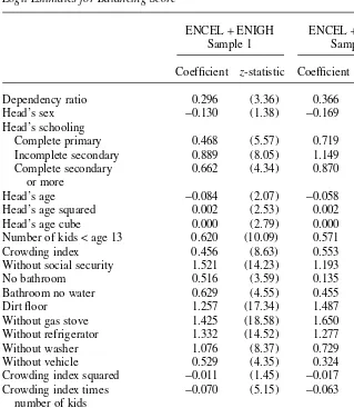
Results of the logit models to determine the probability of qualifying for the program are reported in Table A1 in the Appendix. For efficiency reasons these estimates are based on all households in the evaluation sample (households from both the treatment and control localities) and all rural households from either ENIGH Sample 1 or ENIGH Sample 2. The dependent variable is a dummy variable that takes a value of one when a household comes from the experimental data and zero when it comes from the nonexperimental sample.
A few differences are worth noting between the estimates over the two different samples. Almost all variables are significant when we use ENIGH Sample 1, which includes richer households, but several of these variables become insignificant when we use ENIGH Sample 2, where households are more homogenous due to the exclusion of these richer households. Furthermore, the coefficients on heads’ school-ing become much larger in the latter case, while the bathroom indicators become smaller.
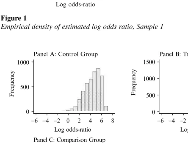
For each combined sample, we perform the balancing tests described earlier to assess the specification of the logit model used to estimate our balancing score. Based on these results we included quadratic terms for the dependency and crowding variable, as well as an interaction between crowding and the number of kids younger than age 13. Table A2 in the Appendix reports summary statistics on the estimated propensity score, the odds ratio, and the implied common support region—defined as the maximum of the minimums and the minimum of the maximums of the balanc-ing score between experimental and comparison units. The empirical distributions of the estimated odds ratios are shown graphically in Figures 1 and 2 for Samples 1 and 2 respectively.
When we use households from ENIGH Sample 1 as the comparison group, the mean odds ratio is −0.710 for ENIGH households and around 3.2 for both control and treatment households from ENCEL; 0.1 percent of the control group and 12.6 percent of the comparison group do not satisfy the common support criteria and are excluded from the subsequent analysis. In the case of ENIGH Sample 2, the mean odds ratio among the ENIGH sample is larger at 0.851 but still significantly lower than the mean for the ENCEL households, which is around 4.4. In this case imposing the common support criteria results in the elimination of 2.6 percent of the control and only 1 per-cent of the comparison groups; the latter number is naturally due to the screening out of “rich” households from this sample who would otherwise be excluded by the common support condition.
C. Matched Samples using Nearest-Neighbors
Columns 6 (Sample 1) and 7 (Sample 2) in Table 1 present average characteristics for the sample of households that have been matched on the balancing score using nearest-neighbor matching with replacement within the common support region. In both columns, mean characteristics are significantly different from the raw ENIGH samples before matching, and the matched households are clearly closer to ENCEL households in terms of those characteristics relative to the full rural ENIGH sample. For example, among the matched sample, the proportion of heads with incomplete secondary schooling is around 4–6 percent, compared with 5.5 percent in ENCEL and 10 percent in the overall rural sample from ENIGH. Similarly, the proportion of matched households without social security is 96 percent compared with 97 percent in ENCEL and 82 percent in overall rural ENIGH.
Mean outcomes for the matched households drawn from Samples 1 and 2 of ENIGH are reported in Columns 7 and 8 in Table 2. Average outcome values for these matched households are closer to the average outcomes for the experimental ENCEL households. Mean food expenditure is significantly lower in the matched samples ($696 and $647 respectively) relative to the full ENIGH samples in Columns 4–6, but these means are still quite large relative to the control group mean of $477 in Column 2. In the case of school enrollment, the nonexperimental comparison group means are 0.48 (Sample 1) and 0.40 (Sample 2) compared with 0.48 in the control group and 0.58 in the full rural ENIGH sample; notice that the matched Sample 2 mean is actu-ally lower that the control group mean. For child labor the matched sample means are 0.11 (in both Sample 1 and Sample 2) compared with 0.12 in the control group and 0.11 in the overall rural ENIGH.
D. Bias Estimates
Table 3 presents estimates of the bias for the three outcomes using various matching estimators. These estimates of bias are calculated by taking the difference in means between the control group from ENCEL and the nonexperimental comparison group from ENIGH. If matching does well in replicating the experimental control group then this difference should be zero. Thus, statistically significant deviations from zero (shown in bold in Table 3) indicate potential bias in impact estimates derived from the PSM technique. While our main objective is to compare PSM with the experimental estimates, it is of some interest to compare the PSM results with those from regres-sion analysis since the latter is a common nonexperimental technique. Using the sam-ple of control and comparison units only, we regress each of the outcomes on the same set of covariates used in the logit regression shown in Table A1, along with a “control group” dummy variable. The coefficient estimate of this dummy variable is reported as the regression-adjusted difference in Table 3. We also report the unadjusted or sim-ple mean difference in outcome between the control and comparison group.
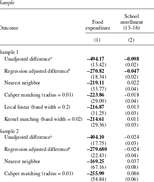
1. Results for Sample 1
The top panel of Table 3 presents estimates using ENIGH Sample 1, and these show that for food expenditures, all matching estimators lead to significant differences in The Journal of Human Resources
Diaz and Handa 333
Table 3
Direct Estimates of Bias for Alternative Matching Techniques by Outcome and Sample
School Work
Food enrollment for pay
Outcome expenditure (13–16) (12–16)
(1) (2) (3)
Sample 1
Unadjusted differencea
-494.17 -0.098 −0.006
(13.42) (0.02) (0.01)
Regression adjusted differenceb
-270.82 -0.047 −0.014
(18.34) (0.02) (0.01)
Nearest neighbor -219.11 0.022 −0.028
(33.77) (0.04) (0.03)
Caliper matching (radius = 0.01) -223.86 −0.018 0.011
(29.09) (0.04) (0.02)
Local linear (band width = 0.2) -216.87 0.013 -0.054
(31.25) (0.03) (0.02)
Kernel matching (band width = 0.02) -214.61 0.011 -0.041
(29.36) (0.03) (0.02)
Sample 2
Unadjusted differencea
-404.10 −0.024 −0.008
(17.75) (0.03) (0.02)
Regression adjusted differenceb
-279.680 −0.024 0.005
(22.43) (0.04) (0.02)
Nearest neighbor -169.25 0.037 0.012
(67.16) (0.08) (0.04)
Caliper matching (radius = 0.01) -255.99 0.086 0.031
(54.84) (0.06) (0.03)
Local linear (band width = 0.2) -239.39 0.030 0.046
(52.18) (0.06) (0.02)
Kernel matching (band width = 0.02) -264.56 0.047 0.021
(58.73) (0.06) (0.03)
Coefficient estimates represent the mean difference between the randomized out control observations and the matched comparison group sample, and indicate the bias in treatment effects using PSM. Each row is a dif-ferent estimation method. See Table 1 for definition of samples. Bootstrapped standard errors in parenthesis below the estimates account for the estimation of the propensity score (significant estimates at 5 percent shown in bold). The nearest-neighbor estimator was computed with replacement. The kernel estimator uses the normal density.
impact from the experimental results, with a downward bias ranging from 215 to 224 pesos. And while PSM outperforms regression for this outcome, the difference in bias between the two methods is only about 50 pesos, which is small relative to the overall size of the bias. Recall that there is significant variation in the data col-lection method for expenditures between the two surveys (ENCEL versus ENIGH), which may be driving the differences in the top panel of Column 1. Column 2 shows the results for school enrollment, which is measured identically across survey instruments. The point estimates indicate a potential bias of between negative two and positive two percentage points but none of these are statistically significant, indicating that for this outcome PSM is able to replicate the experimental result. On the other hand, simple regression methods show a statistically significant difference of 4.7 percentage points, implying that regression would lead to an underestimate of program impact for this outcome. Column 3 shows the results for child labor and these indicate some bias in the kernel and local linear matching techniques in the range of four to five percentage points. Here the negative coefficients imply an
overestimate of program impact (a lower rate of child work among beneficiaries). Recall that the questions on paid employment are more detailed in the ENIGH sur-vey and likely to lead to higher rates of reported child employment relative to ENCEL, which may explain the negative coefficients for the estimated bias in Column 3.
2. Results for Sample 2
Estimates based on the more restrictive comparison group from ENIGH Sample 2 are shown in the bottom panel of Table 3. These results follow the same general pattern as the top panel results for Sample 1, with a few exceptions. For example, there is a wider range of point estimates for the food expenditure bias across matching tech-niques, ranging from −169 for nearest neighbor to −265 for kernel, though all are sta-tistically significant. Consequently, several of the matching estimators are very close to the regression based estimate of bias of −280 pesos for this sample. In general for this particular outcome and regardless of the sample restriction, PSM techniques seem to provide little additional accuracy over regression techniques.
For school enrollment in Sample 2, neither the simple nor regression adjusted dif-ferences are statistically significant, implying that the sample restriction leads to the exclusion of households with better (higher) enrollment rates. This is also reflected in the point estimates of bias for the matching estimators in Column 2 which are all pos-itive, although none are statistically significant. Finally, the bottom panel of Column 3 indicates that local linear matching would still lead to significant bias in the impact estimate for child labor, although now the positive coefficient indicates a downward bias in program impact (lower child labor among the comparison group than is actu-ally the case among the randomized out controls).
The results from Table 3 suggest a few tentative conclusions. First, differences in the measurement of outcomes across survey instruments seem to strongly affect the performance of PSM. Second, the additional sample restriction (Sample 2) is not capable of solving the problem of differences in questionnaire design that exists for food expenditures, but does slightly improve the results for child labor.
E. Further Evidence on Questionnaire Bias
In this section we present additional evidence on the importance of questionnaire design for the performance of PSM. As mentioned earlier, we are able to identify the date of entry into PROGRESA (if entered) of all rural localities in the ENIGH data. For the localities that entered the program, PROGRESA officials have predicted pro-gram participants by applying the targeting algorithm to all households in the ENIGH data residing in program localities. Although this is not the same as identifying actual program participants through administrative records, program takeup rates are almost universal so that this method is likely to give us a very good idea about which ENIGH households are actually participating in the program. In our data we identify just over 1,000 households (27 percent of the rural sample) that live in program localities and
qualify for eligibility according to the targeting algorithm.
Our approach is to use these households as the treatment group, draw a matched comparison group from the remaining ENIGH households, and calculate impact esti-mates for the three outcomes. Since we are now working off the same survey instru-ment, we would expect to see impact estimates for food expenditure that are either in line with those from the experiment, or that are “off” by an amount that is signifi-cantly smaller than the 220 peso range reported in Column 1 of Table 3 if those results are indeed driven by questionnaire bias. In addition, we would expect the PSM impact estimates for enrollment and child labor to be in line with the experimental estimates since the results in Table 3 suggest that PSM can (with a few exceptions for child labor) replicate the social experiment.
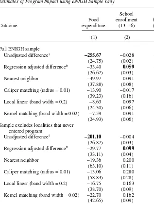
The results of this exercise are presented in the top panel of Table 4, where the first two rows once again display the unadjusted and regression-adjusted differences. Note that these coefficients are impact estimates and cannot be directly compared with the results in Table 3, but rather to the experimental impact shown at the bottom of the table (which are taken from Column 3 of Table 2). The PSM impact estimates for food expenditure in Column 1 are negative and range from 50 to 8 pesos but are all statistically insignificant, indicating no program impact. The implied bias in these estimates ranges from 85 to 43 pesos (calculated as the distance between the PSM impact estimate and the experimental impact estimate), or about one-fourth of the bias estimates reported in Column 1 of Table 3 which hover around the 220 peso mark. This implies that around 75 percent of the bias in Column 1 of Table 3 is accounted for by differences in survey instruments.
The top panel of Column 2 in Table 4 shows the impact estimates for school enroll-ment, and with the exception of caliper matching these are around nine percentage points, compared with the experimental impact of seven points. The PSM estimates tend to be insignificant at 5 percent but this is likely due to the smaller sample sizes in this analysis (the local linear and kernel estimates are significant at 15 percent). The impact estimates for child labor are shown in Column 3 and these are all statistically insignificant as is the experimental estimate at the bottom of that column, although some of the point estimates are fairly large. However for this outcome PSM outper-forms regression which shows a significant program effect of four percentage points. The bottom panel of Table 4 presents the results after excluding households in localities that never entered the program (this is equivalent to Sample 2 that we
The Journal of Human Resources 336
Table 4
Estimates of Program Impact using ENIGH Sample Only
School Work
Food enrollment for pay
Outcome expenditure (13–16) (12–16)
(1) (2) (3)
Full ENIGH sample Unadjusted differencea
-255.67 −0.028 -0.031
(24.75) (0.02) (0.01)
Regression adjusted differenceb −33.40 0.059
-0.040
(26.67) (0.03) (0.02)
Nearest neighbor −49.97 0.091 −0.055
(37.88) (0.08) (0.06)
Caliper matching (radius = 0.01) −13.90 −0.017 −0.006
(39.23) (0.16) (0.09)
Local linear (band width = 0.2) −8.63 0.097 −0.049
(24.30) (0.06) (0.03)
Kernel matching (band width = 0.02) −7.59 0.091 −0.050
(24.93) (0.06) (0.03)
Sample excludes localities that never entered program
Unadjusted differencea
-201.10 −0.004 −0.024
(26.87) (0.03) (0.02)
Regression adjusted differenceb −29.77 0.099 −0.020
(33.11) (0.04) (0.02)
Nearest neighbor −19.36 0.200 −0.025
(63.10) (0.11) (0.08)
Caliper matching (radius = 0.01) −13.06 0.280 −0.163
(58.83) (0.28) (0.18)
Local linear (band width = 0.2) −16.75 0.163 −0.014
(38.70) (0.09) (0.06)
Kernel matching (band width = 0.02) −22.70 0.162 −0.024
(42.65) (0.09) (0.06)
Experimental impact
Unadjusted differencec 35.0 0.066 −0.005
(7.42) (0.01) (0.01)
Coefficients are average treatment effects using households from rural ENIGH only.
a. Mean difference between Progresa and non-Progresa households in the relevant ENIGH sample. b. OLS coefficient of the treatment dummy estimated on the relevant ENIGH sample and including all other covariates.
describe earlier). The range of estimates for food expenditure is much smaller in this sample, and the implied bias is now between 57 and 48 pesos (these are always under-estimates), again representing about 25 percent of the bias in Table 3 and implying that the remaining 75 percent is due to differences in survey instruments. The results in Column 2 and 3 for school enrollment and child labor show point estimates of impact that are larger (in absolute value) than the experimental estimates and most of the impacts for school enrollment come close to statistical significance (three out of four are significant at 10 percent). Note that these results are consistent with those from Columns 2 and 3 of the bottom panel of Table 3, which also show slightly larger point estimates of bias for the individual outcomes in this sample.
These results highlight the importance of questionnaire alignment for the accuracy of PSM. However, even after controlling for this difference, we still cannot fully repli-cate the benchmark for food expenditures. The remaining bias may stem from differ-ences in local food markets, which can be significant across Mexico, and which would affect both prices and expenditure patterns. The geographic distribution of treated households in ENIGH is significantly different from that of the matched comparison group. Unfortunately we cannot restrict our matches to households within the same state as in Michalopoulos, Bloom, and Hill (2004) due to very small sample sizes.
F. Extensions
In this section we report on two extensions to the analysis designed to assess the sen-sitivity of the bias results reported in Table 3. First, we repeat the analysis using a very basic set of control variables in the logit model to assess how sensitive the results are to alternative specifications of the balancing score equation and the availability (or absence) of a rich set of controls. The control variables we use are what we consider the minimum information that might be available in an “off-the-shelf” household sur-vey: age, sex, and schooling of the household head, demographic composition, and whether the household is covered by Social Security. We perform balancing tests on this model and the final specification therefore contains a number of higher order and interaction terms involving these core variables. Second, we impose a stricter common support condition to see whether the (improved) composition of the underlying sample helps minimize bias in the PSM estimates. Figure 1 illustrates that the density of the comparison group (Panel C) is very thin at the upper tail of the distribution of the con-trols (Panel A) indicating that there may not be good matches in this region. We there-fore eliminate the upper 25 percent of the distribution of controls (which occurs at an odds ratio value of 4.25) while maintaining the same lower support condition.
1. Parsimonious Set of Controls
The first three columns in the top panel of Table 5 report the results with a reduced set of covariates used to estimate the balancing score for Sample 1, along with the unadjusted and regression-adjusted mean differences in the first two rows for com-parison. For food expenditures (Column 1) the point estimates of bias are significantly higher than those using a richer set of covariates (almost twice the size; compare with Table 3) and in fact the PSM technique gives point estimates that are close to the unadjusted estimate in Row 1. Local linear and kernel matching do better here,
The Journal of Human Resources 338
Panel A: Control Group
Frequency
Frequency
Log odds-ratio
−6 −4 −2 0 2 4 6 8 −6 −4 −2 0 2 4 6 8
0 500 1000
Panel B: Treatment Group
Frequency
Log odds-ratio 0
500 1000 1500
Panel C: Comparison Group
Log odds-ratio
−6 −4 −2 0 2 4 6 8
0 100 200 300
Figure 1
Empirical density of estimated log odds ratio, Sample 1
Panel A: Control Group
Frequency
Log odds-ratio
−6 −4 −2 0 2 4 6 8
Log odds-ratio
−6 −4 −2 0 2 4 6 8
Log odds-ratio
−6 −4 −2 0 2 4 6 8
0 500 1000
Panel B: Treatment Group
Frequency
0 500 1000 1500
Panel C: Comparison Group
Frequency
0 50 100
Figure 2
Diaz and Handa 339
Table 5
Direct Estimates of Bias with Alternative Specification and Common Support Regime
Alternative common Reduced set of covariatesa support regimeb
School Work School Work
Food enrollment for pay Food Enrollment for pay expenditure (13–16) (12–16) expenditure (13–16) (12–16)
Outcome (1) (2) (3) (4) (5) (6)
Sample 1
Unadjusted -494.17 -0.098 −0.006 -494.17 -0.098 −0.006
difference (13.42) (0.02) (0.01) (13.42) (0.02) (0.01)
Regression -270.82 -0.047 −0.014 -270.82 -0.047 −0.014
adjusted (18.34) (0.02) (0.01) (18.34) (0.02) (0.01)
difference
Nearest neighbor -466.96 -0.105 −0.004 -228.95 −0.018 −0.004
(26.49) (0.04) (0.02) (38.99) (0.05) (0.03)
Caliper matching -468.60 -0.087 −0.005 -228.90 −0.018 −0.002
(Radius = 0.01) (28.04) (0.03) (0.02) (35.33) (0.04) (0.03)
Local linear -416.99 -0.074 −0.001 -228.84 −0.001 −0.011
(Band (21.42) (0.03) (0.01) (30.75) (0.03) (0.02)
width = 0.2)
Kernel matching -416.14 -0.070 0.003 -236.70 0.002 −0.016
(Band (19.92) (0.03) (0.01) (31.29) (0.03) (0.02)
width = 0.02) Sample 2
Unadjusted -404.10 −0.024 −0.008 -404.10 −0.024 −0.008
difference (17.75) (0.03) (0.02) (17.75) (0.03) (0.02)
Regression -279.68 −0.024 0.005 -279.68 −0.024 0.005
adjusted
difference (27.43) (0.04) (0.02) (27.43) (0.04) (0.02)
Nearest neighbor -424.53 −0.019 −0.004 -222.31 0.052 −0.017
(42.41) (0.05) (0.02) (80.37) (0.07) (0.05)
Caliper matching -442.34 −0.055 0.010 -264.92 0.088 0.008
(Radius = 0.01) (37.23) (0.05) (0.03) (62.83) (0.06) (0.05)
Local linear -383.80 −0.011 0.001 -275.38 0.057 −0.002
(Band (29.70) (0.04) (0.01) (66.22) (0.05) (0.05)
width = 0.2)
Kernel matching -387.46 −0.018 0.003 -302.70 0.077 −0.017
(Band (30.73) (0.04) (0.01) (72.58) (0.06) (0.05)
width = 0.02)
Coefficient estimates represent the mean difference between randomized out control and matched compari-son group samples. See notes to Tables 1 and 3 for definition of samples and estimators. Boot-strapped stan-dard errors in parenthesis below the estimates account for the estimation of the propensity score (significant estimates at 5 percent shown in bold).
a. Balancing score logit estimated with reduced set of covariates.
indicating that these techniques might mitigate some of the problems of poor data, though clearly not enough to eliminate the bias. The results for school enrollment in Column 2 are generally the same; nearest neighbor matching does very poorly once again, with PSM providing very little improvement over the straight unadjusted difference in means. The other techniques again perform better than nearest neighbor, but the caliper and kernel estimates are also statistically significant. Finally, the results for child employment (Column 3) are actually the only ones comparable to the initial results using the full set of controls; here even nearest neighbor gives unbiased esti-mates of program impact but so do the unadjusted and regression-adjusted estimators. The results from Sample 2, shown in the bottom panel of Table 5, are better than for Sample 1. The food expenditure point estimates are slightly lower (in absolute value), and most importantly, the school enrollment estimates are now all statistically nonzero. These results show that a rich set of relevant covariates is an important deter-minant of the success of the matching technique, and that sample restrictions can mit-igate some of this problem, at least for outcomes that are measured comparably.
2. Stringent Common Support Criterion
Results using the more stringent common support regime are shown in the last three columns of the top panel of Table 5 for Sample 1. Even this criterion does not reduce the estimated bias related to food expenditure, with point estimates roughly the same as those reported in Table 3, nor is there any significant reduction in bias associated with the more complex matching techniques. The results are somewhat more encour-aging for the individual outcomes reported in Columns 2 and 3, where none of the point estimates of bias are significantly different from zero, in contrast to Table 3 where the employment outcomes are significant for kernel and local linear matching. The bottom panel of Columns 4–6 in Table 5 report results for Sample 2, and these are generally consistent with those from Sample 1 for this technique. These results suggest that the underlying composition of the comparison group is important regardless of matching technique, but that even more restrictive support conditions do not affect the results for outcomes that are measured in very different ways (food expenditures).
VII. Conclusions
In this article we present evidence on the performance of cross-sectional propensity score matching using the social experiment from a national poverty alleviation program in Mexico. We find significant bias in the matching esti-mates for household food expenditures, most of which stems from differences in the way expenditures are recorded across survey instruments. When we control for dif-ferences in the way expenditures are measured, the estimated bias is reduced by about 75 percent. This result is consistent with previous work showing the importance of questionnaire alignment for the performance of PSM. We hypothesize that the remaining bias for this outcome may be due to differences in local food markets that would affect both prices and expenditure patterns.
Our results are more encouraging for children’s school enrollment, which is meas-ured in the same way across surveys. There are no statistically significant biases for school enrollment behavior among the 13–16 age group, where PROGRESA has the largest impact. For child employment, which is measured in a similar but not iden-tical way across survey instruments, we find some evidence of bias using kernel and local linear matching, and these imply over-estimates of true program impact. This may be due to the extra effort in the ENIGH survey to capture paid employment.
We impose an additional restriction in our data by excluding households from relatively rich localities that never qualified for PROGRESA. This restriction does not solve the measurement problem for food expenditure, but leads to fewer significant bias estimates for child labor although the direction of this bias is now reversed. In this restricted sample even conventional OLS provides an unbiased impact estimate for school enrollment.
An extension to the analysis, where the list of covariates used to predict the bal-ancing score is reduced, reveals that having a rich set of covariates does matter, with much larger point estimates of bias for food expenditure and school enrollment when the more parsimonious specification of the logit model is used. In this case, however, the additional sample restriction (Sample 2) helps solve the data problem for school enrollment. A further extension that imposes a more restrictive common support regime is not able to eliminate the bias associated with food expenditure but does improve performance for the individual outcomes. Of course the main problem with these restrictive support regimes is that the results may not be representative of all program participants.
Our results have implications for the evaluation of PROGRESA type programs that are spreading rapidly among middle-income developing countries. The PSM technique requires an extremely rich set of covariates, detailed knowledge of the beneficiary selection process, and the outcomes of interest need to be measured as comparably as possible in order to produce viable estimates of impact.7Though many developing countries now have readily available national household surveys with rel-evant information on program outcomes, the conditions required to ensure credible impact estimates using PSM may still not exist, thus limiting the usefulness of these data for program evaluation using PSM.
Appendix 1
Alternative Matching Estimators
Nearest-neighbor Matching
This method defines the nearest-neighbor for observation i as {j:||Pi– Pj|| = minkŒI0||Pi– Pk||}. In this notation Pi= Pi(X)) and W(i,j) = 1[j= k]. We
7. Note that difference-in-difference matching, which Smith and Todd (2005) argue can eliminate time-invariant sources of bias, for example due to differences in questionnaire design or local product or labor markets, will not be viable for universal programs unless the phasing-up period is very lengthy.
apply this method with replacement: one comparison unit can be matched to more than one treatment (control) unit. When there is no match for a treatment (control) unit that unit is left out.
Caliper Matching
This estimator chooses the nearest-neighbor inside a caliper (or a tolerance criterion) of width din order to avoid “bad matches.” The set of matched
comparisons can be represented by {j:δ> ||Pi– Pj|| = minkŒI0||Pi– Pk||}, again W(i,j) = 1[j= k]. In this case, when no comparison unit is found within a radius daround the treatment unit ithe treatment unit is left out.
Kernel Matching
The kernel estimator matches treatment units to a kernel weighted average of comparison units. This can be thought of as a nonparametric regression of the outcome on a constant term. The weights are given by:
=
where G( )$ is a kernel function and hnis a bandwidth parameter. Using a Gaussian kernel, all the comparison units group inside the common support region are used to construct the counterfactual, the farther the comparison unit from the treatment unit the lower the weight.
Local-linear Matching
This estimator is similar to the kernel estimator and can be thought as a nonparametric regression of the outcome on a constant and a linear term on the propensity score. This is helpful when outcomes are distributed asymmetrically with respect to the propensity score. Weights are given by:
Diaz and Handa 343
Table A1
Logit Estimates for Balancing Score
ENCEL +ENIGH ENCEL +ENIGH
Sample 1 Sample 2
Coefficient z-statistic Coefficient z-statistic
Dependency ratio 0.296 (3.36) 0.366 (2.83)
Head’s sex −0.130 (1.38) −0.169 (1.25)
Head’s schooling
Complete primary 0.468 (5.57) 0.719 (5.67)
Incomplete secondary 0.889 (8.05) 1.149 (6.83)
Complete secondary 0.662 (4.34) 0.870 (3.81)
or more
Head’s age −0.084 (2.07) −0.058 (0.94)
Head’s age squared 0.002 (2.53) 0.002 (1.34)
Head’s age cube 0.000 (2.79) 0.000 (1.58)
Number of kids < age 13 0.620 (10.09) 0.571 (6.27)
Crowding index 0.456 (8.63) 0.553 (7.32)
Without social security 1.521 (14.23) 1.193 (7.13)
No bathroom 0.516 (3.59) 0.135 (0.66)
Bathroom no water 0.629 (4.55) 0.455 (2.30)
Dirt floor 1.257 (17.34) 1.487 (12.81)
Without gas stove 1.425 (18.58) 1.650 (13.88)
Without refrigerator 1.332 (14.52) 1.277 (9.75)
Without washer 1.076 (8.37) 0.729 (4.09)
Without vehicle 0.529 (4.35) 0.324 (1.94)
Crowding index squared −0.011 (1.45) −0.017 (1.45)
Crowding index times −0.070 (5.15) −0.063 (2.95)
number of kids
Dependency ratio cubed −0.063 (3.98) −0.077 (3.46)
Constant −5.947 (8.73) −4.869 (4.71)
Number of observations 14,748 13,034
Likelihood ratio test 6,292 2,253
P-value (0.00) (0.00)
The dependent variable takes a value of one if the unit comes from the experimental sample (ENCEL), and zero if it comes from the nonexperimental sample (ENIGH). See notes to Table 1 for definition of samples.
Appendix 2
The Journal of Human Resources
344
Table A2
Propensity (Balancing) Score Estimates
Statistic
Observations Observations
Standard inside common in each Percentage
Mean Deviation Minimum Maximum support sample excluded
A. Matched Sample 1
Treatment 3.183 1.350 −3.769 6.170 7,690 7,703 0.2
Control 3.216 1.338 −3.590 5.874 4,600 4,604 0.1
Comparison (ENIGH 1998) −0.710 2.454 −6.375 5.613 2,132 2,438 12.6
B. Matched Sample 2
Treatment 4.410 1.502 −2.302 7.615 7,448 7,703 3.3
Control 4.449 1.492 −3.207 7.355 4,484 4,604 2.6
Comparison (ENIGH 1998) 0.851 2.196 −4.553 6.575 717 724 1.0
Diaz and Handa 345
References
Agodini, Roberto, and Mark Dynarski. 2004. “Are Experiments the Only Option? A Look at Dropout Prevention Programs.” Review of Economics & Statistics86(1):180–94. Behrman, Jere, and Petra Todd. 1999. “Randomness in the Experimental Samples of
PROGRESA.” Washington D.C.: Research Report, International Food Policy Research Institute.
Dehejia, Rajeev, and Sadek Wahba. 1999. “Causal Effects in Non Experimental Studies: Reevaluating the Evaluation of Training Programs.” Journal of the American Statistical
Association94(448):1053–62.
———. 2002. “Propensity Score Matching Methods for NonExperimental Causal Studies.”
Review of Economics and Statistics84(1):151–61.
Friedlander, Daniel, and Phil Robbins. 1995. “Evaluating Program Evaluations: New Evidence on Commonly Used Non Experimental Methods.” American Economic Review
85(4):923–37.
Heckman, James, Hidehiko Ichimura, and Petra Todd. 1997. “Matching as an Econometric Evaluation Estimator: Evidence from Evaluating a Job Training Program.” Review of
Economic Studies64(4):605–54.
———. 1998. “Matching as an Econometric Evaluation Estimator.” Review of Economic
Studies65(2):261–94.
Heckman, James, Hidehiko Ichimura, Jeffrey Smith, and Petra Todd. 1998. “Characterizing Selection Bias Using Experimental Data.” Econometrica66(5):1017–98.
Heckman, James, and Richard Robb. 1985. “Alternative Methods for Evaluating the Impact of Interventions.” In Longitudinal Analysis of Labor Market Data, ed. James Heckman and Burton Singer, 156–246. Cambridge, England: Cambridge University.
Heckman, James, and Jeffrey Smith. 1995. “Assessing the Case for Social Experiments.”
Journal of Economic Perspectives9(2):85–110.
LaLonde, Robert. 1986. “Evaluating the Econometric Evaluations of Training Programs with Experimental Data.” American Economic Review76(4):604–20.
LaLonde, Robert, and Rebecca Maynard. 1987. “How Precise are Evaluations of Employment and Training Programs?” Evaluation Review11(4):428–51.
Larsson, Laura. 2003. “Evaluation of Swedish Youth Labor Market Programs.” Journal of
Human Resources38(4):891–927.
Levine, David, and Gary Painter. 2003. “The Schooling Costs of Teenage Out-of-Wedlock Childbearing: Analysis with a Within-School Propensity-ScoreMatching Estimator.” Review
of Economics and Statistics84(4):884–900.
Michalopoulos, Charles, Howard Bloom, and Carolyn Hill. 2004. “Can Propensity Score Methods Match the Findings from a Random Assignment Evaluation of Mandatory Welfare-to-Work Programs?” Review of Economics and Statistics86(1):156–79. Rosenbaum, Paul, and Donald Rubin. 1983. “The Central Role of the Propensity Score in
Observational Studies for Causal Effects.” Biometrica70(1):41–55.
Sianesi, Barbara. 2004. “An Evaluation of the Swedish System of Active Labor Market Programs in the 1990s.” Review of Economics and Statistics86(1):133–55.
Skoufias, Emmanuel. 2000. “Is PROGRESA Working? Summary of the Results of an Evaluation by IFPRI.” Washington D.C.: International Food Policy Research Institute. Skoufias, Emmanuel, Banjamin Davis, and Sergio de la Vega. 2001. “Targeting the Poor in
Mexico: An evaluation of the Selection of Households into PROGRESA.” World
Development29(10):1769–84