Data Mining Applications with R
Yanchang Zhao
Senior Data Miner, RDataMining.com, Australia
Yonghua Cen
Associate Professor, Nanjing University of Science and
Technology, China
AMSTERDAM • BOSTON • HEIDELBERG • LONDON NEW YORK • OXFORD • PARIS • SAN DIEGO
Academic Press is an imprint of Elsevier 225 Wyman Street, Waltham, MA 02451, USA
The Boulevard, Langford Lane, Kidlington, Oxford OX5 1GB, UK Radarweg 29, PO Box 211, 1000 AE Amsterdam, The Netherlands Copyright#2014Elsevier Inc. All rights reserved.
No part of this publication may be reproduced, stored in a retrieval system or transmitted in any form or by any means electronic, mechanical, photocopying, recording or
otherwise without the prior written permission of the publisher Permissions may be sought directly from Elsevier’s Science & Technology Rights Department in Oxford, UK: phone (þ44) (0) 1865 843830; fax (þ44) (0) 1865 853333; email:permissions@elsevier.com. Alternatively you can submit your request online by visiting the Elsevier web site at http://elsevier.com/locate/permissions, and selecting Obtaining permission to use Elsevier material.
Notice
No responsibility is assumed by the publisher for any injury and/or damage to persons or property as a matter of products liability, negligence or otherwise, or from any use or operation of any methods, products, instructions or ideas contained in the material herein. Because of rapid advances in the medical sciences, in particular, independent verification of diagnoses and drug dosages should be made.
Library of Congress Cataloging-in-Publication Data
A catalog record for this book is available from the Library of Congress British Library Cataloguing in Publication Data
A catalogue record for this book is available from the British Library ISBN: 978-0-12-411511-8
For information on allAcademic Presspublications visit our web site at store.elsevier.com
Printed and Bound in United States of America
Preface
This book presents 15 real-world applications on data mining with R, selected from 44 submissions based on peer-reviewing. Each application is presented as one chapter, covering business background and problems, data extraction and exploration, data preprocessing, modeling, model evaluation, findings, and model deployment. The applications involve a diverse set of challenging problems in terms of data size, data type, data mining goals, and the methodologies and tools to carry out analysis. The book helps readers to learn to solve real-world problems with a set of data mining methodologies and techniques and then apply them to their own data mining projects.
R code and data for the book are provided at the RDataMining.com Websitehttp://www. rdatamining.com/books/dmarso that readers can easily learn the techniques by running the code themselves.
Background
R is one of the most widely used data mining tools in scientific and business applications, among dozens of commercial and open-source data mining software. It is free and expandable with over 4000 packages, supported by a lot of R communities around the world. However, it is not easy for beginners to find appropriate packages or functions to use for their data mining tasks. It is more difficult, even for experienced users, to work out the optimal combination of multiple packages or functions to solve their business problems and the best way to use them in the data mining process of their applications. This book aims to facilitate using R in data mining applications by presenting real-world applications in various domains.
Objectives and Significance
This book is not only a reference for R knowledge but also a collection of recent work of data mining applications.
As a reference material, this book does not go over every individual facet of statistics and data mining, as already covered by many existing books. Instead, by integrating the concepts
and techniques of statistical computation and data mining with concrete industrial cases, this book constructs real-world application scenarios. Accompanied with the cases, a set of freely available data and R code can be obtained at the book’s Website, with which readers can easily reconstruct and reflect on the application scenarios, and acquire the abilities of problem solving in response to other complex data mining tasks. This philosophy is consistent with constructivist learning. In other words, instead of passive delivery of information and knowledge pieces, the book encourages readers’ active thinking by involving them in a process of knowledge construction. At the same time, the book supports knowledge transfer for readers to implement their own data mining projects. We are positive that readers can find cases or cues approaching their problem requirements, and apply the underlying procedure and techniques to their projects.
As a collection of research reports, each chapter of the book is a presentation of the recent research of the authors regarding data mining modeling and application in response to practical problems. It highlights detailed examination of real-world problems and emphasizes the comparison and evaluation of the effects of data mining. As we know, even with the most competitive data mining algorithms, when facing real-world requirements, the ideal laboratory setting will be broken. The issues associated with data size, data quality, parameters, scalability, and adaptability are much more complex and research work on data mining grounded in standard datasets provides very limited solutions to these practical issues. From this point, this book forms a good complement to existing data mining text books.
Target Audience
The audience includes but does not limit to data miners, data analysts, data scientists, and R users from industry, and university students and researchers interested in data mining with R. It can be used not only as a primary text book for industrial training courses on data mining but also as a secondary text book in university courses for university students to learn data mining through practicing.
Acknowledgments
This book dates back all the way to January 2012, when our book prospectus was submitted to Elsevier. After its approval, this project started in March 2012 and completed in February 2013. During the one-year process, many e-mails have been sent and received, interacting with authors, reviewers, and the Elsevier team, from whom we received a lot of support. We would like to take this opportunity to thank them for their unreserved help and support.
We would like to thank the authors of 15 accepted chapters for contributing their excellent work to this book, meeting deadlines and formatting their chapters by following guidelines closely. We are grateful for their cooperation, patience, and quick response to our many requests. We also thank authors of all 44 submissions for their interest in this book.
We greatly appreciate the efforts of 42 reviewers, for responding on time, their constructive comments, and helpful suggestions in the detailed review reports. Their work helped the authors to improve their chapters and also helped us to select high-quality papers for the book.
Our thanks also go to Dr. Graham Williams, who wrote an excellent foreword for this book and provided many constructive suggestions to it.
Last but not the least, we would like to thank the Elsevier team for their supports throughout the one-year process of book development. Specifically, we thank Paula Callaghan, Jessica Vaughan, Patricia Osborn, and Gavin Becker for their help and efforts on project contract and book development.
Yanchang Zhao
RDataMining.com, Australia Yonghua Cen
Nanjing University of Science and Technology, China
Review Committee
Sercan Taha Ahi Tokyo Institute of Technology, Japan
Ronnie Alves Instituto Tecnolo´gico Vale Desenvolvimento Sustenta´vel, Brazil Nick Ball National Research Council, Canada
Satrajit Basu University of South Florida, USA Christian Bauckhage Fraunhofer IAIS, Germany Julia Belford UC Berkeley, USA
Eithon Cadag Lawrence Livermore National Laboratory, USA Luis Cavique Universidade Aberta, Portugal
Alex Deng Microsoft, USA
Kalpit V. Desai Data Mining Lab at GE Research, India Xiangjun Dong Shandong Polytechnic University, China
Fernando Figueiredo Customs and Border Protection Service, Australia Mohamed Medhat Gaber University of Portsmouth, UK
Andrew Goodchild NEHTA, Australia
Yingsong Hu Department of Human Services, Australia Radoslaw Kita Onet.pl SA, Poland
Ivan Kuznetsov HeiaHeia.com, Finland
Luke Lake Department of Immigration and Citizenship, Australia Gang Li Deakin University, Australia
Chao Luo University of Technology, Sydney, Australia Wei Luo Deakin University, Australia
Jun Ma University of Wollongong, Australia B. D. McCullough Drexel University, USA
Ronen Meiri Chi Square Systems LTD, Israel Heiko Miertzsch EODA, Germany
Wayne Murray Department of Human Services, Australia Radina Nikolic British Columbia Institute of Technology, Canada Kok-Leong Ong Deakin University, Australia
Charles O’Riley USA
Jean-Christophe Paulet JCP Analytics, Belgium
Evgeniy Perevodchikov Tomsk State University of Control Systems and Radioelectronics, Russia
Clifton Phua Institute for Infocomm Research, Singapore Juana Canul Reich Universidad Juarez Autonoma de Tabasco, Mexico Joseph Rickert Revolution Analytics, USA
Yin Shan Department of Human Services, Australia Kyong Shim University of Minnesota, USA
Murali Siddaiah Department of Immigration and Citizenship, Australia Mingjian Tang Department of Human Services, Australia
Xiaohui Tao The University of Southern Queensland, Australia
Blanca A. Vargas-Govea Monterrey Institute of Technology and Higher Education, Mexico Shanshan Wu Commonwealth Bank, Australia
Liang Xie Travelers Insurance, USA
Additional Reviewers
Foreword
As we continue to collect more data, the need to analyze that data ever increases. We strive to add value to the data by turning it from data into information and knowledge, and one day, perhaps even into wisdom. The data we analyze provide insights into our world. This book provides insights into how we analyze our data.
The idea of demonstrating how we do data mining through practical examples is brought to us by Dr. Yanchang Zhao. His tireless enthusiasm for sharing knowledge of doing data
mining with a broader community is admirable. It is great to see another step forward in unleashing the most powerful and freely available open source software for data mining through the chapters in this collection.
In this book, Yanchang has brought together a collection of chapters that not only talk about doing data mining but actually demonstrate the doing of data mining. Each chapter includes examples of the actual code used to deliver results. The vehicle for thedoingis the R Statistical Software System (R Core Team, 2012), which is today’s Lingua Franca for Data Mining and Statistics. Through the use of R, we can learn how others have analyzed their data, and we can build on their experiences directly, by taking their code and extending it to suit our own analyses.
Importantly, the R Software is free and open source. We are free to download the software, without fee, and to make use of the software for whatever purpose we desire, without placing restrictions on our freedoms. We can even modify the software to better suit our purposes. That’s what we mean byfree—the software offers us freedom.
Being open source software, we can learn by reviewing what others have done in the coding of the software. Indeed, we can stand on the shoulders of those who have gone before us, and extend and enhance their software to make it even better, and share our results, without limitation, for the common good of all.
As we read through the chapters of this book, we must take the opportunity totry out the R code that is presented. This is where we get the real value of this book—learning to do data mining, rather than just reading about it. To do so, we can install R quite simply by visitinghttp://www.r-project.organd downloading the installation package for
Windows or the Macintosh, or else install the packages from our favorite GNU/Linux distribution.
Chapter 1sets the pace with a focus on Big Data. Being memory based, R can be challenged when all of the data cannot fit into the memory of our computer. Augmenting R’s capabilities with the Big Data engine that is Hadoop ensures that we can indeed analyze massive datasets. The authors’ experiences with power grid data are shared through examples using the Rhipe package for R (Guha, 2012).
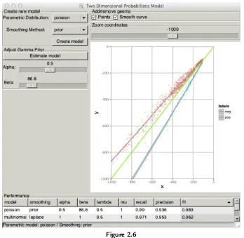
Chapter 2continues with a presentation of a visualization tool to assist in building Bayesian classifiers. The tool is developed using gWidgetsRGtk2 (Lawrence and Verzani, 2012) and ggplot2 (Wickham and Chang, 2012).
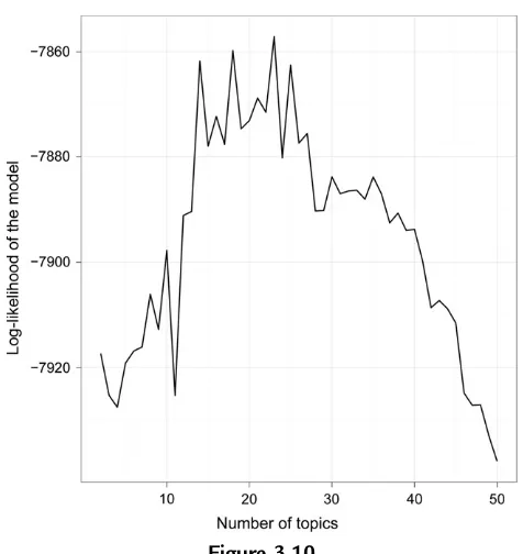
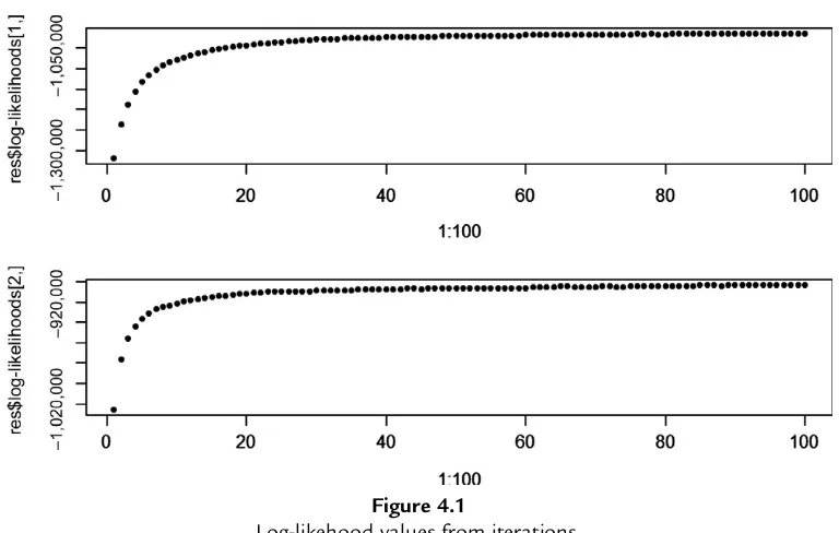
InChapters 3and4, we are given insights into the text mining capabilities of R. The twitteR package (Gentry, 2012) is used to source data for analysis inChapter 3. The data are
analyzed for emergent issues using the tm package (Feinerer and Hornik, 2012). The tm package is again used inChapter 4to analyze documents using latent Dirichlet allocation. As always there is ample R code to illustrate the different steps of collecting data, transforming the data, and analyzing the data.
InChapter 5, we move on to another larger area of application for data mining: recommender systems. The recommenderlab package (Hahsler, 2011) is extensively illustrated with practical examples. A number of different model builders are employed inChapter 6, looking at data mining in direct marketing. This theme of marketing and customer management is continued inChapter 7looking at the profiling of customers for insurance. A link to the dataset used is provided in order to make it easy to follow along.
Continuing with a business-orientation,Chapter 8discusses the critically important task of feature selection in the context of identifying customers who may default on their bank loans. Various R packages are used and a selection of visualizations provide insights into the data. Travelers and their preferences for hotels are analyzed inChapter 9 using Rfmtool.
Chapter 10begins a focus on some of the spatial and mapping capabilities of R for data mining. Spatial mapping and statistical analyses combine to provide insights into real estate pricing. Continuing with the spatial theme in data mining,Chapter 11deploys randomForest (Leo Breiman et al., 2012) for the prediction of the spatial distribution of seabed hardness. Chapter 12makes extensive use of the zooimage package (Grosjean and Francois, 2013) for image classification. For prediction, randomForest models are used, and throughout the chapter, we see the effective use of plots to illustrate the data and the modeling. The
Modeling many covariates inChapter 14to identify the most important ones takes us into the final chapters of the book. Italian football data, recording the outcome of matches, provide the basis for exploring a number of predictive model builders. Principal component analysis also plays a role in delivering the data mining project.
The book is rounded out with the application of data mining to the analysis of domain name system data. The aim is to deliver efficiencies for DNS servers. Cluster analysis using kmeans andkmedoids forms the primary tool, and the authors again make effective use of very many different types of visualizations.
The authors of all the chapters of this book provide and share a breadth of insights, illustrated through the use of R. There is much to learn by watching masters at work, and that is what we can gain from this book. Our focus should be on replicating the variety of analyses demonstrated throughout the book using our own data. There is so much we can learn about our own applications from doing so.
Graham Williams
February 20, 2013
References
R Core Team, 2012. R: a language and environment for statistical computing. R Foundation for Statistical Computing, Vienna, Austria. ISBN: 3-900051-07-0.http://www.R-project.org/.
Feinerer, I., Hornik, K., 2012. tm: Text Mining Package. R package version 0.5-8.1.http://CRAN.R-project.org/ package¼tm.
Gentry, J., 2012. twitteR: R based Twitter client. R package version 0.99.19.http://CRAN.R-project.org/ package¼twitteR.
Grosjean, P., Francois, K.D.R., 2013. zooimage: analysis of numerical zooplankton images. R package version 3.0-3.
http://CRAN.R-project.org/package¼zooimage.
Guha, S., 2012. Rhipe: R and Hadoop Integrated Programming Environment. R package version 0.69.http://www. rhipe.org/.
Hahsler, M., 2011. recommenderlab: lab for developing and testing recommender algorithms. R package version 0.1-3.http://CRAN.R-project.org/package¼recommenderlab.
Lawrence, M., Verzani, J., 2012. gWidgetsRGtk2: toolkit implementation of gWidgets for RGtk2. R package version 0.0-81.http://CRAN.R-project.org/package¼gWidgetsRGtk2.
Original by Leo Breiman, F., Cutler, A., port by Andy Liaw, R., Wiener, M., 2012. randomForest: Breiman and Cutler’s random forests for classification and regression. R package version 4.6-7.http://CRAN.R-project.org/ package¼randomForest.
Wickham, H., Chang, W., 2012. ggplot2: an implementation of the Grammar of Graphics. R package version 0.9.3.
http://had.co.nz/ggplot2/.
Power Grid Data Analysis with R
and Hadoop
Ryan Hafen, Tara Gibson, Kerstin Kleese van Dam, Terence Critchlow Pacific Northwest National Laboratory, Richland, Washington, USA
1.1 Introduction
This chapter presents an approach to analysis of large-scale time series sensor data collected from the electric power grid. This discussion is driven by our analysis of a real-world data set and, as such, does not provide a comprehensive exposition of either the tools used or the breadth of analysis appropriate for general time series data. Instead, we hope that this section provides the reader with sufficient information, motivation, and resources to address their own analysis challenges.
Our approach to data analysis is on the basis of exploratory data analysis techniques.
In particular, we perform an analysis over the entire data set to identify sequences of interest, use a small number of those sequences to develop an analysis algorithm that identifies the relevant pattern, and then run that algorithm over the entire data set to identify all instances of the target pattern. Our initial data set is a relatively modest 2TB data set, comprising just over 53 billion records generated from a distributed sensor network. Each record represents several sensor measurements at a specific location at a specific time. Sensors are geographically distributed but reside in a fixed, known location. Measurements are taken 30 times per second and synchronized using a global clock, enabling a precise reconstruction of events. Because all of the sensors are recording on the status of the same, tightly connected network, there should be a high correlation between all readings.
Given the size of our data set, simply running R on a desktop machine is not an option. To provide the required scalability, we use an analysis package called RHIPE (pronounced ree-pay) (RHIPE, 2012). RHIPE, short for the R and Hadoop Integrated Programming
Environment, provides an R interface to Hadoop. This interface hides much of the complexity of running parallel analyses, including many of the traditional Hadoop management tasks. Further, by providing access to all of the standard R functions, RHIPE allows the analyst to focus instead on the analysis of code development, even when exploring large data sets. A brief
Data Mining Applications with R #2014 Elsevier Inc. All rights reserved.
introduction to both the Hadoop programming paradigm, also known as the MapReduce paradigm, and RHIPE is provided inSection 1.3. We assume that readers already have a working knowledge of R.
As with many sensor data sets, there are a large number of erroneous records in the data, so a significant focus of our work has been on identifying and filtering these records. Identifying bad records requires a variety of analysis techniques including summary statistics, distribution checking, autocorrelation detection, and repeated value distribution characterization, all of which are discovered or verified by exploratory data analysis. Once the data set has been cleaned, meaningful events can be extracted. For example, events that result in a network partition or isolation of part of the network are extremely interesting to power engineers. The core of this chapter is the presentation of several example algorithms to manage, explore, clean, and apply basic feature extraction routines over our data set. These examples are generalized versions of the code we use in our analysis.Section 1.3.3.2.2describes these examples in detail, complete with sample code. Our hope is that this approach will provide the reader with a greater understanding of how to proceed when unique modifications to standard algorithms are warranted, which in our experience occurs quite frequently.
Before we dive into the analysis, however, we begin with an overview of the power grid, which is our application domain.
1.2 A Brief Overview of the Power Grid
The U.S. national power grid, also known as “the electrical grid” or simply “the grid,” was named the greatest engineering achievement of the twentieth century by the U.S. National Academy of Engineering (Wulf, 2000). Although many of us take for granted the flow of electricity when we flip a switch or plug in our chargers, it takes a large and complex infrastructure to reliably support our dependence on energy.
Built over 100 years ago, at its core the grid connects power producers and consumers through a complex network of transmission and distribution lines connecting almost every building in the country. Power producers use a variety of generator technologies, from coal to natural gas to nuclear and hydro, to create electricity. There are hundreds of large and small generation facilities spread across the country. Power is transferred from the generation facility to the transmission network, which moves it to where it is needed. The transmission network is comprised of high-voltage lines that connect the generators to distribution points. The network is designed with redundancy, which allows power to flow to most locations even when there is a break in the line or a generator goes down unexpectedly. At specific distribution points, the voltage is decreased and then transferred to the consumer. The distribution networks are disconnected from each other.
The US grid has been divided into three smaller grids: the western interconnection, the eastern interconnection, and the Texas interconnection. Although connections between these regions exist, there is limited ability to transfer power between them and thus each operates essentially as an independent power grid. It is interesting to note that the regions covered by these interconnections include parts of Canada and Mexico, highlighting our international
interdependency on reliable power. In order to be manageable, a single interconnect may be further broken down into regions which are much more tightly coupled than the major interconnects, but are operated independently.
Within each interconnect, there are several key roles that are required to ensure the smooth operation of the grid. In many cases, a single company will fill multiple roles—typically with policies in place to avoid a conflict of interest. The goal of the power producers is to produce power as cheaply as possible and sell it for as much as possible. Their responsibilities include maintaining the generation equipment and adjusting their generation based on guidance from a balancing authority. Thebalancing authorityis an independent agent responsible for ensuring the transmission network has sufficient power to meet demand, but not a significant excess. They will request power generators to adjust production on the basis of the real-time status of the entire network, taking into account not only demand, but factors such as transmission capacity on specific lines. They will also dynamically reconfigure the network, opening and closing switches, in response to these factors. Finally, the utility companies manage the distribution system, making sure that power is available to consumers. Within its distribution network, a utility may also dynamically reconfigure power flows in response to both planned and unplanned events. In addition to these primary roles, there are a variety of additional roles a company may play—for example, a company may lease the physical transmission or
distribution lines to another company which uses those to move power within its network. Significant communication between roles is required in order to ensure the stability of the grid, even in normal operating circumstances. In unusual circumstances, such as a major storm, communication becomes critical to responding to infrastructure damage in an effective and efficient manner.
Despite being over 100 years old, the grid remains remarkably stable and reliable.
operators. Further complicating the situation is the distribution of the renewable generators. Although some renewable sources, such as wind farms, share many properties with traditional generation capabilities—in particular, they generate significant amounts of power and are connected to the transmission system—consumer-based systems, such as solar panels on a business, are connected to the distribution network, not the transmission network. Although this distributed generation system can be extremely helpful at times, it is very different from the current model and introduces significant management complexity (e.g., it is not currently possible for a transmission operator to control when or how much power is being generated from solar panels on a house).
To address these needs, power companies are looking toward a number of technology solutions. One potential solution being considered is transitioning to real-time pricing of power. Today, the price of power is fixed for most customers—a watt used in the middle of the afternoon costs the same as a watt used in the middle of the night. However, the demand for power varies dramatically during the course of a day, with peak demand typically being during standard business hours. Under this scenario, the price for electricity would vary every few minutes depending on real-time demand. In theory, this would provide an incentive to minimize use during peak periods and transfer that utilization to other times. Because the grid infrastructure is designed to meet its peak load demands, excess capacity is available off-hours. By
redistributing demand, the overall amount of energy that could be delivered with the same infrastructure is increased. For this scenario to work, however, consumers must be willing to adjust their power utilization habits. In some cases, this can be done by making appliances cost aware and having consumers define how they want to respond to differences in price. For example, currently water heaters turn on and off solely on the basis of the water temperature in the tank—as soon as the temperature dips below a target temperature, the heater goes on. This happens without considering the time of day or water usage patterns by the consumer, which might indicate if the consumer even needs the water in the next few hours. A price-aware appliance could track usage patterns and delay heating the water until either the price of electricity fell below a certain limit or the water was expected to be needed soon. Similarly, an air conditioner might delay starting for 5 or 10 min to avoid using energy during a time of peak demand/high cost without the consumer even noticing.
Interestingly, the increasing popularity of plug-in electric cars provides both a challenge and a potential solution to the grid stability problems introduced by renewables. If the vehicles remain price insensitive, there is the potential for them to cause sudden, unexpected jumps in demand if a large number of them begin charging at the same time. For example, one car model comes from the factory preset to begin charging at midnight local time, with the expectation that this is a low-demand time. However, if there are hundreds or thousands of cars within a small area, all recharging at the same time, the sudden surge in demand becomes significant. If the cars are price aware, however, they can charge whenever demand is lowest, as long as they are fully charged when their owner is ready to go. This would spread out the charging over
the entire night, smoothing out the demand. In addition, a price-aware car could sell power to the grid at times of peak demand by partially draining its battery. This would benefit the owner through a buy low, sell high strategy and would mitigate the effect of short-term spikes in demand. This strategy could help stabilize the fluctuations caused by renewables by, essentially, providing a large-scale power storage capability.
In addition to making devices cost aware, the grid itself needs to undergo a significant change in order to support real-time pricing. In particular, the distribution system needs to be extended to support real-time recording of power consumption. Current power meters record overall consumption, but not when the consumption occurred. To enable this, many utilities are in the process of converting their customers tosmart meters. These new meters are capable of sending the utility real-time consumption information and have other advantages, such as dramatically reducing the time required to read the meters, which have encouraged their adoption. On the transmission side, existing sensors provide operators with the status of the grid every 4 seconds. This is not expected to be sufficient given increasing variability, and thus new sensors called phasor measurement units (PMUs) are being deployed. PMUs provide information 30-60 times per second. The sensors are time synchronized to a global clock so that the state of the grid at a specific time can be accurately reconstructed. Currently, only a few hundred PMUs are deployed; however, the NASPI project anticipates having over 1000 PMUs online by the end of 2014 (Silverstein, 2012) with a final goal of between 10,000 and 50,000 sensors deployed over the next 20 years. An important side effect of the new sensors on the transmission and distribution networks is a significant increase in the amount of information that power companies need to collect and process. Currently, companies are using the real-time streams to identify some critical events, but are not effectively analyzing the resulting data set. The reasons for this are twofold. First, the algorithms that have been developed in the past are not scaling to these new data sets. Second, exactly what new insights can be gleaned from this more refined data is not clear. Developing scalable algorithms for known events is clearly a first step. However, additional investigation into the data set using techniques such as exploratory analysis is required to fully utilize this new source of information.
1.3 Introduction to MapReduce, Hadoop, and RHIPE
Before presenting the power grid data analysis, we first provide an overview of MapReduce and associated topics including Hadoop and RHIPE. We present and discuss the implementation of a simple MapReduce example using RHIPE. Finally, we discuss other parallel R approaches for dealing with large-scale data analysis. The goal is to provide enough background for the reader to be comfortable with the examples provided in the following section.
description of MapReduce through a concrete example, introduce basic RHIPE commands, and prepare the reader to follow the code examples on our power grid work presented in the following section. In the interest of space, our explanations focus on the various aspects of RHIPE, and not on R itself. A reasonable skill level of R programming is assumed.
A lengthy exposition on all of the facets of RHIPE is not provided. For more details, including information about installation, job monitoring, configuration, debugging, and some advanced options, we refer the reader toRHIPE (2012)andWhite (2010).
1.3.1 MapReduce
MapReduce is a simple but powerful programming model for breaking a task into pieces and operating on those pieces in an embarrassingly parallel manner across a cluster. The approach was popularized by Google (Dean and Ghemawat, 2008) and is in wide use by companies processing massive amounts of data.
MapReduce algorithms operate on data structures represented askey/valuepairs. The data are split into blocks; each block is represented as a key and value. Typically, the key is a descriptive data structure of the data in the block, whereas the value is the actual data for the block. MapReduce methods perform independent parallel operations on input key/value pairs and their output is also key/value pairs. The MapReduce model is comprised of two phases, themap
and thereduce, which work as follows:
Map: A map function is applied to each input key/value pair, which does some user-defined processing and emits new key/value pairs to intermediate storage to be processed by the reduce.
Shuffle/Sort: The map output values are collected for each unique map output key and passed to a reduce function.
Reduce: A reduce function is applied in parallel to all values corresponding to each unique map output key and emits output key/value pairs.
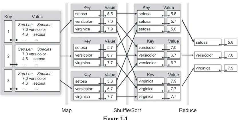
1.3.1.1 An Example: The Iris Data
The iris data are very small and methods can be applied to it in memory, within R, without splitting it into pieces and applying MapReduce algorithms. It is an accessible introductory example nonetheless, as it is easy to verify computations done with MapReduce to those with the traditional approach. It is the MapReduce principles—not the size of the data—that are important: Once an algorithm has been expressed in MapReduce terms, it theoretically can be applied unchanged to much larger data.
The iris data are a data frame of 150 measurements of iris petal and sepal lengths and widths, with 50 measurements for each species of “setosa,” “versicolor,” and “virginica.” Let us assume that we are doing some computation on the sepal length. To simulate the notion of data
being partitioned and distributed, consider the data being randomly split into 3 blocks. We can achieve this in R with the following:
>set.seed(4321) # make sure that we always get the same partition >permute<- sample(1:150, 150)
>splits<- rep(1:3, 50)
>irisSplit<- tapply(permute, splits, function(x) { iris[x, c(“Sepal.Length”, “Species”)]
})
>irisSplit $‘1’
Sepal.Length Species
51 7.0 versicolor
7 4.6 setosa
. . .# output truncated
Throughout this chapter, code blocks that also display output will distinguish lines containing code with “>” at the beginning of the line. Code blocks that do not display output do not add this distinction.
This partitions theSepal.LengthandSpeciesvariables into three random subsets, having the keys “1,” “2,” or “3,” which correspond to our blocks. Consider a calculation of the maximum sepal length by species withirisSplitas the set of input key/value pairs. This can be achieved with MapReduce by the following steps:
Map: Apply a function to each division of the data which, for each species, computes the maximum sepal length and outputs key¼species and value¼max sepal length.
Shuffle/Sort: Gather all map outputs with key “setosa” and send to one reduce, then all with key “versicolor” to another reduce, etc.
Reduce: Apply a function to all values corresponding to each unique map output key (species) which gathers and calculates the maximum of the values.
It can be helpful to view this process visually, as is shown inFigure 1.1. The input data are theirisSplit set of key/value pairs. As described in the steps above, applying the map to each input key/value pair emits a key/value pair of the maximum sepal length per species. These are gathered by key (species) and the reduce step is applied which
calculates a maximum of maximums, finally outputting a maximum sepal length per species. We will revisit this Figure with a more detailed explanation of the calculation in
Section 1.3.3.2.
1.3.2 Hadoop
Hadoop is an open-source distributed software system for writing MapReduce
System (HDFS) and the MapReduce parallel compute engine. Hadoop was inspired by papers written about Google’s MapReduce and Google File System (Dean and Ghemawat, 2008). Hadoop handles data by distributing key/value pairs into the HDFS. Hadoop schedules and executes the computations on the key/value pairs in parallel, attempting to minimize data movement. Hadoop handles load balancing and automatically restarts jobs when a fault is encountered. Hadoop has changed the way many organizations work with their data, bringing cluster computing to people with little knowledge of the complexities of distributed programming. Once an algorithm has been written the “MapReduce way,” Hadoop provides concurrency, scalability, and reliability for free.
1.3.3 RHIPE: R with Hadoop
RHIPE is a merger of R and Hadoop. It enables an analyst of large data to apply numeric or visualization methods in R. Integration of R and Hadoop is accomplished by a set of components written in R and Java. The components handle the passing of information between R and Hadoop, making the internals of Hadoop transparent to the user. However, the user must be aware of MapReduce as well as parameters for tuning the performance of a Hadoop job. One of the main advantages of using R with Hadoop is that it allows rapid prototyping of methods and algorithms. Although R is not as fast as pure Java, it was designed as a
programming environment for working with data and has a wealth of statistical methods and tools for data analysis and manipulation.
Reduce
An Illustration of applying a MapReduce job to calculate the maximum Sepal. Length by Species for the irisSplit data.
1.3.3.1 Installation
RHIPE depends on Hadoop, which can be tricky to install and set up. Excellent references for setting up Hadoop can be found on the web. The site www.rhipe.org provides installation instructions for RHIPE as well as a virtual machine with a local single-node Hadoop cluster. A single-node setup is good for experimenting with RHIPE syntax and for prototyping jobs before attempting to run at scale. Whereas we used a large institutional cluster to perform analyses on our real data, all examples in this chapter were run on a single-node virtual machine. We are using RHIPE version 0.72. Although RHIPE is a mature project, software can change over time. We advise the reader to checkwww.rhipe.orgfor notes of any changes since version 0.72.
Once RHIPE is installed, it can be loaded into your R session as follows:
>library(Rhipe)
---| IMPORTANT: Before using Rhipe call rhinit() | | Rhipe will not work or most probably crash | --->rhinit()
Rhipe initialization complete Rhipe first run complete Initializing mapfile caches [1] TRUE
>hdfs.setwd(“/”)
RHIPE initialization starts a JVM on the local machine that communicates with the cluster. The
hdfs.setwd()command is similar to R’ssetwd()in that it specifies the base directory to which all references to files on HDFS will be subsequently based on.
1.3.3.2 Iris MapReduce Example with RHIPE
To execute the example described inSection 1.3.1.1, we first need to modify theirisSplit
data to have the key/value pair structure that RHIPE expects. Key/value pairs in RHIPE are represented as an R list, where each list element is another list of two elements, the first being a key and the second being the associated value. Keys and values can be arbitrary R objects. The list of key-value pairs is written to HDFS using rhwrite ():
>irisSplit<- lapply(seq_along(irisSplit), function(i) þlist(i, irisSplit[[i]])
þ)
>rhwrite(irisSplit, “irisData”) Wrote 3 pairs occupying 2100 bytes
directory, but since this data set is so small, it only requires one file. This file can now serve as an input to RHIPE MapReduce jobs.
1.3.3.2.1 The Map Expression
Below is a map expression for the MapReduce task of computing the maximum sepal length by species. This expression transforms the random data splits in the irisData file into a partial answer by computing the maximum of each species within each of the three splits. This significantly reduces the amount of information passed to the shuffle sort, since there will be three sets (one for each of the map keys) of at most three key-value pairs (one for each species in each map value).
maxMap<- expression({ for(r in map.values) {
by(r, r$Species, function(x) { rhcollect(
as.character(x$Species[1]), # key max(x$Sepal.Length) # value )
}) } })
RHIPE initializes themap.values object to be an R list with the input keys and values for each map task to process. Typically, multiple map expressions are executed in parallel with batches of key/value pairs being passed in until all key/value pairs have been processed. Hadoop takes care of the task distribution, relaunching map tasks when failures occur and attempting to keep the computation local to the data. Because each map task operates on only the subset of the keys and values, it is important that they do not make improper assumptions about which data elements are being processed.
The above map expression cycles through the input key/value pairs for eachmap.value, calculating the maximum sepal length by species for each of the data partitions. The function
rhcollect()emits key/value pairs to be shuffled and sorted before being passed to the reduce expression. The map expression generates three output collections, one for each of the unique keys output by the map, which is the species. Each collection contains three elements corresponding to the maximum sepal length for that species found within the associated map value. This is visually depicted by the Map step inFigure 1.1. In this example, the inputmap.keys(“1,” “2,” and “3”) are not used since they are not meaningful for the computation.
Debugging expressions in parallel can be extremely challenging. As a validation step, it can be useful for checking code correctness to step through the map expression code manually (up torhcollect(), which only works inside of a real RHIPE job), on a single processor and with a small data set, to ensure that it works as expected. Sample inputmap.keysandmap. valuescan be obtained by extracting them fromirisSplit:
Then one can proceed through the map expression to investigate what the code is doing.
1.3.3.2.2 The Reduce Expression
Hadoop automatically performs the shuffle/sort step after the map task has been executed, gathering all values with the same map output key and passing them to the same reduce task. Similar to the map step, the reduce expression is passed key/value pairs through thereduce. keyand associatedreduce.values. Because the shuffle/sort combines values with the same key, each reduce task can assume that it will process all values for a given key (unlike the map task). Nonetheless, because the number of values can be large, thereduce.valuesare fed into the reduce expression in batches.
maxReduce<- expression( pre¼{
speciesMax<- NULL },
reduce¼{
speciesMax<- max(c(speciesMax, do.call(c, reduce.values))) },
post¼{
rhcollect(reduce.key, speciesMax) }
)
To manage the sequence of values, the reduce expression is actually defined as a vector of expressions,pre, reduce, andpost. Thepreexpression is executed once at the beginning of the reduce phase for eachreduce.key value. The reduce expression is executed each time newreduce.valuesarrive, and thepostexpression is executed after all values have been processed for the particularreduce.key. In our example, pre is used to initialize the
speciesMaxvalue toNULL. Thereduce.valuesarrive as a list of a collection of the emitted map values, which for this example is a list of scalars corresponding to the sepal lengths. We updatespeciesMax by calculating the maximum of thereduce.valuesand the current value ofspeciesMax. For a given reduce key, the reduceexpression may be invoked multiple times, each time with a new batch ofreduce.values, and updating in this manner assures us that we ultimately obtain the maximum of all maximums for the given species. The
postexpression is used to generate the final key/value pairs from this execution, each species and its maximum sepal length.
1.3.3.2.3 Running the Job
RHIPE jobs are prepared and run using therhwatch()command, which at a minimum requires the specification of the map and reduce expressions and the input and output directories.
>maxSepalLength<- rhwatch( þmap¼maxMap,
þreduce¼maxReduce, þinput¼"irisData",
þ)
. . .
job_201301212335_0001, State: PREP, Duration: 5.112
URL:http://localhost:50030/jobdetails.jsp?jobid¼job_201301212335_0001 pct numtasks pending running complete killed failed_attempts
map 0 1 1 0 0 0 0
reduce 0 1 1 0 0 0 0
killed_attempts
map 0
reduce 0
Waiting 5 seconds
. . .
Note that the time it takes this job to execute (30 s) is longer than it would take to do the simple calculation in memory in R. There is a small overhead with launching a RHIPE MapReduce job that becomes negligible as the size of the data grows.
rhwatch()specifies, at a minimum, the map and reduce expressions and the input and output directories. There are many more options that can be specified here, including Hadoop parameters. Choosing the right Hadoop parameters varies by the data, the algorithm, and the cluster setup, and is beyond the scope of this chapter. We direct the interested reader to the
rhwatch()help page and to (White, 2010) for appropriate guides on Hadoop parameter selection. All examples provided in the chapter should run without problems on the virtual machine available atwww.rhipe.orgusing the default parameter settings.
Some of the printed output of the call torhwatch()is truncated in the interest of space. The printed output basically provides information about the status of the job. Above, we see output from the setup phase of the job. There is one map task and one reduce task. With larger data and on a larger cluster, the number of tasks will be different, and mainly depend on Hadoop parameters which can be set through RHIPE or in the Hadoop configuration files. Hadoop has a web-based job monitoring tool whose URL is specified when the job is launched, and the URL to this is supplied in the printed output.
The output of the MapReduce job is stored by default as a Hadoop sequence file of key/value pairs on HDFS in the directory specified byoutput(here, it isirisMaxSepalLength. By default,rhwatch()reads these data in after job completion and returns it. If the output of the job is too large, as is often the case, and we don’t want to immediately read it back in but instead use it for subsequent MapReduce jobs, we can addreadback¼FALSEto ourrhwatch()call and then later on callrhread(“irisMaxSepalLength”). In this chapter, we will usually read back results in the examples since the output datasets are small.
1.3.3.2.4 Looking at Results
The output from a MapReduce run is the set of key/value pairs generated by the reduce expression. In exploratory data analysis, often it is important to reduce the data to a size that is manageable within a single, local R session. Typically, this is accomplished by iterative
applications of MapReduce to transform, subset, or reduce the data. In this example, the result is simply a list of three key-value pairs.
>maxSepalLength [[1]]
[[1]][[1]] [1] “setosa” [[1]][[2]] [1] 5.8
. . .
>do.call("rbind", lapply(maxSepalLength, function(x) { þ data.frame(species¼x[[1]], max¼x[[2]])
þ}))
species max 1 setosa 5.8 2 virginica 7.9 3 versicolor 7.0
We see that maxSepalLength is a list of key/value pairs. This code turns this list of key/value pairs into a more suitable format, extracting the key (species) and maximum for each pair and binding them into adata.frame.
Before moving on, we introduce a simplified way to create map expressions. Typically, a RHIPE map expression as defined above for the iris example simply iterates over groups of key/value pairs provided asmap.keysandmap.valueslists. To avoid this repetition, a wrapper function,
rhmap()has been created, that is applied to each element ofmap.keysandmap.values, where the currentmap.keyselement is available as m, and the currentmap.valueselement is available as r. Thus, the map expression for the iris example could be rewritten as
maxMap<- rhmap({
by(r, r$Species, function(x) { rhcollect(
as.character(x$Species[1]), # key max(x$Sepal.Length) # value )
}) })
This simplification will be used in all subsequent examples.
1.3.4 Other Parallel R Packages
As evidenced by over 4000 R add-on packages available on the Comprehensive R Archive Network (CRAN), there are many ways to get things done in R. Parallel processing is no exception. High-performance computing with R is very dynamic, and a good place to find up-to-date information about what is available is the CRAN task view for high-performance computing.1Nevertheless, this chapter would not be complete without a brief overview of some
1
other parallel packages available at this time. The interested reader is directed to a very good, in-depth discussion about standard parallel R approaches in (McCallum and Weston, 2011). There are a number of R packages for parallel computation that are not suited for analysis of large amounts of data. Two of the most popular parallel packages are snow (Tierney et al., 2012) and multicore (Urbanek, 2011), versions of which are now part of the base R package
parallel(R Core Team, 2012). These packages enable embarrassingly parallel computation on multiple cores and are excellent for CPU heavy tasks. Unfortunately, it is incumbent upon the analyst to define how each process interacts with the data and how the data are stored. Using the MapReduce paradigm with these packages is tedious because the user must explicitly perform the intermediate storage and shuffle/sort tasks, which Hadoop takes care of automatically. Finally, these packages do not provide automatic fault tolerance, which is extremely important when computations are spread out over hundreds or thousands of cores. R packages that allow for dealing with larger data outside of R’s memory includeff(Adler et al., 2012), bigmemory (Kane and Emerson, 2011), and RevoScaleR (Revolution Analytics, 2012a,b). These packages have specialized formats to store matrices or data frames with a very large number of rows. They have corresponding packages that perform
computation of several standard statistical methods on these data objects, much of which can be done in parallel. We do not have extensive experience with these packages, but we presume that they work very well for moderate-sized, well-structured data. When the data must be spread across multiple machines and is possibly unstructured, however, we turn to solutions like Hadoop.
There are multiple approaches for using Hadoop with R. Hadoop Streaming, a part of Hadoop that allows any executable, which reads from standard input and writes to standard output to be used as map and reduce processes, can be used to process R executables. The rmr package (Revolution Analytics, 2012a,b) builds upon this capability to simplify the process of creating the map and reducing tasks. RHIPE and rmr are similar in what they accomplish: using R with Hadoop without leaving the R console. The major difference is that RHIPE is integrated with Hadoop’s Java API whereas rmr uses Hadoop Streaming. The rmr package is a good choice for a user satisfied with the Hadoop Streaming interface. RHIPE’s design around the Java API allows for a more managed interaction with Hadoop during the analysis process. Thesegue
package (Long, 2012) allows forlapply()style computation using Hadoop on Amazon Elastic MapReduce. It is very simple, but limited for general-purpose computing.
1.4 Power Grid Analytical Approach
This section presents both a synopsis of the methodologies we applied to our 2TB power grid data set and details about their implementation. These methodologies include aspects of exploratory analysis, data cleaning, and event detection. Some of the methods are
straightforward and could be accomplished using a variety of techniques, whereas others clearly exhibit the power and simplicity of MapReduce. Although this approach is not suited for every data mining problem, the following examples should demonstrate that it does provide a powerful and scalable rapid development environment for a breadth of data mining tasks.
1.4.1 Data Preparation
Preprocessing data into suitable formats is an important consideration for any analysis task, but particularly so when using MapReduce. In particular, the data must be partitioned into key/ value pairs in a way that makes the resulting analysis efficient. This applies to both optionally reformatting the original data into a format that can be manipulated by R and partitioning the data in a way that supports the required analyses. In general, it is not uncommon to partition the data along multiple dimensions to support different analyses.
As a first step, it is worthwhile to convert the raw data into a format that can be quickly ingested by R. For example, converting data from a customized binary file into an R data frame dramatically reduces read times for subsequent analyses. The raw PMU data were provided in a proprietary binary format that uses files to partition the data. Each file contains approximately 9000 records, representing 5 min of data. Each record contains 555 variables representing the time and multiple measurements for each sensor.
We provide R code inAppendixto generate a synthetic data set of frequency measurements and flags, a subset of 76 variables out of the 555. These synthetic data are a simplified version of the actual PMU data, containing only the information required to execute the examples in this section. Where appropriate, we motivate our analysis using results pulled from the actual data set. The attentive reader will notice that these results will typically not exhibit the same properties as the same analysis performed on the synthetic data, although we tried to artificially preserve some of these properties. Although unfortunate, that difference is to be expected. The major consideration when partitioning the data is determining how to best split it into key/ value pairs. Our analyses are primarily focused on time-local behavior, and therefore the original partitioning of the data into 5-min time intervals is maintained. Five minutes is an appropriate size for analysis because interesting time-local behaviors occur in intervals spanning only a few seconds, and the blocks are of an adequate size (11 MB per serialized block) for multiple blocks to be read in to the map function at a given time. However, many raw data files do not contain exactly 5 min of data, so some additional preprocessing is required to fill in missing information. For simplicity, the synthetic data set comprises 10 complete 5-min partitions.
1.4.2 Exploratory Analysis and Data Cleaning
A good first step in the data mining process is to visually and numerically explore the data. With large data sets, this is often initially accomplished through summaries
since a direct analysis of the detailed records can be overwhelming. Although summaries can mask interesting features of the full data, they can also provide immediate insights. Once the data are understood at the high level, analysis of the detailed records can be fruitful.
1.4.2.1 5-min Summaries
A simple summary of frequency over a 5-min window for each PMU provides a good starting point for understanding the data. This calculation is straightforward: since the data are already divided into 5-min blocks the computation simply calculates summary statistics at each time stamp split by PMU. The map expression for this task is:
map.pmusumm<- rhmap({
# r is the data.frame of values for a 5-minute block # k is the key (time) for the block
colNames<- colnames(r)
freqColumns<- which(grepl(“freq”, colNames))
pmuName<- gsub(“(.*)\\.freq”, “\\1”, colNames[freqColumns]) for(j in seq_along(freqColumns)) { # loop through frequency columns
v<- r[,freqColumns[j]] / 1000þ60 # convert to HZ rhcollect(
pmuName[j], # key is the PMU data.frame(
time ¼k,
min ¼min( v, na.rm¼TRUE), max ¼max( v, na.rm¼TRUE), mean ¼mean( v, na.rm¼TRUE), stdev ¼sd( v, na.rm¼TRUE), median¼median(v, na.rm¼TRUE), nna ¼length(which(is.na(v))) )
) } })
The first three lines after the comments extract only the PMU frequency columns (because the data frame consists of column names ending with “.freq” and “.flag”). These three lines will be recycled in most of the subsequent examples. These columns are then iterated over, converting the 1000 offset from 60 HZ to a true frequency value and calculating a data frame of summary statistics which is emitted to the reduce function with the PMU as the key. This map task emits 38 key/value pairs (one for each PMU) for each input key (time interval).
The reduce collects all of the values for each unique PMU and collates them:
reduce.pmusumm<- expression( pre¼{
res<- NULL },
reduce¼{
res<- do.call(rbind, c(list(res), reduce.values)) },
post¼{
res<- res[order(res$time),] # order results by time
res$time<- as.POSIXct(res$time, origin¼"1970-01-01", tz¼"UTC") rhcollect(reduce.key, res)
} )
Recall that the reduce expression is applied to each collection of unique map output keys, which in this case is the PMU identifier. Thepreexpression is evaluated once for each key, initializing the result data frame. Thereduceexpression is evaluated as newreduce.values
flow in iteratively building the data frame. Finally, thepostexpression orders the result by time, converts the time to an RPOSIXct object, and writes the result.
We run the job by:
summ5min<- rhwatch( map¼map.pmusumm, reduce¼reduce.pmusumm, input¼“blocks5min”,
output¼"blocks5min_summary” )
To look at the first key/value pair:
>summ5min[[1]][[1]] [1] “AA”
>str(summ5min[[1]][[2]])
‘data.frame’: 10 obs. of 7 variables:
$ time : POSIXct, format: “2012-01-01 00:00:00” “2012-01-01 00:05:00” “2012-01-01 00:10:00”
. . .
$ min : num 60 60 60 60 60. . .
$ max : num 60 60 60 60 60. . .
$ mean : num 60 60 60 60 60. . .
$ stdev : num 0.00274 0.00313 0.0044 0.0028 0.00391. . .
$ median: num 60 60 60 60 60. . .
$ nna : int 0 0 0 0 0 0 0 0 0 0
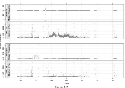
interval.Figure 1.2 shows a plot of 5-min median frequencies and number of missing observations across time for two PMUs as calculated from the real data.
Plots like these helped identify regions of data for which the median frequency was so out-of-bounds that it could not be trusted.
1.4.2.2 Quantile Plots of Frequency
A summary that provides information about the distribution of the frequency values for each PMU is a quantile plot. Calculating exact quantiles would require collecting all of the frequency values for each PMU, about 1.4 billion values, then applying a quantile algorithm. This is an example where a simplified algorithm that achieves an approximate solution is very useful. An approximate quantile plot can be achieved by first discretizing the data through rounding and then tabulating the unique values. Great care must be taken in choosing how to discretize the data to ensure that the resulting distribution is not oversimplified. The PMU frequency data are already discretely reported as an integer 1000 offset from 60 HZ. Thus, our task is to tabulate the unique frequency values by PMU and translate the tabulation into quantiles. Here, as in the previous
Figure 1.2
5-min medians and number of missing values versus time for two PMUs.
example, we are transforming data split by time to data split by PMU. This time, we are aggregating across time as well, tabulating the occurrence of each unique frequency value:
map.freqquant<- rhmap({ colNames<- colnames(r)
freqColumns<- which(grepl("freq", colNames))
pmuName<- gsub("(.*)\\.freq", “\\1", colNames[freqColumns]) for(j in seq_along(freqColumns)) { # loop through frequency columns
freqtab<- table(r[,freqColumns[j]]) rhcollect(
pmuName[j], # key is the PMU data.frame(
level¼as.integer(names(freqtab)), count¼as.numeric(freqtab)
) ) } })
As a result, this map task is similar to that of the previous example. The only difference is the data frame of tabulated counts of frequencies that is being passed to the reduce expression.2The map expression emits one data frame of tabulations for each PMU for each time block. The reduce function must combine a collection of tabulations for a given PMU:
reduce.tab<- expression( pre¼{
res<- NULL },
reduce¼{
tabUpdate<- do.call(rbind, c(list(res), reduce.values)) tabUpdate<- xtabs(countlevel, data¼tabUpdate) res<- data.frame(
level¼as.integer(names(tabUpdate)), count¼as.numeric(tabUpdate)
) }, post¼{
rhcollect(reduce.key, res) }
)
For each PMU, we combine the data frames of the tabulation output and create a new tabulation data frame using R’sxtabs()function. This function sums the already-computed counts instead of simply counting the number of unique occurrences. The call toas.numeric()is required because the count may become too large to be represented as an integer. As is common
2
in reduce steps, the output of thereduceexpression is of the same format as the values emitted from the map, allowing it to be easily updated as newreduce.valuesarrive. This function is a generalized reduce that can be applied to other computations.
To execute the job:
freqtab<- rhwatch(
map¼map.freqquant, reduce¼reduce.tab,
input¼"blocks5min", output¼"frequency_quantile” )
The data and computed quantiles for the first PMU can be manipulated and viewed by:
ftpmu<- freqtab[[1]][[2]] cs<- cumsum(ftpmu$count) f<- ppoints(2000, 1)
q<- ftpmu$level[sapply(f * sum(ftpmu$count), function(x) min(which(x<¼cs)))]
plot(f, q / 1000þ60, xlab¼"Quantile", ylab¼"Frequency (HZ)")
Here,csis the cumulative sum of the tabulated frequencies, andfis the vector of discrete values which had been recorded by the PMU. The quantile,q[i], for a given value off[i]is the value at which the number of counts corresponding to f[i] is less than or equal to the cumulative sum. This code essentially turns our frequency tabulation into
approximate quantiles.
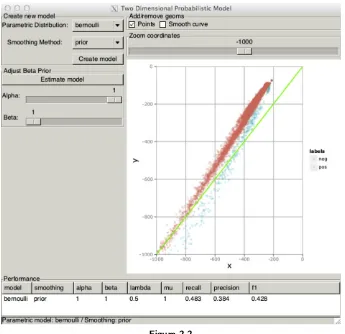
The distribution of frequency for many of the PMUs was approximately normal.Figure 1.3
shows normal-quantile plots for two PMUs in the real data set. The distribution of frequency for PMU A looks approximately normal, whereas that for PMU B has an abnormally high amount of frequency values right below 60 HZ. This indicates data integrity issues.
As implied by the previous two examples, there are many observations in this data set that are suspect. With RHIPE, we can perform calculations across the entire data set to uncover and confirm the bad data cases while developing algorithms for removing these cases from the data. A conservative approach filters only impossible data values, ensuring that anomalous data are not unintentionally filtered out by these algorithms. Furthermore, the original data set is unchanged by the filters, which are applied on demand to remove specific types of information from the data set.
1.4.2.3 Tabulating Frequency by Flag
Investigating the strange behavior of the quantile plots required looking at other aspects of the data including the PMU flag. The initial information from one expert was that flag 128 is a signal for bad data. Our first step was to verify this and then gain insight into the other flags. Tabulating frequency by PMU and flag can indicate whether or not the frequency behaves differently based on the flag settings. This involves a computation similar to the quantile calculation, except that we step through each unique flag for each PMU, and emit a vector with
the current PMU and flag for which frequencies are being tabulated. For the sake of brevity, we omit the code for this example but encourage the reader to implement this task on the synthetic data provided.
When applying this to the real data, we found that for any flag greater than or equal to 128, the frequency is virtually always set at 1 (59.999 HZ). This insight, combined with visual confirmation that the values did not appear to be plausible, implied that these flags are indicative of bad data. This was later confirmed by another expert.
1.4.2.4 Distribution of Repeated Values
Even after filtering the additional bad data flags, the quantile plots indicated some values that occurred more frequently than expected. Investigating the frequency plots further, we identified some cases where extended sequences of repeated frequency values occurred. This was quantified by calculating the distribution of the sequence length of repeated values. The sequence length distribution is calculated by stepping through a 5-min block of data and, for each PMU and given frequency valuex, finding all runs ofxand counting the run length. Then the number of times each run length occurs is tabulated. This can be achieved with:
map.repeat<- rhmap({ colNames<- colnames(r)
Figure 1.3
freqColumns<- which(grepl("freq", colNames))
pmuName<- gsub("(.*)\\.freq", “\\1", colNames[freqColumns]) for(j in seq_along(freqColumns)) { # step through frequency columns
curFreq<- r[,freqColumns[j]]
curFreq<- curFreq[!is.na(curFreq)] # omit missing values changeIndex<- which(diff(curFreq) !¼0) # find index of changes changeIndex<- c(0, changeIndex, length(curFreq)) # pad with beg/end runLengths<- diff(changeIndex) # run length is diff between changes runValues<- curFreq[changeIndex[-1]] # get value assoc with lengths uRunValues<- unique(runValues)
for(val in uRunValues) { # for each unique runValue tabulate lengths repeatTab<- table(runLengths[runValues¼¼val])
rhcollect(
list(pmuName[j], val), data.frame(
level¼as.integer(names(repeatTab)), count¼as.numeric(repeatTab)
) ) } } })
curFreqis the current frequency time series for which we are tabulating runs, with missing values omitted. We find all places wherecurFreqchanges from one number to another by finding where all first differences are not zero, storing the result aschangeIndex. We calculaterunLengthsby taking the first difference ofchangeIndex. Then, for each uniquerunValue, we tabulate the count of each sequence length and pass it to the reduce.
Because this tabulation in the map occurs on a single 5-min window, the largest possible sequence length is 9000 (5 min * 30 records/s). For our purposes, this is acceptable because we are looking for impossibly long sequences of values, and a value repeating for even 1 min or more is impossibly long. We do not need to accurately count the length of every run; we only identify those repetitions that are too long to occur in a correctly working system. Further, if a sequence happens to slip by the filter, for example, because it is equally split across files, there is little harm done. An exact calculation could be made, but the additional algorithmic complexity is not worthwhile in our case.
Since we emit data frames of the same format as those expected byreduce.tab(Section 1.4), we simply define it as our reduce function. This reuse is enabled because we precede the tabulation with a nontrivial transformation of the data to sequence lengths. As previously noted, many map algorithms can be defined to generate input to this function. The job is executed by:
repeatTab<- rhwatch(
map¼map.repeat, reduce¼reduce.tab,
input¼"blocks5min", output¼"frequency_repeated” )
And we can visualize the results for repeated 60 HZ frequencies by:
repeatZero<- do.call(rbind, lapply(repeatTab, function(x) { if(x[[1]][[2]]¼¼0) {
data.frame(pmu¼x[[1]][[1]], x[[2]]) }
}))
library(lattice)
xyplot(log2(count)log2(level) | pmu, data¼repeatZero)
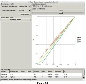
The lattice package plots the distribution of repeated 60H values by PMU, shown for two PMUs inFigure 1.4 for the real PMU data.
Figure 1.4 shows this plot for real PMUs on a log-log scale. The solid black line indicates the tail of a geometric probability distribution fit to the tail of the repeated value distribution. We can use this observation to set limits based on the estimated geometric parameters which we would likely never expect to see a run length exceed. PMU AS inFigure 1.4
shows several cases well beyond the tail of a legitimate distribution. These sequences of well over 45 s correspond to bad data records. An interesting side effect of this analysis was that domain experts were quite surprised that sequence lengths as long as 3 seconds are not only completely plausible according to the distribution—but actually occur frequently in practice.
1.4.2.5 White Noise
A final type of bad sensor data occurs when the data have a high degree of randomness. Because the sensors model a physical system, with real limitations on how fast state can change, a high degree of autocorrelation in frequency is expected. When data values are essentially random, the sensor is clearly not operating correctly and the values should be
Figure 1.4
discarded—even when they fall within a normal range. We call this effect “white noise.” The first column inFigure 1.5shows two PMUs with a normal frequency distribution and a third producing white noise.
One way to detect this behavior is to apply the Ljung-Box test statistic to each block of data. This determines whether any of a group of autocorrelations is significantly different from zero. As seen in the second column ofFigure 1.5, the autocorrelation function for the regular frequency series trails off very slowly, whereas it quickly decreases for the final PMU indicating a lack of correlation. Applying this test to the data identifies local regions where this behavior is occurring.
This is relatively straightforward to implement:
map.ljung<- rhmap({ colNames<- colnames(r)
freqColumns<- which(grepl(“freq”, colNames))
pmuName<- gsub(“(.*)\\.freq”, “\\1”, colNames[freqColumns]) # apply Box.test() to each column
pvalues<- apply(r[,freqColumns], 2, function(x) { boxres<- try(
Figure 1.5
Time series (left) and sample autocorrelation function (right) for three real PMU 5-min frequency series.
Box.test(x, lag¼10, type¼“Ljung-Box”)$p.value, silent¼TRUE
)
ifelse(inherits(boxres, “try-error”), NA, boxres) })
rhcollect( “1”,
data.frame(time¼k, t(pvalues)) )
})
This map uses the built-in R function,Box.test() andbuilds the result across allmap. valuesbefore callingrhcollect().It also provides an example of handling R errors by checking to see if theBox.test()call produced an error. If RHIPE detects R errors, the job will not be completed so it is important this error is caught and handled by the map function. The map output key in all cases is simply “1,” which is an arbitrary choice which ensures all map outputs go to the same reduce.
The reduce collates theP-values and usesreduce.rbindto convert them into a single data frame ofP-values.
reduce.rbind<- expression( pre¼{
res<- NULL },
reduce¼{
res<- rbind(res, do.call(rbind, reduce.values)) },
post¼{
rhcollect(reduce.key, res) }
)
ljungPval<- rhwatch(
map¼map.ljung, reduce¼reduce.rbind,
input¼“blocks5min”, output¼“frequency_ljung” )
We can now search for PMUs and time intervals with nonsignificantP-values. For the simulated data, we see that the results show the detection of the white noise that was inserted into theAA.freq series at the 10th time step.
1.4.3 Event Extraction