EXPLORING CLIMATE CHANGE EFFECTS ON WATERSHED SEDIMENT YIELD
AND LAND COVER-BASED MITIGATION MEASURES USING SWAT MODEL, RS
AND GIS: CASE OF CAGAYAN RIVER BASIN, PHILIPPINES
Jeark A. Principe
Graduate student, Department of Geodetic Engineering, University of the Philippines Diliman, Melchor Hall, College of Engineering, U.P. Diliman, Quezon City, Philippines;
Tel: +63-02-9818500 loc. 3124; E-mail: jeark_principe@yahoo.com
KEY WORDS: Climate Change, Land Cover Change, SWAT model, RS, GIS
ABSTRACT:
The impact of climate change in the Philippines was examined in the country’s largest basin—the Cagayan River Basin—by predicting its sediment yield for a long period of time. This was done by integrating the Soil and Water Assessment Tool (SWAT) model, Remote Sensing (RS) and Geographic Information System (GIS). A set of Landsat imageries were processed to include an atmospheric correction and a filling procedure for cloud and cloud-shadow infested pixels was used to maximize each downloaded scene for a subsequent land cover classification using Maximum Likelihood classifier. The Shuttle Radar Topography Mission (SRTM)-DEM was used for the digital elevation model (DEM) requirement of the model while ArcGIS™ provided the platform for the ArcSWAT extension, for storing data and displaying spatial data. The impact of climate change was assessed by varying air surface temperature and amount of precipitation as predicted in the Intergovernmental Panel on Climate Change (IPCC) scenarios. A Nash-Sutcliff efficiency (NSE) > 0.4 and coefficient of determination (R2) > 0.5 for both the calibration and validation of the model showed that SWAT model can realistically simulate the hydrological processes in the study area. The model was then utilized for land cover change and climate change analyses and their influence on sediment yield. Results showed a significant relationship exists among the changes in the climate regime, land cover distributions and sediment yield. Finally, the study suggested land cover distribution that can potentially mitigate the serious negative effects of climate change to a regional watershed’s sediment yield.
1. INTRODUCTION
The Philippines cannot escape the negative impacts of climate change. The country was tagged as a climate hotspot and vulnerable to some of the worst manifestations of climate change (Jabines & Inventor, 2007). As with other developing countries in Asia, the Philippines is highly subject to natural hazards as exemplified by the 2006 landslide and the havoc wreaked by typhoons Frank, Ondoy and Pedring in 2008, 2009 and 2011 respectively. The country is also prone to various hydro-meteorological and geological hazards because of its geographic and geologic setting, threatening the country by the passage of tropical cyclones and occurrences of extreme or prolonged rainfall, strong earthquakes, volcanic eruptions and tsunamis and these hazards will be aggravated and the impact of geological events can be worsened by global warming (Solidum, 2011). Furthermore, climate change threatens the country by increasing the intensity and frequency of storms and droughts. CAD-PAGASA (2004) reported that the country is likely to be adversely affected by climate change since its economy is heavily dependent on agriculture and natural resources. Given these scenarios, it is timely that research pertaining to the impact of climate change to the country be quantitatively assessed.
The study particularly explored the influence of land cover on sediment yield and suggested land cover conversions that can potentially mitigate the serious negative effects of climate change to the sediment yield of a large basin. The study is significant for a proposed watershed management in the country that will incorporate the possible impacts of climate change on sediment yield.
2. STUDY AREA
2.1. Geographical and Political boundaries
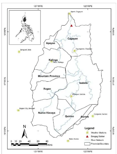
The Cagayan River Basin (CRB) is the largest river basin in the Philippines. It is located in the northeastern portion of the island of Luzon and between 15052’N-18023’N latitudes and 120051’E-122019’E longitudes (Figure 1). CRB has a drainage area of approximately 27,700 km2 covering the provinces of Regions 2, Cordillera Autonomous Region (CAR) and small parts of Region 3 (RBCO, 2007).
2.2. Climate, Topography and Physiography
CRB falls under Type III climate zone which is characterized by no pronounced maximum rain period and a short dry period (BRS-DPWH, 2002). According to PAGASA (2009), the northern part of the basin has an average annual rainfall of 1,000 mm and 3,000 mm in the southern mountains. The mean annual temperature and average relative humidity are 23.6-26.00C and 75-85%, respectively (DPWH & JICA, 2001).
Figure 1. The Cagayan River Basin, its provinces, the Bangag Station, and weather stations.
2.4. Land use/Land cover: About 37% of the area is covered by forest while grassland, agricultural area, and other land use such as settlement and water area occupies 34%, 27% and 2%, respectively. Of the 741,000 hectares of agricultural area, 94% are crop fields while the rest are fruit trees. The crop fields are further subdivided into 68% paddy field, 22% corn field and 10% upland crop field (DPWH & JICA 2001).
3. MODEL DESCRIPTION
The Soil and Water Assessment Tool (SWAT) model is a river basin scale model specifically used in predicting the effect of land management practices, over long periods of time, on variables such as flow and sediment to areas of varying soils, land use and management conditions. It is physically based, uses readily available inputs, computationally efficient and enables users to study long-term impacts (Neitsch et. al, 2005). The study used the SWAT 2005 version via the ArcSWAT interface for ArcGIS™.
SWAT is a continuous time model and is not designated to simulate detailed single-event flood routing (Neitsch et. al, 2005) and operates on a daily time step (Hao et. al, 2003). To predict surface runoff yield, the model uses a modified version of the SCS CN method (USDA-SCS, 1972):
Q
R 2S
R 0.8S
R 0.2S2
(1)
Q
0
R
0
.
2
S
(2)where Q and R are the daily surface runoff and daily rainfall, respectively, both in mm H2O. S is a retention parameter which varies spatially under various soil, land use, management and slope conditions, and temporally to respond to changes in soil water content (Hao et. al, 2003). The retention parameter is related to the curve number (CN) and defined as:
25.4 1000 10 CN S
(3)
The model estimates erosion and sediment yield from each sub-basin using the Modified Universal Soil Loss Equation (MUSLE) (Williams, 1995):
sed
Qsurfqpea kareahru
KCPLSCFRG 56. 0
8 .
11
(4)
where sed is the sediment yield on a given day in metric tons, Qsurf is the surface runoff volume in mmH20/ha, qpeak is the
peak runoff rate in m3/s, areahru is the area of the HRU in ha, K
is the USLE soil erodibility factor, C is the USLE cover and management factor, P is the USLE support practice factor, LS is the USLE topographic factor and CFRG is the course fragment factor. For a detailed description of these variables, the reader may refer to the theoretical documentation of SWAT 2005 (Neitsch et. al, 2005).
4. METHODOLOGY
The general procedure used in the study can be seen in Figure 1. Several datasets are inputted to the model after data preparation. The basin is automatically delineated via the SWAT model interface (ArcSWAT) using the input DEM while subbasins and finer subdivisions in the basin called the hydrologic response units (HRU) are defined by setting threshold limits for land use/land cover, soil type and slope class. Available flow and sediment data were used to calibrate and validate the model. The calibrated model was then rerun for five scenarios, the results of which are compared and became the basis of the author’s final analysis.
4.1. Data Preparation, Input and Model Setup
4.1.1. Digital Elevation Model: The Shuttle Radar Topography Mission Digital Elevation Model (SRTM-DEM) was used for the DEM requirement of SWAT. SRTM data are products of processed raw radar signals spaced at different intervals at the Jet Propulsion Laboratory (JPL) (USGS, 2011). The DEM used was a 3 arc-second medium resolution elevation data (approx. 90 m) resampled using cubic convolution interpolation and downloaded at the EarthExplorer website (URL: http://edcsns17.cr.usgs.gov/NewEarthExplorer). The DEM was used to generate percent slope values, to do automatic watershed delineation and in defining stream networks and gage outlets.
4.1.2. Land Cover/Land Use Map was generated from two sets of Landsat 7 TM and ETM+. CRB covers three Landsat scenes within the coverage of path 116, rows 47, 48 and 49. These satellite imageries passed through a processing scheme as shown in Figure 2. All downloaded Landsat ETM+ images were Level 1T products in Geographic Tagged Image-File Format (GeoTIFF). These were geo-referenced to include terrain correction that corrected parallax error from local topographic relief with a digital elevation model (Helmer & Ruefenacht, 2007).
Figure 2. The general procedure adopted in the study.
classify the reference images. Maximum likelihood was the final classifier used for image classification since it produced the highest over-all accuracy and a kappa coefficient () nearest to a value of 1 (Table 1). The overall accuracy should be at least 85% as prescribed by Anderson et. al (1976) while the value for is preferably close to 1.00 for this represents a situation where the classification is perfectly superior to random assignment of classes (Gao, 2009). The resulting classified image was post-processed using Majority Analysis in ENVI™ to eliminate “salt and pepper” effects.
The of LULC map using the more recent image set for the Cagayan River Basin is shown in Figure 3. Additionally, Table 2 shows the user-defined LULC classes and their corresponding SWAT LULC classes.
Table 1. Different classifiers used in the study and their overall accuracy and kappa coefficient values.
CLASSIFIER OVER-ALL
ACCURACY
KAPPA COEFFICIENT
Maximum Likelihood 91.07 0.88
Parallelepiped 47.66 0.34
Minimum Distance 85.77 0.87
Mahalanobis Distance 88.62 0.87
ISODATA 64.75 0.73
K-Means 64.75 0.73
Table 2. User-defined and SWAT LULC classes. USER-DEFINED
LULC
SWAT
LULC CODE DESCRIPTION
Unclassified AGRL Agricultural Land Generic
Built-up URML Residential-Medium to
Low Density
Bare soil RNGE Range-Grasses
Water WATR Water
Vegetation AGRR Agricultural-Row Crops
Forest FRST Forest-Mixed
4.1.3. Soil Dataset was generated from the Pit Profile Descriptions (PPD), Laboratory Analysis (LA) and Auger Boring Descriptions (ABD) of Cagayan, Isabela and Nueva Vizcaya Provinces from the Bureau of Soils and Water Management (BSWM).
4.1.4. Weather Stations. Three main weather stations located in Cagayan and Isabela provinces were used in the study. These stations have daily and monthly rainfall, humidity and temperature (minimum and maximum) data obtained from the Philippine Atmospheric, Geophysical and Astronomical Services Administration (PAGASA). Three additional rainfall stations located in Kalinga, Abra and Benguet from PAGASA and two additional precipitation data from stations in the Aurora province were also used from the Weather Underground (http://www.wunderground.com). The eight weather stations are shown in Figure 1. The weather data were obtained in text format and reformatted for SWAT input.
4.1.5. Climate Change Data.
The A1B and A2 climate
change scenarios are utilized in the study. Data for these two scenarios are extracted from PAGASA’s run of the Providing
Regional Climates for Impact Studies (PRECIS) model which generated projected changes in seasonal mean temperature (0C) and rainfall (%) (PAGASA, 2010). These projected incremental changes in rainfall and temperature are inputted to the model by editing the RFINC(mon) and TMPINC(mon), respectively, in the .SUB files of the SWAT model.
4.1.5. River Discharge and Sediment Data. Flow and sediment of the CRB are calibrated and validated at the Bureau of Research and Standards (BRS) station located in Bagag, Lal-lo, Cagayan (Figure 1). This station is selected because of its proximity to the main outlet of the basin. Streamflow and sediment data for this station are obtained from BRS-DPWH (2002).
4.2. Sensitivity Analysis. SWAT parameters will have to undergo sensitivity analysis first before model calibration to help in identifying and ranking parameters that have significant impact on specific model outputs such as streamflow and sediment yield (Saltelli et. al, 2000). The most sensitive parameters for flow are the Baseflow alpha factor (Alpha_BF), Initial SCS runoff curve number for moisture condition II (CN2) and the threshold depth of water in the shallow aquifer required for return flow to occur (Gwqmn). For sediments, the most sensitive parameters are the linear parameter for calculating the maximum amount of sediment that can be reentrained during channel sediment routing (Spcon), Exponent parameter for calculating sediment reentrained in channel sediment routing (Spexp) and the USLE equation support practice factor (Usle_P). These parameters are given priority in manual adjustments since minor adjustments in their values can translate to significant change in simulated values.
4.2. Model Performance Evaluation
The model was evaluated using four quantitative statistics as recommended and used by Moriasi et. al (2007) and Duan et. al (2009). These statistics are the Nash-Sutcliffe efficiency (NSE), percent bias (PBIAS), ratio of the root mean square error to the standard deviation of measured data (RSR) and the coefficient of determination (R2). (Moriasi et. al, 2007). Tables 4-5 provides a summary of model performance during model calibration and validation in different time steps.
4.3. Model Calibration and Validation.
Table 3. Default and Final Values of SWAT calibration parameters for flow and sediment.
Variable Parameter File iMet* Range Default Value Final Value
Flow Alpha_Bf .gw 1 [0, 1] 0.048 0.26
Ch_K2 .rte 1 0-150 0 25
Cn2 .mgt 3 [-25, 25] varied by LU 1.23745
Esco .hru 1 [0, 1] 0 1
Gwqmn .gw 2 [0,1000] 0 -263.22
Sediment Ch_Cov .rte 1 [0, 1] 0 0.601
Ch_Erod .rte 1 [0, 1] 0 0.400
Spcon .bsn 1 [0.0001, 0.01] 0.0001 0.003
Spexp .bsn 1 [1, 2] 1 1.420
Usle_P .mgt 1 [0, 1] 1 0.981
Usle_C crop.dat 3 [-25, 25]
0.25 0.233**
0.3 0.279***
0.01 0.009****
* variation method: 1 = replacement of initial parameter by value, 2 = adding value to the initial parameter, 3 = multiplying initial parameter by a value in percentage
** for AGRL ; *** for AGRR; **** for FRST
of data. For model calibration, the 1984 daily stream flow (in liters/sec) data and 2002-2005 monthly sediment (in ppm) data are used. Meanwhile, the 1985-1986 daily stream flow data and 2006-2007 monthly sediment data are used for model validation. Daily stream flow data for years 1984 and 1985 are used because these are the only period with almost complete records. BRS do not have daily records for sediments. Only monthly records are available for sediment data and the period with the most number of records are 2002-2007. No sediment data are available for years earlier than 2002 and data for years later than 2007 are fragmental (i.e., more than six months are without data). The final values of sediment parameters and five most sensitive flow parameters are shown in Table 3. Plots of the observed and simulated flow and sediment yields are shown in Figures 4 and 5.
Table 4. Model Performance during calibration.
Variable Calibration
Period Time Step NSE R2 RSR PBIAS
Flow 1984 Daily 0.89 0.74 0.34 17.64
Monthly 0.47 0.83 0.73 17.75
Sediment 2002-
2005
Monthly 0.96 0.93 0.20 -7.30
Annual 0.99 0.97 0.11 -12.31
Table 5. Model Performance during validation.
Variable Validation
Period Time Step NSE R2 RSR PBIAS
Flow 1984 Daily 0.89 0.74 0.34 17.64
Monthly 0.47 0.83 0.73 17.75
Sediment 2002-
2005
Monthly 0.96 0.93 0.20 -7.30
Annual 0.99 0.97 0.11 -12.31
5. RESULTS AND DISSCUSSION
5.1. Base Scenario
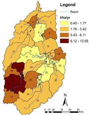
The soil loss rate map derived from sediment yield for the base scenario is shown in Figure 3. The minimum and maximum values for this scenario are 0.45 ton ha-1 yr-1 and 12.05 ton ha-1 yr-1 which correspond to subbasins 28 and 21, respectively. The simulated maximum value is beyond the upper limit of tolerable soil loss of 11.2 t ha-1 yr-1 according to Hudson (1995) as cited by Alibuyog et. al (2009). Subbasin 28 is characterized by a relatively flat terrain with the whole area having slope less than or equal to 17% and predominantly an agricultural area (AGRR) while most of the subbasin 21 area have steep slopes (>17%) and with almost equal distribution of RNGE, AGRR and FRST areas.
Figure 3. Soil loss rate map of the basin under the base scenario.
5.2. Model Simulation incorporating Climate Change
Climate change data are incorporated in the model by inputting the projected seasonal change in rainfall and temperature for each subbasin. After manipulating the subbasin parameters for climate change analysis (RFINC and TMPINC), the calibrated model was rerun for two scenarios (A1B and A2) each under two time slices centered at year 2020 and 2050. These two scenarios have been the focus of climate change model inter- comparison studies according to IPCC (2007). The average total generated sediment yield of the whole basin for this run is shown in Figure 6a.
5.3. Model Simulation incorporating Land Use/Land Cover Change
The projected land cover change rates derived from subtracting the sets of Landsat images are inputted to the model by modifying the individual HRU files (with file extension *.hru) for each subbasin. The calibrated model is rerun with the modified HRU files and the average sediment yield for the simulation period is evaluated. The result of this run is also shown in Figure 6a.
5.4. Model Simulation incorporating Climate Change and Land Use/ Land Cover Change
Figure 4. Observed and simulated discharge (flow) and sediment at Bangag station during model calibration.
Figure 5. Observed and simulated discharge (flow) and sediment at Bangag station during model validation.
the calibrated model was executed to simulate the combined effects of climate change and land use/land cover change to the sediment yield of the Cagayan River Basin. The results of this run are also shown in Figures 6a and 6b.
5.5. Model Simulation incorporating land cover-based mitigation measures
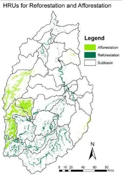
The study used riparian reforestation and afforestation of hilly and mountainous areas as two land cover-based mitigation measures. Important SWAT input files (e.g., *.mgt, *.sol, *.hru) were modified to reflect these land cover changes. These mitigation measures were applied to the model under the four previously mentioned scenarios in Sections 5.1 to 5.4. Figure 7 shows the spatial distribution of HRUs where these mitigation measures are applied while Figure 6b shows their effect on the generated sediment yield of the basin.
6. ANALYSIS AND DISCUSSION OF RESULTS
6.1. The Effects of LULC and Climate Changes on the Sediment Yield of the Cagayan River Basin
The Cagayan River Basin was found to have a total average annual sediment yield of 114.76 ton ha-1 yr-1 under the base scenario that is, if the present land use/land cover (LULC) distribution of the basin were to use in model simulation. This simulated sediment yield agrees with the reported observed range of average erosion rate for Regions CAR, I and II possibly due to the projected lesser rainfall and less increase in temperature compared to its counterpart for the year 2050 (A2 2050) and scenario A1B. It should be noted, however, that the same scenario will eventually produce an increase in sediment yield if coupled with LULC change (A220LC in Figure 6a).
In general, it has been demonstrated that sediment yield will increase if the current LULC change rate and projected change in the climatic parameters in the Cagayan River basin would persist and climate change scenario A1B would bring a higher increase in sediment yield compared to the A2 scenario.
6.2. Effects of Applying Proposed Mitigation Measures
The land cover-based mitigation measures applied to both climate change scenarios with LULC change have produced lesser sediment yields compared to the base scenario (Figure 6b) by about -26.3% to -45.32%. It is interesting to note that the highest generated sediment yield (157.21 t ha-1 yr-1 under A1B50LC scenario) was decreased to 109. 44 t ha-1 yr-1 which was lower than the current sediment yield of the basin (114.76 t ha-1 yr-1) under the base scenario. This demonstrated how riparian reforestation and afforestation of hilly and mountainous areas have successfully mitigated the ill-effects of climate change to the sediment yield of the Cagayan river basin even if coupled with LULC change.
7. CONCLUSIONS
The study has demonstrated how the integration of SWAT model, Remote Sensing and GIS can be a powerful tool in simulating watershed variables such as the sediment yield of a large river basin. Moreover, the study has validated the applicability of the model in simulating flow and sediment discharge dynamics of the Cagayan river basin based on the satisfactory values of the statistical measures of model efficiency. Lastly, climate change data were successfully utilized to quantify the impact of changes in the climate regime to the sediment yield of the study basin.
REFERENCES
(a) (b)
Figure 6. Simulated sediment yield of the basin under different scenarios: (a) BS=Base Scenario, LC=land use/land cover change scenario, codes for other scenarios: A1B=climate change scenario A1B, A2= climate change scenario A2, 20=corresponds to year 2020, 50=corresponds to year 2050 (e.g., A1B20LC= climate change scenario A1B at year 2020 with land use/land cover change scenario); (b) Comparison of sediment yields generated
before and after applying mitigation measures.
Figure 7. The HRUs where mitigation measures (afforestation and reforestation) were applied.
Alibuyog, N. R., Ella, V. B., Reyes, M. R., Srinivasan, R., Heatwole, C., & Dillaha, T., 2009. Predicting the Effects of land Use on Runoff and Sediment Yields in Selected Sub-watersheds of the Manupali River
Using the ArcSWAT Model. Soil and Water Assessment Tool (SWAT):
Global Applications, pp. 253-266.
BRS-DPWH, 2002. Water Resources Region No. 2 CAGAYAN VALLEY, BRS-DPWH, Quezon City, PHL.
CAD-PAGASA, 2004. DOST Service Institutes “Climate Change
Scenario for the Philippines”.
http://kidlat.pagasa.dost.gov.ph/cab/scenario.htm. (27 October 2011).
DPWH & JICA, 2001. The Feasibility Study of the Flood Control Project for the Lower Cagayan River in the Republic of the Philippines
“Present River Condition”.
http://www.dpwh.gov.ph/infrastructure/JICA2/. (14 May 2010)
Duan, Z., Xianfeng, S., & Liu, J. (2009). Application of SWAT for sediment yield estimation in a mountainous agricultural basin. In:
International Conference on Geoinformatics, pp. 1-5.
Gao, J., 2009. Digital Analysis of Remotely Sensed Imagery. McGraw-Hill, USA.
Gupta, H. V., Sorooshian, S., & Yapo, P. O., 1999. Status of automatic calibration for hydrologic models: Comparison with multilevel expert calibration. J. Hydrologic Eng. 4(2), pp. 135-143.
Hao, F., Zhang, X., Cheng, H., Liu, C., & Yang, Z., 2003. Runoff and Sediment Yield Simulation in a Large Basin using GIS and a
Distributed Hydrological Model. GIS and Remote Sensing in
Hydrology, Water Resources and Environment, China, pp. 157-166.
Hudson, N., 1995. Soil Conservation. BT Batsford Limited, London.
IPCC. 2007. Climate Change 2007: Synthesis Report. Cambridge University Press, New York.
Jabines, A., & Inventor, J., 2007. The Philippines: A Climate Hotspot Climate Change Impacts and the Philippines. Greenpeace Southeast Asia, Quezon City, PHL.
Martinuzzi, S., Gould, W. A., González, R., & M., O., 2006. Creating cloud-free Landsat ETM+ data sets in tropical landscapes: cloud and cloud-shadow removal. USDA, FS, IITF.
Moriasi, D. N., Arnold, J. G., Van Liew, M. W., Bingner, R. L., Harmel, R. D., & Veith, T. L., 2007. Model Evaluation Guidelines for Systematic Quantification of Accuracy in Watershed Simulations.
Transactions of the ASABE, 50(3), pp. 885-900.
Neitsch, S. L., Arnold, J. G., Kiniry, J. R., & Williams, J. R., 2005. Soil and Water Assessment Tool Theoretical Documentation Version 2005. Agricultural Research Service and Texas Agricultural Experiment Station, Temple, Texas.
PAGASA, 2009. Hydrometeorology “Basin Information - Cagayan River Basin”. http://www.weather.gov.ph (May 2010)
PAGASA, 2010. MDG-F 1656 Fact Sheet #1. Communicating Climate Information for Effective Development Planning. MDG Achievement Fund, Quezon City.
RBCO, 2007. Water Environment Partnership in Asia (WEPA) “Plans and Programs of River Basin Control Office Relative to Water Resources Management and River Basin Management.” www.wepa-db.net/pdf/0710philippines/8_RBCO.pdf (14 May 2010)
Saltelli, A., Scott, E., Chan, K., & S., M., 2000. Sensitivity Analysis. John Wiley & Sons, Chichester.
Solidum, R. U., 2011. Vulnerability and Resiliency of Megacities to Climate Change and Natural Disasters. In: International Conference on
Green Urbanism 2011: Planning Greener Cities. Manila, PHL.
USDA-SCS, 1972. Hydrology Section 4. In “National Engineering
Handbook”. USDA, Soil Conservation Service, Washington, DC, USA.
USGS, 2011. Earth Resources and Observation Science (EROS) Center “Shuttle Radar Topography Mission (SRTM)-Finished”.http://eros.usgs.gov/#/Find_Data/Products_and_Data_Availa ble/SRTM (09 Sept. 2011).
Williams, J. R.,1995. Computer Models of Watershed Hydrology
Chapter 25: The EPIC Model. (V. P. Singh, Ed.), pp. 909-1000.
ACKNOWLEDGEMENTS