The Impact of School Structure on Student
Outcomes
Kelly Bedard
Chau Do
A B S T R A C T
While nearly half of all school districts have adopted middle schools, there is little quantitative evidence of the efficacy of this educational structure. We estimate the impact of moving from a junior high school system, where stu-dents stay in elementary school longer, to a middle school system for on-time high school completion. This is a particularly good outcome measure because middle school advocates argued that this new system would be especially helpful for lower achieving students. In contrast to the stated objective, we find that moving to a middle school system decreases on-time high school completion by approximately 1–3 percent.
I. Introduction
Beginning in the 1940s, educational reformers began pushing for the creation of junior high schools. They argued that specialized schools for students in Grades 7–9 would better prepare young adolescents for high school by exposing them to a high school-like environment without the trauma of placing them in the same building as older teenagers. By the late 1960s, middle school supporters were simi-larly arguing that sixth grade students would benefit from being separated from ele-mentary school children. They believed that the social, psychological, and academic needs of young adolescents are distinct from young children and older youth (National Middle School Association 1995). Thus, placing young adolescents with high school students hinders social development, while placing them with elementary school students slows academic progress. They therefore argued that middle school
Kelly Bedard is an assistant professor of economics at the University of California, Santa Barbara and Chau Do is an economist with the Office of the Comptroller of the Currency, Risk Analysis Division, Financial Access and Compliance. The authors thank Olivier Deschênes, Peter Kuhn, Cathy Weinberger, and two anonymous referees for their comments and suggestions. The data used in this article can be obtained beginning January 1, 2006 through December 31, 2008 from Kelly Bedard, Department of Economics, University of California, Santa Barbara CA 93106-9210, Kelly@econ.ucsb.edu. [Submitted September 2003; accepted September 2004]
ISSN 022-166X E-ISSN 1548-8004 © 2005 by the Board of Regents of the University of Wisconsin System
systems have lower dropout rates relative to junior high school systems (National Center for Education Statistics (NCES) 2000; Clark and Clark 1993). This new round of educational reform advocated middle schools spanning Grades 5 or 6 through 8 and high schools serving Grades 9–12 (NCES 2000; Goldin 1999).
A simple accounting of school configurations over time suggests that middle school advocates have won the battle (see Table 1). In 1986, 33 percent of sixth graders were enrolled in middle schools serving Grades 5 or 6 through 8; by 2001 this number had grown to 58 percent. Given the explicit nature of the claims made by middle school advocates, and the massive shift from junior high schools to middle schools over the past 15 years, it is somewhat surprising that economists have completely ignored this potentially important structural change.
This study provides the first estimate of the net impact of the movement to middle schools for on-time high school completion (this measure is defined in Section IIIB), which is an important measure of educational success for the bottom of the ability dis-tribution. More specifically, we use data on school configurations and on-time high school graduation rates from the NCES Common Core of Data (CCD) covering all U.S. schools and fixed effects estimation to isolate the impact of middle school adop-tion from other factors influencing high school compleadop-tion rates. We find that the movement to a middle school system is associated with a 1–3 percent fall in the on-time high school completion rate. This is a surprising result for a program with the stated aim of aiding less able students. Moreover, since high school dropouts earn lower wages (Cameron and Heckman 1993), are more likely to be unemployed (Rees 1986), and more likely to participate in criminal activities (Freeman 1996), the nega-tive economic implications of less on-time high school completion may be far reach-ing and multifaceted.
The remainder of the paper is as follows. The next section outlines the avenues through which middle schools might impact student outcomes. Section III describes the data and the school district panel. Section IV documents the movement to middle schools. Section V presents the estimation strategy and results. Section VI concludes.
II. Potential Impact of Middle Schools
For expository ease, in this section we assume that elementary/junior high/high school systems are configured as Grades K–6/7–8/9–12, and that elemen-tary/middle/high school systems are configured as Grades K–5/6–8/9–12 (we allow for other configurations in the empirical analysis, see Sections IIIA and VD). Within this simple framework, restructuring a school district from an elementary/junior high/high school system to an elementary/middle/high school system simply entails moving sixth graders out of elementary school a year earlier. While this may seem like a small change, it implies several important structural changes that may impact long-run student outcomes.
It is easiest to think about this issue within a simple education production frame-work. Student outcomes, Y,are a function of peer effects, teacher effectiveness, cur-riculum, school attributes, and student characteristics, including ability.
(1) Y= f(peers, teachers, curriculum, schools; individual characteristics)
The Journal of Human Resources
Table 1
School Configurations
Percent of Fifth Graders Percent of Sixth Graders Percent of Ninth Graders
School Type 1986 1994 2001 1986 1994 2001 1986 1994 2001
All Students
K–5 27.9 42.5 48.2 — — — — — —
K–6 43.8 30.9 24.6 43.6 30.4 22.1 — — —
K–8 6.4 5.2 5.7 6.6 5.5 6.0 — — —
3–5 1.7 3.0 3.3 — — — — — —
4–6 2.8 2.5 2.2 2.7 2.5 2.1 — — —
5–6 2.2 2.3 3.2 2.2 2.4 3.3 — — —
5–8 4.0 4.3 4.2 4.2 4.8 5.0 — — —
6–8 — — — 28.8 44.7 52.6 — — —
7–9 — — — — — — 16.9 7.8 4.3
7–12 — — — — — — 7.1 6.3 4.9
8–9 — — — — — — 2.0 1.1 1.0
8–12 — — — — — — 2.2 1.7 2.8
9–12 — — — — — — 66.4 76.4 80.5
Other 11.3 9.5 8.7 11.7 9.8 8.9 5.4 6.7 6.5
Bedard and Do
663
Students in Unified Districts
K–5 29.0 44.1 50.4 — — — — — —
K–6 43.8 30.1 23.5 43.5 29.6 21.2 — — —
K–8 5.4 4.2 4.6 5.6 4.5 4.8 — — —
3–5 1.7 2.9 3.3 — — — — — —
4–6 2.8 2.5 2.1 2.8 2.5 2.1 — — —
5–6 2.2 2.3 3.3 2.3 2.4 3.3 — — —
5–8 3.9 4.3 4.2 4.1 4.7 5.0 — — —
6–8 — — — 29.7 46.1 54.4 — — —
7–9 — — — — — — 17.9 8.3 4.5
7–12 — — — — — — 7.4 6.6 5.0
8–9 — — — — — — 2.1 1.2 1.1
8–12 — — — — — — 2.3 1.8 2.9
9–12 — — — — — — 64.8 75.3 79.8
Other 11.2 9.6 8.6 11.9 10.1 9.1 5.4 6.8 6.7
Equation 1 highlights the reason that it is difficult, a priori, to predict the impact of middle schools on student outcomes—school structure impacts school attributes directly as well as affecting peer groups, curriculum, and teacher characteristics indi-rectly through student body composition changes and possibly through interactions between variables depending on the functional form of the production function (which is unknown).
At the most basic level, middle schools move eleven-year-olds out of relatively small elementary schools where they are the oldest students in the school, and spend most of their day with the same group of students and one teacher, to a substantially larger institution where they are the youngest students in the school and have many different teachers during the course of each school day. This change in structure has several potentially important implications. First, sixth graders are now more likely to be instructed by “experts” with more training in specific subjects—which likely has a positive impact. Second, monitoring is more difficult given the larger student body and the fact that each teacher instructs several different groups of students each day— which likely has a negative impact.
Third, and more ambiguously in terms of impact, the fact that middle schools have many classes at each grade level allows them to do more ability-tracking than in elementary schools (see Mills 1998 and the references therein). As tracking may benefit some students at the expense of other students, it is unclear whether middle schools are facilitating better outcomes in this regard. In particular, whether track-ing benefits high-ability students at the expense of low-ability students is the sub-ject of some debate (Hoffer 1992; Argys, Rees, and Brewer 1996; Figlio and Page 2002).
Fourth, and also ambiguously in terms of impact, is the switch from being the oldest to the youngest in the school. On the one hand, exposure to older students may benefit sixth graders if they are exposed to more mature behavior. On the other hand, immature sixth graders may find being the youngest students in the school traumatic.
Finally, middle school adoption may change retention patterns. It is possible that sixth graders are more likely to be retained in middle schools than in elementary school because teachers and administrators are reluctant to hold the “oldest” children, preferring to pass them onto the next school where they can be retained the next year when they are relatively “young.” Assuming that these children would have been retained in Grade 7 in the absence of a middle school, middle schools then simply change the timing of retention. Whether this change in timing has a positive, negative, or zero impact is unclear (we return to this issue in Section IIIB).
Given the possible positive and negative aspects of middle schools, the net effect is an empirical question. Using CCD, we estimate the net effect of middle schools on a particular student outcome—on-time high school completion. This is a particularly interesting measure because middle school advocates claimed that middle schools would be especially beneficial for weaker students, and high school graduation is only a reasonable a measure of success for weaker students.
III. Data
All data are from the NCES CCD. We obtain district level high school completion counts from the Public Education Agency Universe from 1992/1993–2000/2001 and school configuration (grades served) and grade-by-grade enrollment data from the Public School Universe Data from 1987/1988–1993/1994. Combining these sources allows us to construct an eight-year district level panel by matching district specific middle school placement rates to the appropriate on-time high completion rate approximately seven years later. The on-time high school com-pletion rate is defined as the number of diplomas conferred to each sixth grade class six years and ten months later (for expository ease, throughout the paper this will be denoted as seven years) at the scheduled “on-time” end of Grade 12 divided by the population of fifth grade students eight years earlier (see Section IIIB for a detailed explanation for the choice of denominators). The middle school placement rate is the percentage of sixth graders in middle schools (see Section IIIA). For expository ease all cohorts are identified by the beginning of their sixth grade year. For example, the cohort that entered Grade 6 in the fall of 1987 and potentially finished high school in the spring of 1994 is referred to as the 1987 cohort (t= 1987).
We restrict the sample to unified districts that serve kindergarten through Grade 12 to facilitate the matching of sixth graders with high schools. This restriction excludes approximately 250 high school districts and 4,000 elementary districts (see Table 2). While these may seem like large exclusions, on average 91 percent of students are in unified districts in each year. Communities with separate elementary and high school districts are problematic because an elementary district might send students to multi-ple high school districts, and high school districts may similarly receive students from several elementary districts. This multi-directionality precludes us from identifying the entire educational path of the students involved and forces us to focus on unified districts. However, to the extent that students from public elementary districts and pri-vate elementary schools are flowing into unified districts to attend high school, we may still be mismeasuring middle school rates. That said, these flows will only bias our fixed effects estimates if they change at middle school adoption dates.
Unfortunately, some districts report sporadically, making it difficult to identify the timing of middle school adoptions and exacerbating measurement error (we return to this issue in Section V). As such, the base specification further restricts the sample to districts that report in all years. This eliminates 2,055 districts, but only 13 percent of students—78 percent of students are in unified districts that report the required infor-mation in all years. Further, as we discuss below, the excluded districts appear to be observationally equivalent to the included sample of unified districts, and all results are similar when these districts are included (see Section VA).
A. Middle Schools
Ascertaining the impact of middle schools requires a working definition of a middle school. Because school districts use a variety of configurations, deciding upon such a definition is not as simple as it might seem. However, middle schools are most often defined by the exclusion of ninth graders and the inclusion of fifth or sixth graders.1 We therefore define middle schools as institutions spanning Grades 5 through 8 or 6 through 8, with the vast majority of middle schools being the later (see Table 1).
District-level high school completion data provide no way of identifying high school students coming from middle schools separately from those coming from other types of schools. We therefore measure the pervasiveness of middle schools within a district as the proportion of a district’s sixth graders attending middle schools.
( ) M
where Sdenotes the number of students, Mis the fraction of sixth graders in middle schools, idenotes district and tdenotes year. As such, Sitmiddle6this the total number of sixth graders in middle schools in a district in a given year and Sittotal6this the total number of sixth graders in a district in a given year.2This measure also allows for the
fact that while some districts switch from no middle schools to placing all students in middle schools at a single point in time, other districts switch gradually over time and/or partially shift. For example, a district might switch half their sixth grade stu-dents to middle schools in one year and the other half five years later, or they may never switch the other half. Of course, some districts also shift away from middle schools.
For comparative purposes, Table 2 reports the proportion of sixth graders in the balanced unified sample, all unified districts, and all districts that include sixth graders. Two points warrant comment. First, in all samples, the percentage of sixth graders in middle schools rises approximately 16 percentage points from 1987 to 1994. This is a substantial increase in only eight years. Secondly, while the two uni-fied district samples are nearly identical, elementary districts are less likely to use middle schools. Only 12 percent of elementary districts used middle schools in 1987, and only 15 percent in 1994.
B. On-Time High School Graduation
The graduation rate is defined as the proportion of fifth grade students receiving a reg-ular diploma at the end of their senior year.
( ) G
where Gis the on-time graduation rate, Cis the number of students conferred diplo-mas in year t+7, and Sit−1total5this the number of fifth graders in the district in year
Bedard and Do
667
Table 2
Middle School Adoptions and High School Graduation Rates
Unified School Districts Districts with Districts with
(Complete Reporting) All Unified School Districts Twelfth Graders Sixth Graders
Grade 6 Grade % % % % % %
Entry 12 Exit Middle On-Time Middle On-Time On-Time Middle
Year Year Districts School Graduation Districts School Graduation Districts Graduation Districts School
1987 1994 8,456 0.36 0.79 9,448 0.36 0.80 9,714 0.79 13,611 0.35
(0.43) (0.23) (0.43) (0.24) (0.26) (0.43)
1988 1995 8,456 0.39 0.78 10,086 0.38 0.78 10,264 0.79 14,138 0.37
(0.44) (0.22) (0.44) (0.25) (0.25) (0.44)
1989 1996 8,456 0.41 0.77 9,885 0.41 0.77 10,060 0.77 14,066 0.40
(0.44) (0.21) (0.44) (0.22) (0.23) (0.44)
1990 1997 8,456 0.43 0.76 9,636 0.43 0.76 9,780 0.76 14,016 0.42
(0.45) (0.21) (0.45) (0.24) (0.27) (0.45)
1991 1998 8,456 0.46 0.76 10,143 0.45 0.76 10,312 0.76 13,902 0.44
(0.45) (0.21) (0.45) (0.23) (0.24) (0.45)
1992 1999 8,456 0.48 0.75 10,134 0.47 0.76 10,397 0.76 13,772 0.46
(0.44) (0.20) (0.45) (0.23) (0.49) (0.45)
1993 2000 8,456 0.50 0.76 10,104 0.50 0.76 10,392 0.76 13,671 0.48
(0.44) (0.20) (0.45) (0.24) (0.25) (0.45)
1994 2001 8,456 0.53 0.75 10,233 0.52 0.76 10,454 0.76 13,602 0.50
(0.44) (0.20) (0.45) (0.23) (0.36) (0.45)
t−1. Students who complete high school a year late or eventually obtain a GED are considered noncompletors. This is a reasonable measure of school district failure as it measures both noncompletion and slower than usual completion, both of which may be affected by middle school adoption.
As discussed in Section II, it is possible that middle school adoption increases sixth grade retention. Since only 4–5 percent of sixth graders are in middle schools span-ning Grades 5 through 8, and this fraction is essentially constant over the sample period, we use fifth grade enrollment in year t−1 as the base rather than sixth grade enrollment in year t,to avoid confounding retention and high school noncompletion. As a sensitivity check, we also use fourth grade enrollment in year t−2 and ninth grade enrollment in year t+3 as the denominator (see Section V).
In addition to ensuring that the on-time completion measure is not exaggerated by a switch from seventh grade retention to sixth grade retention due to middle school adoption, by selecting the appropriate denominator, one might also want to estimate the magnitude, and existence, of any increase in sixth grade retention resulting from middle school adoption. Unfortunately, this is not possible using the CCD because any impact on retention is not separately identifiable from possible changes in the entry point of students from private schools and elementary districts into unified dis-tricts. More concretely, students tend to flow into unified districts at the beginning of middle school, junior high school, and high school. As such, a switch from a junior high school to a middle school system means that some students enter in Grade 6 instead of waiting until Grade 7. On the other hand, some students may now wait and enter in Grade 9. As the CCD only reports total enrollment by grade, we cannot dis-entangle retention from the somewhat complicated changes in the timing of flows. However, two things are clear. One, middle school adoption does not affect fifth grade enrollment. And, two, the change in entry timing all happens within the sixth through ninth grade time frame. Together, these determine the choice of denominators.
We use on-time graduation rather than the dropout rate for two reasons. First, the dropout data in the CCD does not begin until 1992, and even then is only available for a limited number of states. Secondly, the CCD dropout measure includes students who leave during the regular school year but excludes those who simply do not reen-roll after a summer recess.
However, on-time completion, as defined in Equation 3, does have two drawbacks. First, we cannot distinguish students who leave school from those who move to another district. Secondly, some unified districts have substantial inflow from sur-rounding elementary districts at the ninth grade level. This is one reason for using ninth grade enrollment as the denominator in some specifications. However, these estimates should be viewed with some caution since middle school adoption often implies the movement of ninth graders to high schools and hence may imply moving tenth grade retention to Grade 9 for the same reasons that seventh grade retention might be accelerated to the Grade 6 (as discussed above). That being said, assuming that ninth grade enrollment is not the denominator in Equation 3, neither of these fac-tors will bias our fixed effects estimates unless the cross-district movement of high school students is coincidental with the movement toward or away from middle schools in unified districts, which is unlikely.
Bedard and Do 669
published NCES statistics,3the on-time high school graduation rate fell by approxi-mately 4 percentage points during the late 1980s and then leveled off for all subsam-ples. Remember, however, that it is only the trend in on-time completion that is consistent with the trend in the NCES dropout rate, and not the levels, since our mea-sure uses fifth grade enrollment in t−1 as the base, and hence includes the inflow of students between Grades 6 and 9, as excluding nontime completors who are included in the dropout rates reported by the NCES. Given this trend in on-time high school graduation, all models reported in the remainder of the paper include unrestricted state-specific year controls.
C. District Characteristics
In an attempt to control for the time-varying changes within districts that may affect high school graduation rates, all models also include the available measurable district characteristics: The number of administrators, teachers, librarians, guidance coun-selors, schools within a district, and teachers’ aids (with the exception of the number of schools, all are reported in per-pupil terms).4Table 3 reports summary statistics for all of the variables used in the analysis. The average district has 0.003 administrators and 0.059 teachers per student. Further, as all models also include unrestricted state-specific year indicators, statewide policy changes are also controlled for.
IV. The Movement to Middle Schools
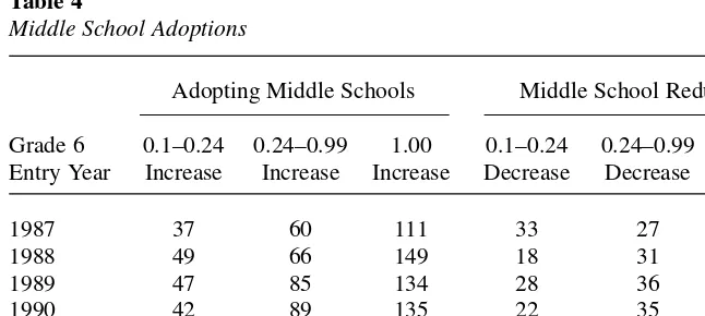
Before turning to the formal analysis, it is instructive to examine the pattern of middle school adoptions and abolitions over time. Toward this end, Table 4 reports the number of districts in which the fraction of sixth graders in middle schools increases or decreases by 10–24 percentage points, 25–99 percentage points and 100 percentage points. For descriptive purposes, in this section, we restrict attention to districts with 10 percentage points or greater changes to mitigate confounding middle school changes with measurement error (noise). Since middle school attendance is the ratio of sixth graders in middle schools over the total number of sixth graders in each district, misreporting of the numerator or the denominator and/or small annual fluctu-ations in sixth grade populfluctu-ations may cause the middle school percentage to vary slightly from year to year. We examine the impact of measurement error in Section VC.
Table 4 highlights three facts. First, there is substantial district-time variation in the adoption of middle schools. Approximately 400 districts either adopt or abolish mid-dle schools in each year. Secondly, a little under half of the districts that adopt midmid-dle
3. See http://nces.ed.gov/pubs2002/2002030.pdf.
schools did so incrementally while the remainder either moved all sixth graders into middle schools or out of middle schools at a single point in time. Finally, there are approximately three times as many adoptions as abolitions.
V. Panel Estimates
A. The Basic Fixed Effects Model
The objective is to estimate the impact of middle school adoption on the on-time high school completion rate.
Table 3
Descriptive Statistics
Mean Standard Deviation
On-time graduation 0.764 0.210
Percent in middle schools 0.449 0.445
Number of schools in district 85.0 195.3
Per Pupil
Administrators 0.003 0.001
Teacher 0.059 0.021
Librarians 0.001 0.001
Guidance counselors 0.002 0.001
Teachers’ aides 0.107 0.007
Sample size 67,648
Weighted by Grade 5 size in t − 1. Base sample is the balanced panel.
Table 4
Middle School Adoptions
Adopting Middle Schools Middle School Reductions
Grade 6 0.1–0.24 0.24–0.99 1.00 0.1–0.24 0.24–0.99 1.00 Entry Year Increase Increase Increase Decrease Decrease Decrease
1987 37 60 111 33 27 81
1988 49 66 149 18 31 56
1989 47 85 134 28 36 44
1990 42 89 135 22 35 68
1991 33 71 166 20 37 67
1992 41 76 183 22 37 73
1993 30 81 150 27 39 71
(4) Git+7= αi+ φt+ βMit+ γXit+ εit
where idenotes districts, t= 1987, . . . , 1994 (the sixth grade year for each cohort),
αis a vector of district fixed effects, ø is a vector of state-specific year indicators, X is a vector of time-varying district characteristics, and eis the usual error term. As described above, an important feature of middle school adoption is that they occurred in different districts in different years. This is helpful because it reduces the possibil-ity that the results are driven by a shift to middle schools at a single point in time that happens to coincide with some other unobserved change. It is also worth reempha-sizing that there are both middle school adoptions and abolitions, which means that we are not estimating the impact of middle schools off of a one-directional change. Stated somewhat differently, the district and time variation in adoption and abolition dates gives us more confidence in our identification strategy as it is unlikely that dis-tricts changing middle school rates in different years experience some other system-atic shock that would bring the control group into question.
The estimates for Equation 4 are reported in Table 5. The first row reports the pri-mary coefficient of interest, β-the impact of middle school adoption, and the defini-tions in Rows 4–9 report the dependent variable definition, the model specification, and the sample. Unless otherwise specified, all models are weighted by the square root of the base population, usually Grade 5 enrollment in t−1,5and all standard errors
are clustered by district.
The results for the base specification, the balanced panel, are reported in Column 1. This specification defines on-time graduation as the fraction of the fifth grade class in t−1 that receives a diploma in t+7. The coefficient estimate for the middle school variable implies that a 100 percentage point move toward middle schools reduces the on-time graduation rate by 0.8 percentage points. This impact is both statistically sig-nificant (standard error = 0.004) and economically important as it implies a 3 percent rise in the noncompletion rate, or at least not completing on time.
Column 2 replicates Column 1, but excludes years in which middle school changes occur. This specification is important because there are possible transitory effects associated with school structure changes that may confound the results. For example, if middle school adoption increases the fraction of sixth graders who are retained, the first cohort exposed to middle schools will be smaller than subsequent cohorts due to a change in the flow from grade to grade, which will take one year to settle into the new pattern. The results presented in Column 2 show that the results in Column 1 are robust to such transitory effects. While the point estimate excluding the year of the change is somewhat larger, the difference is not statistically significant. As a final check for transitory effects, Column 3 also excludes the year after a change. Again, the results are similar.
Even though using the fifth grade class size in year t−1 avoids confounding the impact on sixth grade retention and on-time completion, we nonetheless use fourth grade class size in year t−2 and ninth grade class size in year t+3 as the base popu-lations in constructing on-time completion as sensitivity checks. We do not use Grade 6 in year tas the base as it may be contaminated by changes in Grade 6 retention.
Bedard and Do 671
The Journal of Human Resources
Table 5
The Impact of Middle School Adoption for On-Time High School Graduation
(1) (2) (3) (4) (5) (6) (7) (8) (9) (10)
Percent 6th graders −0.008 −0.011 −0.012 −0.007 −0.005 −0.013 −0.007 −0.022 −0.008 −0.010 in middle schools (0.004) (0.005) (0.007) (0.004) (0.002) (0.004) (0.004) (0.010) (0.039) (0.004)
One-year lead in 0.000 0.000
middle school (0.004) (0.004)
adoption
Two-year lead in 0.005
middle school (0.004)
adoption
Completion Diploma Diploma Diploma Diploma Diploma Grade 12 Diploma Diploma Diploma Diploma definition
Base population Grade 5 Grade 5 Grade 5 Grade 4 Grade 9 Grade 5 Grade 5 Grade 5 Grade 5 Grade 5
Balanced Yes Yes Yes Yes Yes Yes No Yes Yes Yes
Weighted Yes Yes Yes Yes Yes Yes Yes No Yes Yes
Excludes year No Yes Yes No No No No No No No
of change
Excludes year No No Yes No No No No No No No
After change
R-squared 0.69 0.69 0.69 0.76 0.74 0.66 0.65 0.50 0.69 0.71
Sample size 67,648 63,402 52,914 59,815 74,889 73,080 79,669 67,648 67,583 59,108
The results are reported in Columns 4 and 5. Again, the point estimates are statisti-cally significant and very similar to the base specification.
As with most administrative data, some variables are more regularly reported than others. In the case of NCES, twelfth grade enrollment is more regularly reported than the number of conferred diplomas. Since approximately 20 percent of a ninth grade class leaves school and/or repeats a grade before Grade 12, using on-time Grade 12 enrollment as a measure of completion is an attractive specification check in light of the more regular reporting. The results for this specification are reported in Column 6. Consistent with all previous results, the point estimate for this specification implies that a 100 percentage point move toward middle schools reduces on-time Grade 12 enrollment by 1.3 percentage points (standard error = 0.004).
Columns 7 and 8 check that the sampling restrictions and weights are not driving the results. In Column 7 we report the results for the unbalanced panel, including all available observations, adding data for 2,055 districts with incomplete reporting (increasing the sample size by 12,021 observations). The results are almost identical to the base specification. Column 8 then replicates Column 1, but unweighted with heteroskedastic consistent standard error. In the absence of weights, the point estimate for the middle school variable rises to 2.2 percent (standard error = 0.010).
B. Endogenous Middle School Adoption
The analysis of the impact of middle school adoption on student outcomes raises the question of endogeneity. More concretely, one may be concerned that our results partly reflect the decision of “in-trouble” districts to adopt middle schools in an attempt to stop rising dropout rates and/or mitigate other bad outcomes. Following Gruber and Hanratty (1995) and Friedberg (1998) we therefore supplement Equation 4 with a lead variable for the change in the percentage of sixth graders currently in middle schools.6More precisely, we estimate the following model:
(5) Git+7= αi+ φi+ βMit+ δ1∆Mit+8+ δ2∆Mit+9+ εit
where idenotes districts, t = 1987, . . . ,1994, αis vector district-fixed effects, ø is a vector of state-specific year indicators, and eis the usual error term. Notice that the estimates of d1and d2refer to the change in middle school adoption between years
t+ 7/t + 8 and t + 8/t + 9. If causation runs from high school noncompletion to mid-dle school adoption, we should see districts responding to rising dropout rates by adopting middle schools the following year; the estimates of the δ’s should be posi-tive and statistically significant. The results are including only ∆Mit+8are reported
in Column 9 and the results including both ∆Mit+8 and ∆Mit+9are reported in
Column 10. In both cases, the estimates for the middle school adoption lead variables are statistically indistinguishable from zero, implying that districts do not respond to rising dropout rates by adopting middle schools. Moreover, adding the lead variables has little impact on the middle school point estimate.7
Bedard and Do 673
6. An alternative would be to use IV. Unfortunately, it is difficult to find an instrument that is correlated with middle school adoption and can be rightfully excluded from the on-time completion equation.
Although the results in Columns 9 and 10 in Table 5 provide no evidence that “in-trouble” districts respond by adopting middle schools, it also seems possible that dis-trict growth patterns might partially determine middle school adoption or abolition. To explore this possibility, Table 6 examines the relationship between district size and middle school prevalence, and the relationship between district growth and middle school adoption/abolition.
Columns 1 and 2 regress the fraction of sixth graders in middle schools in 1994 on district size (as measured by fifth grade size in t−1) and ln district size, respectively. The coefficient estimates from the linear specification implies that 1,000 more stu-dents per grade increases the fraction of sixth graders in middle schools by 1.7 percent. In contrast, the coefficient estimate from the linear-log specification implies a 12 per-centage point increase in the middle school rate for a 1 percent increase in district size. The difference in these estimates stems from the heavily right-skewed distribu-tion of district sizes and the fact that very small districts almost never have middle schools while moderate-sized districts often do. For example, the 1994 middle school rate is 11 percent in the 33 percent of districts with fewer than 50 students in Grade 6, 36 percent in the 24 percent of districts with 50–99 students, 52 percent in the 17 percent of districts with 100–149 students, and 52 percent in the remaining 26 percent of districts with 150 or more students at the sixth grade level.
While nonsmall districts are more likely to use middle schools, for our purposes, the important question is whether growth rates impact the timing of middle school adoption or abolition. The remaining columns in Table 6 explore this possibility. Because it takes time for districts to change school structures, the appropriate ques-tion is do districts that experience growth or decline in their student body over a sev-eral-year span respond by adopting middle schools if they are currently at less than 100 percent middle schools or abolishing middle schools if they are currently at more than 0 percent middle schools? Given our sample, we try three different specifica-tions. In Columns 3 and 4 we estimate the relationship between the adoption and abo-lition rate in 1993–94, the rise or fall in the middle school rate relative to 1992 over the last two years of the sample, and the Grade 6 cohort growth rate from 1987–92. Columns 5–8 repeat this exercise for progressively longer middle school adoption/ abolition windows. In all cases the point estimates are small and statistically insignif-icant—under no specification can we reject the null hypothesis that a district’s growth pattern is unrelated to the timing of its middle school adoption/abolition decision.8
C. Before and After Middle School Adoption
In this section we estimate the impact of middle school adoptions by comparing the average on-time completion rates before and after middle school adoption. This approach is attractive for two reasons. First, defining districts as “changers” only if the percentage of sixth graders in middle schools changes by a sufficient percentage
Bedard and Do
675
Table 6
The Impact of District Size and Growth on Middle School Adoption and Abolition
Middle Schools Middle Schools Adopt Abolish Adopt Abolish Adopt Abolish in 1994 in 1994 1993–1994 1993–1994 1992–1994 1992–1994 1991–1994 1991–1994
(1) (2) (3) (4) (5) (6) (7) (8)
Grade 6 cohort 0.0168 size in t – 1 (0.0042) (in 1,000s)
In(grade 6 0.1187
cohort size (0.0046)
in t – 1)
1987–92 0.0055 0.0130
growth rate (0.0081) (0.0107)
1987–91 0.0067 0.0146
growth rate 0.0096 0.0138
1987–90 −0.0008 0.0084
growth rate (0.0118) (0.0203)
R-squared 0.07 0.07 0.03 0.02 0.03 0.02 0.04 0.03
Sample size 8,456 8,456 5,868 3,339 5,996 3,193 6,093 3,057
reduces measurement error. Measurement error occurs in our sample when there is a misreporting of the number of sixth graders in middle schools and/or the total num-ber of sixth graders in each district. Because the numnum-bers are based on attendance on a particular day, there may be some fluctuation in the middle school percentage even if there is no real policy change in the district. This may lead us to accept the null hypothesis even if there is a “true” effect of middle schools. Secondly, it allows us to ensure that the clustered standard errors are adequately adjusting for serial correlation.
However, this strategy has three complications. One, changers adopt middle schools in different years. Given the time-trend in the on-time completion rate it is therefore unreasonable (and inaccurate) to simply define “before” and “after” groups. Two, given the noise in the middle school adoption measure we must define a thresh-old change for defining changers. Three, some districts change more than once.
We proceed as follows (see Bertrand, Duflo, and Mullainathan 2004 for more detail). First we regress Git+ 7on district fixed-effects and state-specific year controls.
(6) Git+7= αi+ φt+7+uit+7
Then we divide the residuals into before and after middle school changes and take averages. In the case of a single change this will simply yield before (1987 to j−1) and after (j + 1 to 1994) groups, where jrefers to the year of the change or the first sixth grade cohort effected by the change. In the case of two changes, in years jand k, it will yield two observations: for Observation 1 the before treatment period includes 1987 to j−1 and the after treatment period includes years j + 1 to k−1, and for Observation 2 the before treatment period is years j + 1 to k−1 and after treat-ment period includes years k+1 to 1994. A similar algorithm is used for the few dis-tricts with more than two policy changes.9
(7) u–ia – u–ib= b(M – i
a – M–i
b)
where adenotes after a middle school change and bdenotes before a middle school change. We also report the results restricting the sample to include only the first time a district changed.
The results for Equation 7 are reported in Table 7. Column 1 defines changers as districts with middle school changes of 10 percent in one year. The coefficient esti-mate is somewhat larger than in the base specification reported in Table 5; this is not surprising given the reduction in measurement error once occasionally noisy variables are averaged over several years. The point estimate in Panel A in Column 1 implies that a complete transition to middle schools is associated with a 2.3 percentage point fall in the on-time graduation rate (standard error = 0.009). Columns 2 and 3 break the data into positive and negative changes. While the point estimate for abolitions is higher than for adoptions, the abolition estimates are relatively imprecise.
To check the sensitivity of the results to the definition of a changer, Columns 4–6 (7–9) define changers as districts with middle school changes of ± 25 (± 50) percent in one year. The results are very similar to those reported in Columns 1–3. In no case are they statistically different. As a final sensitivity check, in Panel B the sample is
Bedard and Do
677
Table 7
Before and After Middle School Adoption or Abolition
+/−0.10 +0.10 −0.10 +/−0.25 +0.25 −0.25 +/−0.50 +0.50 −0.50
(1) (2) (3) (4) (5) (6) (7) (8) (9)
Panel A: All changes
Percent 6th graders in −0.023 −0.018 −0.039 −0.022 −0.017 −0.039 −0.020 −0.015 −0.040 middle schools (0.009) (0.009) (0.028) (0.009) (0.008) (0.028) (0.009) (0.008) (0.029)
Sample size 1,638 1,213 425 1,487 1,121 366 1,332 1,009 323
Panel B: 1st changes only
Percent 6th graders in −0.016 −0.018 −0.010 −0.016 −0.017 −0.012 −0.015 −0.016 −0.012 middle schools (0.007) (0.009) (0.010) (0.007) (0.009) (0.010) (0.008) (0.009) (0.010)
Sample size 1,759 1,257 502 1,569 1,132 437 1,388 1,012 376
restricted to the first middle school change observed in each district. This ensures that the results in Panel A are not driven by districts that change multiple times, and are hence overrepresented in Panel A. While the point estimates reported in Panel B are somewhat larger than those in Panel A, they are not statistically different.
D. The Change to Nine-to-Twelve High Schools
The entire analysis, so far, has focused on the movement of sixth graders from ele-mentary schools to middle schools. However, this change is often accompanied a change from ten-to-twelve high schools to nine-to-twelve high schools, and hence the movement of ninth graders from one institution to the other. The summary statistics reported in Table 1 clearly show this. Just as the percentage of sixth graders in mid-dle schools rose from 33 percent in 1986 to 58 percent in 2001, the fraction of ninth graders in nine-to-twelve high schools also rose from 66 to 81 percent.
It is therefore reasonable to wonder whether the results presented so far are the result of sixth graders moving to middle schools or ninth graders moving to high schools. Distinguishing between these two possibilities is complicated by the fact that within three years of middle school adoption ninth graders are exposed to both treat-ments. However, a slightly modified version of the approach employed in Section VC allows us to disentangle to two effects.
Before outlining the estimation strategy, we need to define the relevant school measures. Similar to the sixth grade measures, the fraction of ninth graders in nine-to-twelve high schools is given by:
( ) H
where Sdenotes the number of students, His the fraction of ninth graders in nine-to-twelve high schools, idenotes district and tdenotes year. As such, Sit9–12 High 9this the total number of ninth graders in nine-to-twelve high schools in a district in a given year and Sittotal 9this the total number of ninth graders in a district in a given year.10 And, the on-time completion rate is measured by:
( ) G
where Gis the on-time graduation rate, Cis the number of students conferred diplomas in year t+4, and Sit−1total8this the number of eighth graders in the district in year t−1.
Just as for the sixth grade analysis, students who complete high school a year late or eventually obtain a GED are considered dropouts, or noncompletors.
It is impossible to separate the impact of ninth graders in nine-to-twelve high schools and sixth graders in middle schools, given the dual treatment received by many students, using a simple fixed effects model such as Equation 3. We therefore use a modified version of the Section VC estimation strategy. We begin by removing the district fixed effects and state-specific time trends using
(10) Git+4= ai+ft + 4+uit + 4
where the time subscripts reflect the fact that the school adoption measure is now for ninth graders. To avoid confounding the effect of sixth and ninth grade placement, we then we then take the average residuals for the two years before (j−2 and j−1) and the two years after (j+1 and j+2) the move toward or away from a nine-to-twelve high schools (where jrefers to the year in which the change occurs). For districts that move toward or away from a middle school and nine-to-twelve system in the same year, this construction isolates the impact of moving ninth graders to high schools separately from the movement of sixth graders to middle schools as both the before and after samples exclude students who received both treatments.
We can therefore estimate the impact of moving ninth graders to nine-to-twelve high schools using:
(11) u–ia – u–ib= b (H – i
a– H– i
b)
where ais the two years before ninth graders are moved into (or out of) nine-to-twelve high schools and bis the two years after. Since districts that make many incremental changes toward or away from nine-to-twelve or middle schools tend to have changes in many years that confound each other, we report four specifications: districts ±100 percent nine-to-twelve high school changes that occur only once and/or occur more than once and ±10 percent nine-to-twelve high school changes that occur only once and/or occur more than once. The results for districts that change only once are impor-tant because these districts are less likely to have changes in other school configura-tions that may contaminate the results. To further ensure that this is not a problem, we also report specifications in which districts with middle school changes between j−1 and j−4 are excluded, as they have either contaminated before or after groups.11For
comparative purposes, we also report the same set of eight specifications for the movement of sixth graders into or out of middle schools, with the appropriate year adjustments. The only difference between the sixth and ninth grade specifications is that the sixth grade specifications exclude districts with high school changes j + 2 to j+5, the period that high school changes contaminate middle school changes.
The estimates for Equation 11 are reported in Table 8. Consistent with the results in Sections VB-VD, increasing the fraction of sixth graders in middle schools decreases the on-time high school completion rate, under all specifications. On the other hand, increasing the fraction of ninth graders in nine-to-twelve high schools has no systematic impact on the on-time high school completion rate. Focusing on the results for districts that change toward or away from nine-to-twelve high schools only once, three of the four point estimates are positive, but in all cases they are small and very imprecise. Once we expand the sample to include districts that change more than
Bedard and Do 679
The Journal of Human Resources
Table 8
Disentangling the Impact of Middle Schools and 9–12 High Schools
+/−100% +/−100% +/−10% +/−10% +/−100% +/−100% +/−10% +/−10%
(1) (2) (3) (4) (5) (6) (7) (8)
Panel A: The Impact of 9–12 High Schools
Percent 9th graders in 9–12 high schools 0.0026 0.0007 0.0005 −0.0012 −0.0188 −0.0208 −0.0148 −0.0165 (0.0061) (0.0063) (0.0054) (0.0056) (0.0207) (0.0214) (0.0160) (0.0168)
Excluding districts with +/−10 percent No Yes No Yes No Yes No Yes
Middle school changes from j– 1 to j– 4
Sample size 800 778 1,058 1,005 1,019 989 1,479 1,396
Change only once Yes Yes Yes Yes No No No No
All changes No No No No Yes Yes Yes Yes
Panel B: The Impact of Middle Schools
Percent 6th graders in middle schools −0.0224 −0.0142 −0.0200 −0.0126 −0.0296 −0.0238 −0.0238 −0.0194 (0.0117) (0.0091) (0.0105) (0.0084) (0.0136) (0.0129) (0.0112) (0.0107)
Excluding districts with +/−10 No Yes No Yes No Yes No Yes
percent 9–12
High school changes from j+2 to j+5
Sample size 897 850 1,189 1,129 1,077 1,024 1,638 1,565
Change only once Yes Yes Yes Yes No No No No
All changes No No No No Yes Yes Yes Yes
The dependent variable is difference in the average residual defined in Equations 4 and 5 or 10 and 11. All models are weighted by the square root of Grade 5 or 8 size in t – 1.
Bedard and Do 681
once, the point estimates become larger and negative, but again, they are statistically indistinguishable from zero. However, it is important to bear in mind that some, and maybe even many, of the districts that report completely switching to a nine-to-twelve high school system and then completely away from all within an eight-year period are likely the result of reporting error. As such, the results reported in the first four columns are likely more reflective of reality.
VI. Conclusion
A substantial change in the way middle grade students are educated has taken place over the last 20 years. An ever-increasing number of sixth grade stu-dents are being educated in middle schools. The motivation for this change was to bet-ter prepare students for high school by providing young adolescents with more specialized courses and a high school-like environment without actually placing pre-teens in high schools.
Despite the positive rhetoric of middle school advocates, several researchers have raised concerns about the lack of personal attention and monitoring in middle schools. Although we know of no systematic evidence, prior to this study, to either validate or refute these concerns, some researchers have pointed to the decline in sixth grade math and science scores as evidence that middle schools are failing. Maybe more con-vincing is the very recent decision of one of the largest school districts in the country, New York City, to eliminate as many as two-thirds of their middle schools and replace them with K-8 grammar schools in an attempt to improve the quality of education and increase student-teacher connectedness (New York Times,March 3, 2004).
The results presented in this paper support those concerned about middle schools. We find substantial evidence that middle schools systems have lower on-time high school completion rates. Since graduation rates are best interpreted as a measure of the success of weaker students, our results therefore suggest that middle schools are failing less able students—the group they were supposed to help the most. While it is of course possible that students at other points in the ability distribution benefit from middle schools, it is also possible that they are also hurt. However, a definitive state-ment in this regard is beyond the scope of the present analysis, as it requires alterna-tive outcome measures such as college enrollment or college completion, which are not available in the CCD.
References
Argetsinger, A. 1999. “Maryland Panel Rethinks Middle Schools.” Washington Post,
April 28.
Argys, Laura, Daniel Rees, and Dominic Brewer. 1996. “Detracking America’s Schools: Equity at Zero Cost?” Journal of Policy Analysis and Management15(4):623–45. Bertrand, Marianne, Esther Duflo, and Sendhil Mullainathan. 2004. “How Much Should We
Trust Differences-in-Differences Estimates?” Quarterly Journal of Economics119(1): 249–75.
Clark, S., and D. Clark. 1993. “Middle Level School Reform: The Rhetoric and the Reality.” Elementary School Journal93(5):447–60.
Figlio, David, and Marianne Page. 2002. “School Choice and the Distributional Effects of Ability Tracking: Does Separation Increase Equality?” Journal of Urban Economics 51(3):497–514.
Freeman, Richard. 1996. “Why Do So Many Young American Men Commit Crimes and What Might We Do about It? Journal of Economic Perspectives10(1):25–42.
Friedberg, Leora. 1998. “Did Unilateral Divorce Raise Divorce Rates? Evidence from Panel Data.” American Economic Review88(3):608–27.
Goldin, Claudia. 1999. “A Brief History of Education in the United States.” NBER Historical Paper No. 119.
Gruber, Jonathan, and Maria Hanratty. 1995. “The Labor-Market Effects of Introducing National Health Insurance: Evidence from Canada.” Journal of Business and Economic Statistics13(2):163–73.
Hoffer, Thomas. 1992. “Middle School Ability Grouping and Student Achievement in Science and Mathematics.” Educational Evaluation and Policy Analysis14(3):205–27.
McEwin, C. Kenneth, Thomas S. Dickinson, and Doris M. Jenkins. 1996. America’s Middle Schools: Practices and Progress, a 25 Year Perspective. National Middle School Association, Columbus, Ohio.
Mills, Rebecca. 1998. “Grouping Students for Instruction in Middle Schools.” Eric Digest, Report: EDO-PS-98–4.
National Center for Education Statistics. 2000. In the Middle: Characteristics of Public Schools With A Focus on Middle Schools. U.S. Department of Education, Office of Educational Research and Improvement.
National Middle School Association. 1995. This We Believe: Developmentally Responsive Middle Level Schools. National Middle School Association, Columbus, Ohio.
Rees, Albert. 1986. “An Essay on Joblessness.” Journal of Economic Literature24(2):613–28. Tucker, Marc S., and Judy B. Codding. 1998. Standards for Our Schools: How to Set Them,