REGISTRATION OF LASER SCANNING POINT CLOUDS AND AERIAL IMAGES
USING EITHER ARTIFICIAL OR NATURAL TIE FEATURES
P. Rönnholm a, *, H. Haggrén a a
Aalto University School of Engineering, Department of Real Estate, Planning and Geoinformatics, Finland –
(petri.ronnholm, henrik.haggren)@aalto.fi
Commission III
KEY WORDS: Laser scanning, photogrammetry, orientation, feature, performance, reliability
ABSTRACT:
Integration of laser scanning data and photographs is an excellent combination regarding both redundancy and complementary. Applications of integration vary from sensor and data calibration to advanced classification and scene understanding. In this research, only airborne laser scanning and aerial images are considered. Currently, the initial registration is solved using direct orientation sensors GPS and inertial measurements. However, the accuracy is not usually sufficient for reliable integration of data sets, and thus the initial registration needs to be improved. A registration of data from different sources requires searching and measuring of accurate tie features. Usually, points, lines or planes are preferred as tie features. Therefore, the majority of resent methods rely highly on artificial objects, such as buildings, targets or road paintings. However, in many areas no such objects are available. For example in forestry areas, it would be advantageous to be able to improve registration between laser data and images without making additional ground measurements. Therefore, there is a need to solve registration using only natural features, such as vegetation and ground surfaces. Using vegetation as tie features is challenging, because the shape and even location of vegetation can change because of wind, for example. The aim of this article was to compare registration accuracies derived by using either artificial or natural tie features. The test area included urban objects as well as trees and other vegetation. In this area, two registrations were performed, firstly, using mainly built objects and, secondly, using only vegetation and ground surface. The registrations were solved applying the interactive orientation method. As a result, using artificial tie features leaded to a successful registration in all directions of the coordinate system axes. In the case of using natural tie features, however, the detection of correct heights was difficult causing also some tilt errors. The planimetric registration was accurate.
* Corresponding author.
1. INTRODUCTION
Laser scanning and photogrammetry has become two major information acquisition methods when 3D virtual models of our surroundings are created and a scene is automatically interpreted. Even if both data acquisition methods provide alone useful results, the integrated use of them usually provides more complete data (Schenk and Csathó, 2002) for modelling and scene understanding. Applications of integration vary from sensor and data calibration to advanced classification and scene understanding.
It is essential to get all data sets in a common coordinate frame before data integration. As highlighted in Rönnholm et al. (2007), a common coordinate frame can be found either by using ground control features, by solving a relative orientation between data sets or by simultaneous data acquisition from the shared platform. In many cases, the requirements for airborne laser scanning (ALS) and acquisition of aerial images are different and, therefore, data is collected separately. For example, laser scanning is feasible also at the night time. On the contrary, the image acquisition requires external light, such as daylight, limiting the time frame of the data acquisition. In addition, the requirements for image resolution or point density may restrict the optimal flying height of either or both data acquisition methods.
In the case of separate data acquisition, direct orientation sensors, such as GPS and inertial devices, provide initial orientations for data sets. However, even if the accuracy of the
direct orientation sensors is currently at a good level (Heipke et al., 2002; Honkavaara et al., 2003; Legat et al., 2006), typically, some misalignment remains without an additional adjustment in the cases of non-simultaneous data acquisitions.
The usual solution to ensure a common coordinate frame for data sets from different sources is to use ground control features. However, field measurements can be costly and even difficult to perform in remote areas. In addition, optimal targets can be very different for ALS data and images. For example, ALS data requires relatively large targets (Csanyi and Toth, 2007). In addition, it is not always economically feasible to measure many ground control targets in laser scanning campaigns (Vosselman, 2008).
A successful relative orientation ensures a common coordinate frame for data sets, even if no field measurements are available. A relative orientation requires a set of tie features that can be identified from all data sets. According to Rönnholm (2011) three basic strategies to find feasible tie features between ALS data and aerial images are
• identifying 3D features from both ALS data and stereo
images
• extracting 3D features from ALS data and 2D features from
an image or images
• creating a synthetic 2D image from an ALS point cloud and
then extracting 2D features from both data sets ISPRS Annals of the Photogrammetry, Remote Sensing and Spatial Information Sciences, Volume I-3, 2012
The majority of research for finding tie features are focusing on built environment, because such areas usually include clear artificial tie features (ATFs), such as corner points, breaklines and planes belonging to buildings, targets or road paintings, just to name few. However, in many areas no such artificial objects are available. Some attempts of using natural tie features (NTFs) do exist. For example, Huang et al. (2009) applied NTFs as tie features by searching corresponding points using the SIFT algorithm (Lowe, 2004) between aerial images and rasterized ALS point clouds that were colorized with intensity values. The ground sample distance of their aerial images was 0.5 m and the average sampling distance of ALS data 1.6 m. As a result, they found 0.47 pixels RMSE when checking registration accuracy in 20 image points. Kajuutti et al. (2007) registered successfully ALS data with image-derived digital elevation model (DEM) of a glacier surface. In their case, however, terrestrial images were applied to create DEM.
One motive to experiment feasibility of using NTFs for a relative orientation of data sets is forest applications. The integrated use of ALS data and images is important for finding and classification of individual trees (e.g. Persson et al., 2004; Holmgren et al., 2008; Packalén and Maltamo, 2007). If NTFs could be used for a relative orientation of ALS data and aerial images, it would ensure a common coordinate frame for data sets also in non-built areas in which field measurements are not necessarily economical.
The aim of this paper is to compare accuracies of relative orientations between ALS data and aerial images using either ATFs or NTFs. The relative orientation of data sets is solved using the interactive orientation method (Rönnholm, 2003; Rönnholm, 2009) in all cases.
2. MATERIALS AND METHODS
2.1 Test materials
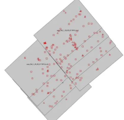
In this experiment, a block of four RGB images (Fig. 1) acquired with the Z/I DMC aerial camera was included. The image size was 3072x2048 pixels and because of approximately 530 meters flying height, the ground resolution of images was close to 22 cm. The ground resolution could have been improved by applying pan-sharpening process (Perco, 2005), but this was not included in this experiment.
Figure 1. Overview of the DMC (RGB) image block.
The orientations of images were solved beforehand by applying the aerial triangulation. Even if test data included only four images, the aerial triangulation was performed using a block of eight images. Fig. 2 illustrates how tie points and ground
control points located in the image planes. The set of four images was selected from the middle of the block.
Figure 2. The distribution of tie points and ground control points within the image block. Only four images from the middle of the block were included in the research.
ALS data was acquired in 2005 using the Optech ALTM 3100 scanner. Only a single ALS strip was applied and it covered quite well the stereo model areas of aerial images. The flying height was approximately 1000 m, resulting in a point density of 2-3 points/m2 (Fig. 3). The scanning angle was 24 degrees, the point repetition frequency 100 kHz, the scanning frequency 67 Hz, and the flying speed 75 m/s. For ensuring that ALS data sets were not at the same coordinate system as the images, ALS data was shifted and also slightly tilted and rotated.
Figure 3. A sample of Optech ALTM 3100 ALS data with a point density of 2-3 points/m2.
2.2 Reference materials
In order to check the correctness of relative orientations, six local reference areas were selected. Some ground control points were measured within each reference area using static GPS measurements ensuring the common coordinate system to all reference areas. Next, a total station was oriented using these ground control points. Through total station measurements, the coordinates of several spherical targets were solved. Finally, data from the Leica HDS6000 terrestrial laser scanner (TLS) was georeferenced using these spherical targets.
TLS data was further processed. Planes and free-form surfaces with varying orientations were extracted from ALS point clouds for each reference area. The accuracy of these reference surface measurements with TLS are assumed to be superior if compared with ALS data both in resolution and orientation. The aerial images were in the same coordinate system than the reference surfaces.
2.3 Methods
A relative orientation between ALS data and an aerial image block was solved using a variation of the interactive orientation method (Rönnholm et al., 2003). It was assumed that the block of aerial images was in the correct coordinate system after the aerial triangulation and the aim was to transform ALS data to the same coordinate system.
The interactive orientation method relies on operator’s visual interpretation and ability to change the exterior orientation parameters of a camera. Corrections of these parameters are done on the basis of visible misalignments detected when a laser scanning point cloud is superimposed into the image plane. Because the area under examination is larger than a single image, the strategy how the interactive orientation is applied was developed further from the original one. In this variation, an operator selects several small sample areas from different locations of the image block. Within each sample area an interactive relative orientation is performed using stereo vision. However, because the sample area is small, it cannot provide reliable information about rotation errors. Therefore, only shifts were applied to orientations. After the shifts were found for each sample area, the final shifts and rotations were solved using a least squares adjustment. In order to get point-like data in the least squares method, each sample area was represented with an original laser point chosen arbitrarily within the current test area, and its virtual tie point, which was calculated using the corresponding local shifts.
The interactive orientation method changes the exterior orientation parameters of a camera. Because the aim was to transform the laser point cloud and not images, the found orientation changes were inversed (Rönnholm et al., 2009).
Because the initial orientation was far from the correct one, the interactive orientation process was done twice. The first round was done very roughly, just to get data sets initially close to each others. In the second orientation round, the transformed laser point cloud from the first orientation was applied.
Because both the aerial images and data from the ground reference areas were at the same coordinate system, the transformed laser point clouds could be compared with planes and surfaces that were extracted from the reference areas. For this task, the distance between transformed ALS point clouds and reference planes and surfaces were minimized by applying the Iterative Closest Point (ICP) method implemented in Geomagic Qualify software. The comparison was done separately for each reference area.
3. RESULTS
The transformed ALS point clouds were compared with the reference at each of six reference areas. In the first case, six sample areas were selected and applied with the interactive orientation. These sample areas were not the same ones than the reference areas. The relative orientation mainly relied on ATFs.
The results from the comparison are listed in Table 1. In this case, the standard deviation of ∆Z describes also how well the
tilt and rotation between data sets have been defined. In Fig. 4, ALS data is superimposed onto a cross-eye stereo image pair illustrating how the point cloud is co-registered with image.
∆X (m) ∆Y (m) ∆Z (m)
Ref. area 1 0.305 0.134 -0.299
Ref. area 2 0.008 0.131 -0.739
Ref. area 3 0.221 0.102 -0.102
Ref. area 4 0.205 0.260 -0.306
Ref. area 5 0.164 0.135 -0.327
Ref. area 6 0.145 0.178 -0.389
Average 0.175 0.157 -0.360
STD 0.099 0.056 0.209
Table 1. The comparison of relatively oriented and transformed ALS data with the reference. In this case mostly ATFs, such as buildings, street lamps and fences, were applied.
Figure 4. A cross-eye stereo image pair of relatively oriented ALS data and aerial images.
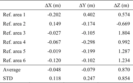
In the second case, only NTFs were included in the relative orientation. The process was similar with the case of ATFs, but the number of sample areas was increased to nine in order to increase reliability. The results from this experiment are visible in Table 2.
∆X (m) ∆Y (m) ∆Z (m)
Ref. area 1 -0.202 0.402 0.574
Ref. area 2 0.149 -0.174 -0.669
Ref. area 3 -0.027 -0.105 1.804
Ref. area 4 -0.067 -0.298 0.992
Ref. area 5 -0.019 -0.199 1.287
Ref. area 6 -0.120 -0.102 1.234
Average -0.048 -0.079 0.870
STD 0.118 0.247 0.854
Table 2. The comparison of relatively oriented and transformed ALS data with the reference. In this case NTFs, such as trees and ground surface, were applied during the orientation.
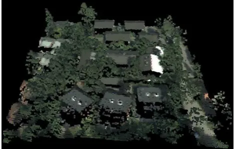
In Fig. 5, the oriented and transformed ALS point cloud is colorized by getting colour values from aerial images. In this ISPRS Annals of the Photogrammetry, Remote Sensing and Spatial Information Sciences, Volume I-3, 2012
case, NTFs were applied during the relative orientation. Fig. 6 illustrates the same data, but now a TIN surface model was created from the ALS points. The textures were interpolated from the colour information originally attached to the 3D ALS points.
Figure 5. The colorized ALS point cloud. The relative orientation was based on using only NTFs.
Figure 6. A TIN model with colour textures. The colour textures were interpolated from the colorized ALS point cloud illustrated in Fig. 5.
4. DISCUSSION
Even if using only NTFs appears to be more difficult in practice than using ATFs, XY shifts are solved well in both cases. The NTF case had six sample areas for solving a relative orientation whereas the ATF case included nine sample areas. If the effect of found averages of the planimetric errors is examined at the image plane, the error is clearly under one pixel anywhere in the images. The maximum error at reference areas causes the misalignment of less than two pixels.
Errors in the height component of the orientation parameters are significantly larger than the planimetric ones. Especially, using NTFs seems to cause difficulties to find correct height for an ALS point cloud. The effect is not as dramatic when using ATFs. Obviously, the height orientation error causes also misalignments on the image plane. The amount of misalignment varies according to the distance from the nadir point of the image. In the centre of the close-to-nadir images, the effect is
minimal. The maximum error is visible at the corners of the images.
Fig. 7 illustrates how much misalignment the detected average errors are causing on the image plane. The use of ATFs leaded to the average error that causes misalignment of less than one pixel on the image plane almost for the whole image. In the case of NTFs, the misalignment under one pixel can be found only from the central parts of the image. At the corners of the image, the misalignment is close to three pixels. In Fig. 8, a detail of the misalignment is illustrated in the case of NTFs. This detail includes a single ALS point hit from a lamp pole and is taken from the part of the image close to the upper edge of the image. The displacement of superimposed laser data at that area of the image seems to be close to 3 pixels, which corresponds to expectations. Such misalignments are not visible in those parts of the images that are highlighted with the green circle in Fig. 7.
Figure 7. Expected misalignment on the image plane after the registration due the detected average height error. In green areas misalignment is under one pixel, in yellow areas less than two pixels and in red areas under three pixels. The left image visualises the average height error of -0.36 m and the right image the average height error of 0.87 m.
Figure 8. A detail of the misalignment close to the edge of the image after the relative orientation using NTFs. In this case, laser observation (red dot) should hit to the top of a street lamp (white area). The majority of misalignment is caused by the orientation error along the direction of Z coordinate. The direction of the misalignment on the image plane is towards the nadir point of the image.
In reality, the height error is not behaving circularly, like presented in Fig. 7, but elliptically because of tilt errors. Fig. 7 was calculated using the average error without considering tilt errors just to give a general impression about the misalignments on the image plane. As can be seen from the results (Table 2), ISPRS Annals of the Photogrammetry, Remote Sensing and Spatial Information Sciences, Volume I-3, 2012
the standard deviation in the case of NTFs is relatively large. This indicates that inaccurate detection of heights at sample areas has caused also tilt errors. However, the rotation errors around the Z axis are not visible.
According to the results, the main error is included in the height direction. Therefore, we are able to examine the remaining error only in the direction of the Z coordinate axis. We made an additional experiment using NTFs, in which only the height parameter of the orientation was adjusted using a new sample area. In this time, the sample area was selected as close to the image edge as possible. The similar examination was repeated for both stereo pairs. As a result, the first case indicated 0.4087 m and the second case 1.1199 m height errors of orientations. This clearly confirms that some tilt errors exist. The average height error of the orientation calculated from these two height differences was 0.7643 m. If the average results in Table 2 were corrected with this additional result, only 0.1061 m average height error would remain. However, this examination would not correct the tilt problems.
Vegetation as a tie feature is not necessary stabile. In typical case, a wind is shifting tree canopies causing uncertainty to the orientation process. A stereoscopic examination reveals some of such shifts because there might become vertical parallaxes to stereo images. Vertical parallaxes disturb the stereo vision and therefore can be detected. However, in some cases the movement of canopies can lead changes only to horizontal parallaxes. In such cases, the height of the canopy is incorrect when examined stereoscopically. Therefore, high trees are not necessarily preferable tie features for a relative orientation. Instead, lower trees and bushes appear to be more robust ones. In addition, it is advantageous if the ground is visible within sample areas selected for local orientations.
The ground sample distance of images was 22 cm, which limits visibility of details. The lack of these details reduces the accuracy of stereo visibility. In addition, the base ratio of aerial images was approximately 0.3. The low base ratio of stereo images causes also negative effects to the height measurements. In our test case, the sample areas were selected on the basis where vegetation was available and where it appeared to be the most suitable for the interactive orientation. According to these criteria, the majority of the sample areas, in our case, were close to image centres and only few located close to the edges of the images. Our experiment suggests that it would be advantageous for detecting correct height if many of the sample areas locate close to the edges of the images.
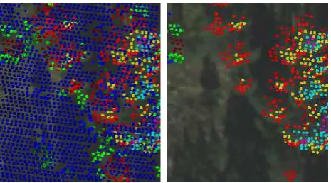
Different viewing angles of images compared to the acquisition direction of ALS data, as well as the ground hits of ALS data under the canopy, can cause difficulties to understand the stereo view. The reason for such phenomena is that ALS points can be behind solid objects that are visible in the stereo images. Therefore, it is advantageous to have tools that can hide temporarily those laser points that have height less than a given height threshold (Fig. 9). In addition, if only low vegetation or the ground surface is examined, correspondingly, hiding all ALS points higher to a threshold can improve the interpretability of the scene.
In the future, more research is needed in order to solve inaccuracies of the height estimation when using NTFs, and especially how tilt errors can be minimized. Also, more experiments are necessary to estimate how repeatable the current results are.
Figure 9. In some cases, hiding some of laser points can enchant interpretability. The left image illustrates all ALS points and the right image only points measured from the higher parts of the tree canopies.
5. CONCLUSIONS
We have solved a relative orientation between non-georeferenced ALS data and an oriented aerial image block using two types of tie features. In the first case, ATFs like buildings, street lamps, fences etc. were the basis of the relative orientation. In the second case, only NTFs like trees, bushes and ground surfaces were selected as tie features.
Despite of the selected tie feature type, relative orientations were solved applying the interactive orientation method with stereoscopic examination. This method uses unfiltered point clouds superimposed onto the images for an operator to detect and correct orientation errors. The final relative orientation was calculated using the orientation results from six to nine small sample areas.
The results were compared with the reference. The examination revealed that using ATFs for the orientation was reasonably successful. The average planimetric errors were under 0.18 m. However, the average height error of the orientation was approximately twice larger than planimetric errors. On the image plane, the effects of the average orientation errors caused misalignment less than one pixel for the most parts of the image.
As expected, the results when using NTFs were not as successful as with using ATFs. However, in our experiment, the average planimetric errors were only less than 0.08 m, which was actually smaller than in the case of ATFs. This result cannot be generalized before more comprehensive testing. The determination of correct heights, unfortunately, was not as successful causing detectable errors at the sample areas. Therefore, we detected relatively high average error in the direction of the Z coordinate axis. Inaccuracies of the heights caused also tilt errors. The errors in the heights cause misalignments on the image plane that are varying according to the distance to the nadir point of the image.
Afterwards, the height error was taken in a closer examination. It appeared that if only the height direction was taken account and sample area located close to the edge of the image, the amount of error could be detected. However, this examination did not solve tilt errors. Therefore, finding reliably tilt errors between data sets require further research. Most probably selecting more tie patches close to the edges of images, increasing image resolution and improving the base ratio would improve the orientation results. Even if our example, using ISPRS Annals of the Photogrammetry, Remote Sensing and Spatial Information Sciences, Volume I-3, 2012
NTFs during a relative orientation between ALS data and an image block, did not lead to perfect results, it revealed that there is a potential to find feasible tie features also in non-built environments.
Because vegetation is not as robust tie feature as artificial objects, the selection of tie patches should be chosen carefully. High vegetation tends to significantly move and change its shape in the wind and, therefore, can be unreliable if used as a tie feature. In many cases, lower vegetation and bare ground appears to be more feasible tie features than high vegetation.
6. REFERENCES
Csanyi, N. and Toth, C., 2007. Improvement of lidar data accuracy using lidar-specific ground targets. Photogrammetric Engineering & Remote Sensing, 73(4), pp. 385–396.
Heipke, C., Jacobsen K., and Wegmann H., 2002. Analysis of the results of the OEEPE test Integrated Sensor Orientation. Test Report and Workshop Proceedings, OEEPE Official Publication no 43, pp. 31–45.
Holmgren, J., Persson, Å. and Söderman, U., 2008. Species identification of individual trees by combining high resolution LiDAR data with multi-spectral images. International Journal of Remote Sensing, 29(5), pp. 1537–1552.
Honkavaara, E., Ilves, R., and Jaakkola, J., 2003. Practical results of GPS/IMU/camera-system calibration. Proceedings of International Workshop: Theory, Technology and Realities of Inertial/GPS Sensor Orientation, Castelldefels, Spain, 10 pages.
Huang, H., Gong, P., Cheng, X., Clinton, N., and Li, Z., 2009. Improving Measurement of Forest Structural Parameters by Co-Registering of High Resolution Aerial Imagery and Low Density LiDAR Data, Sensors, 9, pp. 1541–1558.
Kajuutti, K., Jokinen, O., Geist, T., and Pitkänen, T., 2007. Terrestrial Photography for Verification of Airborne Laser Scanner Data on Hintereisferner in Austria. Nordic Journal of Surveying and Real Estate Research 4(2), pp. 24–39.
Legat, K., Skaloud, J. and Schmidt, R., 2006. Reliability of Direct Georeferencing: A Case Study on Practical Problems and Solutions, Final Report on Phase 2. In EuroSDR Official Publication No 51, pp. 169–184.
Lowe, D. G., 2004. Distinctive Image Features from Scale-Invariant Keypoints. International Journal of Computer Vision, 60(2), pp. 91-110.
Packalén, P. and Maltamo, M., 2007. The k-MSN method for the prediction of species-specific stand attributes using airborne laser scanning and aerial photographs. Remote Sensing of Environment, 109(3), pp. 328–341.
Perco, R., 2005. Digital pansharpening versus full color film: A comparatice study. Institute for Computer Graphics and Vision, 6 pages, http://www.gtbi.net/export/sites/default/GTBiWeb/ soporte/descargas/DigitalPansharpeningVsColorFilm.pdf (accessed January 7, 2012)
Persson, Å., Holmgren, J., Söderman, U., and Olsson, H., 2004. Tree Species Classification of Individual Trees in Sweden by Combining High Resolution Laser Data with High Resolution
Near-Infrared Digital Images. International Archives of Photogrammetry, Remote Sensing and Spatial Information Sciences, 36(Part 8/W2), pp. 204–207.
Rönnholm, P., Hyyppä, H., Pöntinen, P., Haggrén, H., and Hyyppä, J., 2003. A Method for Interactive Orientation of Digital Images Using Backprojection of 3D Data, the Photogrammetric Journal of Finland, 18(2), pp. 58–69.
Rönnholm, P., Honkavaara, E., Litkey, P., Hyyppä, H., and Hyyppä, J., 2007. Integration of Laser Scanning and Photogrammetry. International Archives of Photogrammetry, Remote Sensing and Spatial Information Sciences, 36(3/W52): 355–362.
Rönnholm, P., Hyyppä, H., Hyyppä, J., and Haggrén, H., 2009. Orientation of Airborne Laser Scanning Point Clouds with Multi-View, Multi-Scale Image Blocks. Sensors, 9, pp. 6008– 6027.
Rönnholm, P., 2011. Registration Quality – Towards Integration of Laser Scanning and Photogrammetry. In EuroSDR Official Publication No 59, pp. 9–57.
Schenk, T. and Csathó, B., 2002. Fusion of LIDAR data and aerial imagery for a more complete surface description. International Archives of the Photogrammetry, Remote Sensing and Spatial Information Sciences, 34(3), pp. 310–317.
Vosselman, G., 2008. Analysis of planimetric accuracy of airborne laser scanning surveys. International Archives of Photogrammetry, Remote Sensing and Spatial Information Sciences, 37(Part 3A), pp. 99–104.
7. ACKNOWLEDGEMENTS
Authors would like to express their gratitude to the staff of the Finnish Geodetic Institute and also to EuroSDR (project Registration Quality - Towards Integration of Laser Scanning and Photogrammetry).