Staff Site Universitas Negeri Yogyakarta

(1)

Metal Machining

Theory and Applications

Thomas Childs

University of Leeds, UK

Katsuhiro Maekawa

Ibaraki University, Japan

Toshiyuki Obikawa

Tokyo Institute of Technology, Japan

Yasuo Yamane

Hiroshima University, Japan

A member of the Hodder Headline Group LONDON

Copublished in North, Central and South America by John Wiley & Sons Inc.

(2)

338 Euston Road, London NW1 3BH

http://www.arnoldpublishers.com

Copublished in North, Central and South America by John Wiley & Sons Inc., 605 Third Avenue,

New York, NY 10158–0012

All rights reserved. No part of this publication may be reproduced or transmitted in any form or by any means, electronically or mechanically, including photocopying, recording or any information storage or retrieval system, without either prior permission in writing from the publishers or a licence permitting restricted copying. In the United Kingdom such licences are issued by the Copyright Licensing Agency: 90 Tottenham Court Road,

London W1P 0LP.

Whilst the advice and information in this book are believed to be true and accurate at the date of going to press, neither the authors nor the publisher can accept any legal responsibility or liability for any errors or omissions

that may be made.

British Library Cataloguing in Publication Data A catalogue record for this book is available from the British Library

Library of Congress Cataloging-in-Publication Data A catalog record for this book is available from the Library of Congress

ISBN 0 340 69159 X ISBN 0 470 39245 2 (Wiley)

1 2 3 4 5 6 7 8 9 10

Commissioning Editor: Matthew Flynn Production Editor: James Rabson Production Controller: Iain McWilliams

Cover Design: Mouse Mat Design

Typeset in 10/12 pt Times by Cambrian Typesetters, Frimley, Surrey Printed and bound in Great Britain by Redwood Books Ltd.

(3)

Preface

Improved manufacturing productivity, over the last 50 years, has occurred in the area of machining through developments in the machining process, in machine tool technology and in manufacturing management. The subject of this book is the machining process itself, but placed in the wider context of manufacturing productivity. It is mainly concerned with how mechanical and materials engineering science can be applied to understand the process better and to support future improvements.

There have been other books in the English language that share these aims, from a vari-ety of viewpoints. Metal Cutting Principles by M. C. Shaw (1984, Oxford: Clarendon Press) is closest in spirit to the mechanical engineering focus of the present work, but there have been many developments since that was first published. Metal Cuttingby E. M. Trent (3rd edn, 1991, Oxford: Butterworth-Heinemann) is another major work, but written more from the point of view of a materials engineer than the current book’s perspective.

Fundamentals of Machining and Machine Toolsby G. Boothroyd and W. A. Knight (2nd edn, 1989, New York: Marcel Dekker) covers mechanical and production engineering perspectives at a similar level to this book. There is a book in Japanese,Modern Machining Theory by E. Usui (1990, Tokyo: Kyoritu-shuppan), that overlaps some parts of this volume. However, if this book,Metal Machining, can bear comparison with any of these, the present authors will be satisfied.

There are also more general introductory texts, such as Manufacturing Technology and Engineering by S. Kalpakjian (3rd edn, 1995, New York: Addison-Wesley) and

Introduction to Manufacturing Processes by J. A. Schey (2nd edn, 1987, New York: McGraw-Hill) and narrower more specialist ones such as Mechanics of Machiningby P. L. B. Oxley (1989, Chichester: Ellis Horwood) which this text might be regarded as complementing.

(8)

It is supposed that masters course readers will have encountered basic mechanical and materials principles before, but will not have had much experience of their application. A feature of the book is that many of these principles are revised and placed in the machin-ing context, to relate the material to earlier understandmachin-ing. Appendices are heavily used to meet this objective without interrupting the flow of material too much.

It is a belief of the authors that texts should be informative in practical as well as theo-retical detail. We hope that a reader who wants to know how much power will be needed to turn a common engineering alloy, or what cutting speed might be used, or what mater-ial properties might be appropriate for carrying out some reader-specific simulation, will have a reasonable chance either of finding the information in these pages or of finding a helpful reference for further searching.

The book is essentially organized in two parts. Chapters 1 to 5 cover basic material. Chapters 6 to 9 are more advanced. Chapter 1 is an introduction that places the process in its broader context of machine tool technology and manufacturing systems management. Chapter 2 covers the basic mechanical engineering of machining: mechanics, heat conduc-tion and tribology (fricconduc-tion, lubricaconduc-tion and wear). Chapters 3 and 4 focus on materials’ performance in machining, Chapter 5 describes experimental methods used in machining studies.

The core of the second part is numerical modelling of the machining process. Chapter 6 deals with mechanics developments up to the introduction of, and Chapters 7 and 8 with the development and application of, finite element methods in machining analysis. Chapter 9 is concerned with embedding process understanding into process control and optimiza-tion tools.

No book is written without external influences. We thank the following for their advice and help throughout our careers: in the UK, Professors D. Tabor, K. L. Johnson, P. B. Mellor and G . W. Rowe (the last two, sadly, deceased); in Japan, Professors E. Usui, T. Shirakashi and N. Narutaki; and Professor S. Ramalingam in the USA. More closely connected with this book, we also especially acknowledge many discussions with, and much experimental information given by, Professor T. Kitagawa of Kitami Institute of Technology, who might almost have been a co-author.

We also thank the companies Yasda Precision Tools KK, Okuma Corporation and Toyo Advanced Technologies for allowing the use of original photographs in Chapter 1, British Aerospace Airbus for providing the cover photograph, Mr G. Dean (Leeds University) for drafting many of the original line drawings and Mr K. Sekiya (Hiroshima University) for creating some of the figures in Chapter 4. One of us (it is obvious which one) thanks the British Council and Monbusho for enabling him to spend a 3 month period in Japan during the Summer of 1999: this, with the purchase of a laptop PC with money awarded by the Jacob Wallenberg Foundation (Royal Swedish Academy of Engineering Science), resulted in the final manuscript being less late than it otherwise would have been.

We must thank the publisher for allowing several deadlines to pass and our wives – Wendy, Yoko, Hiromi and Fukiko – and families for accepting the many working week-ends that were needed to complete this book.

(9)

1

Introduction

Machining (turning, milling, drilling) is the most widespread metal shaping process in mechanical manufacturing industry. Worldwide investment in metal-machining machine tools holds steady or continues to increase year by year, the only exception being in the worst of recessions. The wealth of nations can be judged by this investment. Figure 1.1 shows the annual expenditure on machine tools by each of the most successful countries – Germany, Japan and the USA. For each, it was between £1bn and £2bn (bn = 109_{) in the}

late 1970s. It fell abruptly in the world recession (the oil crisis) of 1981–82 and has now recovered to between £2bn and £3bn (all expressed in 1985 prices: £1 was then equivalent to 300¥ or $1.3). Figure 1.1 also shows similar trends (a growth over the last 20 years from

(10)

50% to 100% in annual expenditure) for the developed European Community countries. Only in the UK has there been a decline in investment. Over this period, investment in metal machining has remained at about three times the annual investment in metal form-ing machinery.

Investment has continued despite perceived threats to machining volume, such as the displacement of metal by plastics products in the consumer goods sector, and material wastefulness in the production of swarf (or chips) that has encouraged near-net (casting and forging) process substitution in the metal products sector. One reason is that metal machining is capable of high precision: part tolerances of 50mm and surface finishes of 1 mm are readily achievable (Figure 1.2(a)). Another reason is that it is very versatile: complicated free-form shapes with many features, over a large size range, can be made more cheaply, quickly and simply (at least in small numbers) by controlling the path of a standard cutting tool rather than by investing considerable time and cost in making a dedi-cated moulding, forming or die casting tool (besides, machining is needed to make the dies for moulding, forging and die casting processes).

One measure of a part’s complexity is the product of the number of its independent dimensions and the precision to which they must be made (Ashby, 1992). Figure 1.2(b) gives limits to the component size (weight units – a cube of steel of side 3 m weighs approximately 2 × 105kg) and complexity of machining and its competitive processes. Complexity is defined by

C = n log₂(l/Dl) (1.1)

where nis the number of the dimensions of the part and Dl/lis the average fractional preci-sion with which they are specified.

A third reason for the success of metal machining is that the need from competition to increase productivity, to hold market share and to find new markets, has led to large changes in machining practice. The changes have been of three types: advances in machine tools (machine technology), in the organization of machining (manufacturing systems) and in the cutting edges themselves (materials technology). Each new improvement in one area

Fig. 1.2 (a) Typical accuracy and finish and (b) complexity and size achievable by machining, forming and casting

(11)

throws pressure on to another. It is worthwhile briefly to review the evolution of these changes, from the introduction of numerical controlled machine tools in the late 1950s to the present day, in order to place in its wider context the special content of this book (the consideration of the chip forming process itself), which is at the heart of machining.

1.1 Machine tool technology

In the early 1970s a number of surveys were carried out on the productivity of machine shops in the UK, Europe and the USA (Figure 1.3). As far as the machine tools were concerned it was found that they were actually productive, removing metal, for only 10 to 20% of the time: different surveys, however, gave different values. For 40 to 60% of the time the machine tools were in use but not productively: i.e. they were being set up for manufacture, or being loaded and unloaded, or during manufacture tools were being moved and positioned for cutting but they were not removing metal. For 20 to 50% of the time they were totally unused – idle.

As far as work in progress was concerned, batches of components typically spent from 70 to 95% of their time inactive on the shop floor. So overwhelming was the clutter of partly finished work that a component requiring several different operations for its comple-tion, on different machine tools, might find these carried out at the rate of only one a week. From 10 to 20% of their time components were being positioned for machining and for only from 1 to 5% of the time was metal actually being removed.

(12)

1.1.1 Machine tool technology – mainly turning machines

From 1970 onwards, machine tools of new design started to be introduced in significant numbers into manufacturing industry, with the effect of greatly reducing the times for tool positioning and movement between cuts. These new, computer numerical control (CNC), designs stemmed directly from the development of numerically controlled (NC) machine tools in the 1950s. In traditional, mechanically controlled machine tools, for example the lathe in Figure 1.4, the coordination needed between the main rotary cutting motion of the workpiece and the feed motions of the tool is obtained by driving all motions from a single motor. The feed motions are obtained from the main motion via a gear box and a slender feed rod (or lead screw for thread cutting). With the exception of machines known as copy-ing machines (which derive their feed motion by followcopy-ing a copy of a shape to be made) only simple feed motions are obtainable: on a lathe, for example, these are in the axial and radial directions – to machine a radius on a lathe requires the use of a form tool. In addi-tion, the large amount of backlash in the mechanical chain requires time and a skilled oper-ator to set the tool at the right starting point for a particular cut.

In a CNC machine tool, all the motions are mechanically separate, each driven by its own motor (Figure 1.4) and each coordinated electronically (by computer) with the others. Not only are much more complicated feed motions possible, for example a combined radial and axial feed to create a radius or to take the shortest path between two points at different axial and radial positions, but the requirement of coordination has led to the development of much more precise, backlash-free ball-screw feed drives. This precise numerical control of feed motions, with the ability also to drive the tools quickly between cuts, together with other reductions in set-up times (to be considered in Section 1.2), has approximately halved machine tool non-productive cycle time, relative to its pre-1970 levels.

This halving of time is indicated in Figure 1.5(a) (Figure 1.5(b) is considered in Section 1.1.2). A further halving of non-productive cycle time has been possible from about 1980 onwards, with the spread throughout all manufacturing industry of new types of machine tools that have become called turning centres (related to lathes) and machining centres

(developed from milling machines). These new tools, first developed in the 1960s for mass production industry, individually can carry out operations that previously would have required several machine tools. For example, it is possible on a traditional lathe to present a variety of tools to the workpiece by mounting the tools on a turret. In a new turning centre, some of the tools may be power driven and the main power drive, usually used to rotate the workpiece in turning operations, may be used as a feed drive to enable milling and drilling as well as turning to be carried out on the one machine.

(13)

(14)

The increased versatility of machine tools (based on turning operations as an example) has been briefly considered: the freedom given by CNC to create more complicated feed motions, both by path and speed control; and the evolution of multi-function machine tools (centres). The cost penalty has just been mentioned. As part of the continuing scene setting for the conditions in which metal cutting is carried out, which will be combined with systems and materials technology considerations in Section 1.4, some broad machine tool mechanical design and cost considerations will now be introduced – still in the context of turning.

Figure 1.7 sketches a turning operation, in which, in one revolution of the bar, the tool moves an axial distance f (the feed distance) to reduce the bar radius by an amount d(the depth of cut). The figure also shows the cutting force F_cacting on the tool, the diameter D

at which the cutting is taking place and both the angular speed Wat which the bar rotates and the consequent linear speed V (in later chapters this will be called U_work) at the diam-eter D. Material is removed, in the form of chips, at the rate fdV. (More detail of cutting terminology is given in Chapter 2).

Fig. 1.5 Reductions from the levels shown in Figure 1.3 of (a) machine tool non-productive time and (b) work in progress idle time, due to better technology and organization

(15)

The torque Tand power Pthat the main drive motor must generate to support this turn-ing operation is, by elementary mechanics

T = F_c(D/2) ≡ (F_c*_fd₎₍_D_/2) _(1.2a)

P= F_cV ≡ (F_c*_fd₎_V_or_F

c*(fdV) (1.2b)

A new quantity F_c*_{has been introduced. It is the cutting force per unit area of removed} material. Called the specific cutting force, it depends to a first approximation mainly on the material being cut. Equation (1.2a) indicates that, for a constant area of cut fd, a turn-ing machine should be fitted with a motor with a torque capacity proportional to the largest diameter being cut. It is shown later that for any combination of work and tool there is a preferred linear cutting speed V. Equation (1.2b) suggests that for a constant area of cut the required motor power should be independent of diameter cut. Observing what motors, with their torque and power capacities, are fitted to production machine tools can give insight into what duties the machine tools are expected to perform; and what forces the cutting tools are expected to withstand. This is considered next.

Machine tool manufacturers’ catalogues show that turning machines are fitted with motors the torques and powers of which increase, respectively, with the square of and linearly with, the maximum work diameter. A typical catalogue specifies, among other things, the main motor power, the maximum rev/min at which the work rotates and the maximum diameter of work for which the machine is designed. Figure 1.8(a) plots the torque at maximum rev/min, obtained from P = WT, against maximum design diameter, both on a log scale, for a range of mechanically controlled and CNC centre lathes and chucking turning centres (as illustrated in Figures 1.4 and 1.6 respectively). Apart from two sets of data marked ‘t’, which are for lathes described as for training and which might be expected to be underdesigned relative to machines for production use, both the mechan-ical and CNC classes of machine show the same squared power law dependence of torque on maximum work diameter.

(16)

design specification that the maximum depth of cut dshould increase in proportion to the maximum work diameter D would, from equation (1.2a), give the observed squared power law.

Design cutting forces may be deduced from the torque/diameter relationship shown in Figure 1.8(a). For example the lowest torque of 10 N m in Figure 1.8(a) would be caused by a cutting force of 140 N at the diameter of 145 mm, while the upper limit around 50 N m would be caused by 270 N at 365 mm. Of course, a workpiece will not be machined only at its maximum diameter. The highest rotational speeds are, in fact, used at the small-est machined diameters (to maintain a high linear speed). If features were machined at one tenth maximum diameter, the 10 N m and 50 N m torques would be generated by cutting forces of 1.4 kN and 2.7 kN. The turning machines represented in Figure 1.8 are, in fact, designed to generate cutting forces up to 2 or 3 kN. These are the forces to which the cutting tools are exposed.

Figure 1.8(b) shows designed power is proportional to maximum work diameter, consistent with equation (1.2b) if d is proportional to D. Further, the CNC machines have motors up to twice as powerful as mechanically controlled machines for a given work diameter. The top rotational speeds of CNC machines tend to be twice those of mechani-cally controlled ones, for example 4000 to 5000 rev/min as opposed to 2000 to 2500 rev/min for maximum work diameters around 250 mm. It is tempting to speculate that this is part of a trend to higher productivity through higher cutting speeds (Section 1.4). This may be partly true, but there is also another reason – it is due to the different characteris-tics of the motors used in mechanically and CNC controlled machines. The main drive of a mechanically controlled lathe runs at constant speed, and different work rotational speeds are obtained through a gear box. Apart from gear box losses, the motor can deliver a constant power to the work, independent of work speed. A CNC main drive motor is a variable speed motor with, as illustrated in Figure 1.9, a power capacity that drops off at low rotation speeds, i.e. when turning at maximum bar diameter. To compensate for this, a motor with a higher power at high rotational speeds must be employed.

(17)

The cutting speeds Vat which the machine tools are expected to operate can be deduced from the available power and the expected cutting forces at high rotation speeds, i.e. at small cutting diameters. Continuing the example above, of a cutting force range of 1.4 kN to 2.7 kN; associating these with powers from 5 kW to 20 kW (Figure 1.8(b)), gives cutting speeds from 215 m/min to 450 m/min. It will be seen later (Section 1.3 and Chapter 3) that speeds in the range 100 to 1000 m/min are indeed practical for turning steels with cutting tools made from cemented carbides (tungsten and titanium carbides bonded by cobalt), which are the workhorse tools of today.

The dissipation of up to 5 to 20 kW through cutting tools results in them becoming very hot: 1000˚C is not unusual (this is justified later). For the tools to carry kN forces (or rather the associated stresses, approaching 1 GPa) at such temperatures requires high temperature strength. It is this that ultimately limits the productivity of cutting tools. Obsolete machine tools – from the 1960s and earlier – were provided with lower power motors (line A–A in Figure 1.8(b)) because they were designed for use with less produc-tive tools made from high speed steels, with a lower high-temperature strength than cemented carbides. Some modern machine tools, designed for use with ceramic tooling and higher cutting speeds, are being fitted with higher power motors (line B–B in Figure 1.8(b)).

These ‘facts of life’ of the turning process – forces up to 2 or 3 kN and cutting speeds up to 1000 m/min – are set by the material properties of the work and tool materials as well as the mechanics of the process. Later chapters will be devoted to the details of why these ‘facts of life’ are so. They, and the functional versatility considered earlier, determine the price of turning machine tools. Machines must have a sufficient bulk and mass to be stiff and stable when cutting the high speed rotating mass of the workpiece. Figure 1.10(a) shows, for the same machine tools as in Figure 1.8, how their masses increase in propor-tion to motor power (the maximum workpiece lengths are in the range 500 mm to 1 m; machine mass increases with workpiece length as well as diameter capacity). Mass turns out to be one practical measure of value in a machine tool, the other being versatility. Figure 1.10(b) shows the list price of machine tools (without tax) as a function of mass (the data were gathered in 1990).

(18)

Here and later in the Chapter, prices and costs have been collected in the UK, during the early 1990s. A decision has been made to leave the information in units of UK£, unad-justed for inflation. An approximate conversion to values in the USA may be made at UK£1 = US$1; and to values in Japan at UK£1 = ¥200. These are not general exchange rates but equivalent purchasing rates.

Mechanically controlled centre lathes vary in price from around £3000 to £30 000 as their mass increases from 500 kg to 5000 kg. Changing to CNC controlled main and feed drives (the 1970s development of Figure 1.5(a)) displaces the price/mass relation upwards by about £15 000, while the further development of increased functionality of turning centres displaces the relation upwards by at least a further £15 000 to £20 000. There is a wide range of turning centre prices per unit mass, reflecting the wide range of complexity that can be built in to such a machine in a manner tailored to suit the needs of the parts being machined on it. The more specialized the turning centre, the more productive it can be: the degree of investment that is worthwhile will depend on whether a manufacturer can keep it occupied. The most specialized tend to be used with robotic loading and unloading systems (see Section 1.2). The prices in Figure 1.10(b) do not include such external mater-ials handling devices.

1.1.2 Milling and drilling machines

(19)

time, investment in CNC machines was growing, equally spread between turning and milling. Post-1980, investment in mechanically controlled machines collapsed and that in CNC turning machines held steady, while CNC milling machine investment increased to the stage where it was twice that of turning machines. This increase was mainly due to the influence of machining centres.

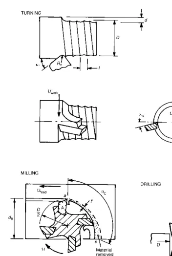
At first sight it is surprising that pre-1980 investment in substituting mechanically controlled for CNC-controlled milling machines equalled that for lathes, because there is less to be gained from reducing non-productive cycle times. The obvious difference between turning and milling processes is that, in turning, the main power is used to rotate an essentially cylindrical workpiece, with feed motions applied to the tool; whereas in milling the main power rotates a cutting tool, with the prismatic workpiece undergoing feed motions. Milling cutting tools have many cutting edges, and are more complicated than turning tools (Figure 1.12) and each edge cuts only intermittently. The cost of the tools makes it prudent to remove metal more slowly, and vibrations set up by the inter-mittent tool contacts reinforce this. The longer cutting times make the non-productive time less significant.

However, investment in milling machines in the pre-1980 period was not only in order to take advantage of the reduced non-productive time due to numerical control. A revolu-tion was taking place, not only in machine control but also in machine structure. When mechanical feed drives were replaced by individual ball-screw feed drives, it was found that the accuracy of the cut was no longer limited by the accuracy of the drive but by elas-tic deflection of the milling machine frame. The introduction of CNC control led directly to a mechanical redesign of milling machines in order to produce machines of higher stiff-ness and hence accuracy. Figure 1.13 compares the new type of design with the earlier one. In addition, the freedom to vary x–yfeed motions simultaneously to create curved feed paths opened up the possibilities for free-form shape generation by milling that existed before only with difficulty.

(20)

devised so that setting up of one part could be carried out while another part was being machined. In an extreme form, it was possible to pre-prepare parts on a carousel worktable, such that, with magazine tool changing, a milling machining centre could be loaded with enough work and tools to keep it running overnight without attention from an operator. These changes, much greater than the changes in the development of turning centres from lathes, explain the greater investment in milling than turning in the post-1980 period as shown in Figure 1.11. Figure 1.14 shows an example of a new design of machine with a tiltable spin-dle and interchangeable worktables. Figure 1.15 shows a detail of a tool change magazine.

As far as process mechanics is concerned, equations (1.2) for torque and power can be applied to milling if D is interpreted as the diameter of the cutting tool and fdVremains the volume removal rate. However, torque and power are not limited by workpiece stiff-ness. It is the stiffness or strength of the cutter spindle that is important. The polar second moment of area J of a shaft is proportional to D to the fourth power, and surface stress in a shaft varies as TD/J. The torque T to create a given surface stress thus increases as D3_. The torque to create a given angular twist of the spindle also increases as D3_{, if spindle} length increases in proportion to D. A torque increases as D3_{if cutting force increases as}

(21)

In Figures 1.16(a) and (b) the capacity of a milling machine is measured by its cross-traverse capacity. This defines maximum workpiece size in a similar manner to defining the capacity of a turning centre by maximum work diameter (Figure 1.8). Figures 1.16(a) and (b) show that torque and power increase as cross-traverse cubed and squared respec-tively. An assumption that machines are designed to accommodate larger diameter cutters in proportion to workpiece size yields the D3_and_D2 _{relations derived in the previous} paragraph.

(22)

If Figure 1.16(b) is compared with Figure 1.8(b) it is seen that for given workpiece size (cross-traverse or work diameter) a milling machine is likely to have from one fifth to one half the power capacity of a turning machine, depending on size. This means that milling machines are designed for lower material removal rates than are turning machines, for a given size of work. Figure 1.16(c), when compared with Figure 1.10(a), shows that milling machines are up to twice as massive per unit power as turning machines, reflecting the greater need for rigidity of the (more prone to vibration) milling process. Figure 1.16(d), admittedly based on a rather small amount of data, shows little difference in price between milling and turning machines when compared on a mass basis. Combining all these rela-tionships, the price of a milling machine is about 2/3 that of a turning machine for a 200 mm size workpiece but rises to 1.5 times the price for 1000 mm size workpieces. The consequences for economic machining of these different capital costs, as well as the differ-ent removal rate capacities that stem from the differdiffer-ent machine powers, are returned to in Section 1.4.

(23)

milling machines: there is less tendency for vibration and the axial thrust causes less distortion than the side thrusts that occur on a milling cutter. The prices of drilling machines are negligible compared with milling or turning. On the other hand, the low power availability implies a much lower material removal rate capacity. It is perhaps a saving grace of the drilling process that not much material is removed by it. This too is taken up in Section 1.4.

1.2 Manufacturing systems

The attack on non-productive cycle times described in the previous section has resulted in machine tools capable of higher productivity, but they are also more expensive. If they had been available in the late 1960s, they would have been totally uneconomic as the manu-facturing organization was not in place to keep them occupied. The flow of work in progress was not effectively controlled, so that batches of components could remain in a factory totally idle for up to 95% of the time, and even the poorly productive machines that were then common were idle for up to 50% of the time (Figure 1.3). Manufacturing tech-nology has, in fact, evolved hand in hand with manufacturing system organization, some-times one pushing and the other pulling, somesome-times vice versa.

(24)

In the late 1960s there were two standard forms of organizing the machine tools in a machine shop. At one extreme, suitable for the dedicated production of one item in long runs – for example as might occur in converting sheet metal, steel bar, casting metal, paint and plastics parts into a car (Figure 1.17) – machine tools were laid out in flow lines or transfer lines. One machine tool followed another in the order in which operations were performed on the product. Such dedication allowed productivity to be gained at the price of flexibility. It was very costly to create the line and to change it to accommodate any change in manufacturing requirements.

(25)

manufactured by carrying them from area to area as dictated by the ordering of their oper-ations. It resulted in tortuous paths and huge amounts of materials handling – a part could travel several kilometres during its manufacture (Figure 1.18). It is to these circumstances that the survey results in Figure 1.3 apply.

(26)

appropriate for different mixes of part variety and quantity (Figure 1.19). If a manufac-turer’s spectrum of parts is of the order of thousands made in small batches, less than 10 to 20 or even one at a time, then planning improved materials handling strategies is prob-ably not worthwhile. The large amounts of materials handling associated with job shop or process oriented manufacture cannot be avoided. Investment in highly productive machine tools is hard to justify. Such a manufacturer, for example a general engineering workshop tendering for sub-contract prototype work from larger companies, may still have some mechanically controlled machines, although the higher quality and accuracy attainable from CNC control will have forced investment in basic CNC machines. (As a matter of fact, the large jobbing shop is becoming obsolete. Its low productivity cannot support a large overhead, and smaller, perhaps family based, companies are emerging, offering specialist skills over a narrow manufacturing front.)

Fig. 1.18 Materials transfers in a jobbing shop environment (after Boothroyd and Knight, 1989)

(27)

If part variety reduces, perhaps to the order of hundreds, and batch size increases, again to the order of hundreds, it begins to pay to organize groups or cells of machine tools to reduce materials handling (Figure 1.20). The classification of parts to reduce, in effect, their variety from the manufacturing point of view is one aspect of the discipline of Group Technology. Almost certainly the machine tools in a cell will be CNC, and perhaps the programming of the machines will be from a central cell processor (direct numerical control or DNC). A low level of investment in turning or machining centre type tools may be justified, but it is unlikely that automatic materials handling outside the machine tools (robotics or automated guided vehicles – AGVs) will be justifiable. Cell-oriented manu-facture is typically found in companies that own products that are components of larger assemblies, for example gear box, brakes or coupling manufacturers.

As part variety reduces further and batch size increases, say to tens and thousands respectively, the organization known as a flexible manufacturing system becomes justifi-able. Heavy use can be justified of turning and/or machining centres and automatic handling between machine tools. Flexible manufacturing systems are typically found in companies manufacturing high value-added products, who are further up the supply chain than the component manufacturers for whom cell-oriented manufacture is the answer. Examples are manufacturers of ranges of robots, or the manufacturers of ranges of machine tools themselves (Figure 1.21). (Figure 1.19 also identifies a flexible transfer line layout – this could describe, for example, an automotive transfer line modified to cope with several variants of cars.)

The work in progress idle time (Figure 1.3) that has been the driver for the development of manufacturing systems practice has been reduced typically by half in circumstances suitable for cell-oriented manufacture and by a further half again in flexible manufactur-ing systems (Figure 1.5(b)), which is in balance with the increased capacity to remove metal of the machine tools themselves (Figure 1.5(a)).

1.3 Materials technology

(28)

properties of these cutting edges that limit the material removal rates that can be achieved by them; how they are held in the machine tool, which determines how quickly they may be changed when they are worn out; and their price.

1.3.1 Cutting tool material properties

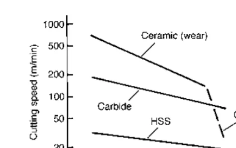
The main treatment of materials for cutting tools is presented in Chapter 3. As a summary, typical high temperature hardnesses of the main classes of cutting tool materials (high speed steels, cemented carbides and cermets, and alumina and silicon nitride ceramics; diamond and cubic boron nitride materials are introduced in Chapter 3) are shown in Figure 1.22. The temperatures that have been measured on tool rake faces during turning various work materials at a feed of 0.25 mm are shown in Figure 1.23. If the work mater-ial removal rate that can be achieved by a cutting tool is limited by the requirement that its hardness must be maintained above some critical level (to prevent it collapsing under the stresses caused by contact with the work), it is clear that carbide tools will be more produc-tive than high speed steel tools; and ceramic tools may, in some circumstances, be more productive than carbides (for ceramics, toughness, not hardness, can limit their use). Also, copper alloys will be able to be machined more rapidly than ferrous alloys and than tita-nium alloys.

(29)

0.25 mm with high speed steel, a cemented carbide and an alumina ceramic tool (the data for the ceramic tool show a fracture (chipping) range). Over the straight line regions (on a log-log basis), and with Tin minutes and Vin m/min

for high speed steel VT0.15 _{= 30} _(1.3a)

for cemented carbide VT0.25 _{= 150} _(1.3b)

for alumina ceramic VT0.45 _{= 500} _(1.3c)

These representative values will be used in the economic considerations of machining in Section 1.4. A more detailed consideration of life laws is presented in Chapter 4. The constants n and C in the life laws typically vary with feed as well as cutting speed; they also depend on the end of life criterion, reducing as the amount of wear that is regarded as allow-able reduces. At the level of this introductory chapter treatment, it is not straightforward to discuss how the constants in equations (1.3) may differ between turning, milling and drilling practice. It will be assumed that they are not influenced by the machining process. Any important consequences of this assumption will be pointed out where relevant. Fig. 1.22 The hardness of cutting tool materials as a function of temperature

(30)

1.3.2 Cutting tool costs

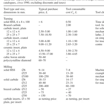
Apart from tool lifetime, the replacement cost of a worn tool (consumable cost) and the time to replace a worn-out tool are important in machining economics. Machining economics will be considered in Section 1.4. Some different forms of cutting tool have already been illustrated in Figure 1.12. High speed steel (HSS) tools were traditionally ground from solid blocks. Some cemented carbide tools are also ground from solid, but the cost of cemented carbide often makes inserts brazed to tool steel a cheaper alternative. Most recently, disposable, indexable, insert tooling has been introduced, replacing the cost and time of brazing by the cheaper and quicker mechanical fixing of a cutting edge in a holder. Disposable inserts are the only form in which ceramic tools are used, are the domi-nant form for cemented carbides and are also becoming more common for high speed steel tools. Typical costs associated with different sizes of these tools, in forms used for turning, milling and drilling, are listed in Table 1.1.

There are three sorts of information in Table 1.1. The second column gives purchase prices. It is the third column, of more importance to the economics of machining, that gives the tool consumable costs. A tool may be reconditioned several times before it is thrown away. The consumable cost C_t is the initial price of the tool, plus all the reconditioning costs, divided by the number of times it is reconditioned. It is less than the purchase price (if it were more, reconditioning would be pointless). For example, if a solid or brazed tool can be reground ten times during its life, the consumable cost is one tenth the purchase price plus the cost of regrinding. If an indexable turning insert has four cutting edges (for example, if it is a square insert), the consumable cost is one quarter the purchase price plus the cost of resetting the insert in its holder (assumed to be done with the holder removed from the machine tool). If a milling tool is of the insert type, say with ten inserts in a holder, its consumable cost will be ten times that of a single insert.

[image:30.595.129.366.63.212.2]

(31)

cutter diameter; and that drilling is similar to milling with respect to regrind conditions. There is clearly great scope for these costs to vary. The interested reader could, by the meth-ods of Section 1.4, test how strongly these assumptions influence the costs of machining.

To extend the range of Table 1.1, some data are also given for the price and consumable costs of coated carbide, cubic boron nitride (CBN) and polycrystalline diamond (PCD) inserts. Coated carbides (carbides with thin coatings, usually of titanium nitride, titanium carbide or alumina) are widely used to increase tool wear resistance particularly in finish-ing operations; CBN and PCD tools have special roles for machinfinish-ing hardened steels (CBN) and high speed machining of aluminium alloys (PCD), but will not be considered further in this chapter.

[image:31.595.61.420.80.436.2]

Finally, Table 1.1 also lists typical times to replace and set tool holders in the machine tool. This tool change time is associated with non-productive time (Figure 1.3) for most machine tools but, for machining centres fitted with tool magazines, tool replacement in the magazine can be carried out while the machine is removing metal. For such centres, Table 1.1 Typical purchase price, consumable cost and change time for a range of cutting tools (prices from UK catalogues,circa1990, excluding discounts and taxes)

Tool type and size, Typical purchase Tool consumable

dimensions in mm. price, £. cost C_t, £. Tool change time t_ct, min.

Turning

solid HSS, 6 x 8 x 100 ≈6 0.50 Time depends on machine

Brazed carbide – 2.00 tool: for example 5 min.

carbide insert, plain for solid tooling on

12 x 12 x 4 2.50–5.00 1.00–1.60 mechanical or simple CNC

25 x 25 x 7 7.50–10.50 2.30–3.00 lathe; 2 min for insert tooling

carbide insert, coated on simple CNC lathe; 1 min

12 x 12 x 4 3.00–6.00 1.10–1.90 for insert tooling on turning

25 x 25 x 7 9.00–11.20 2.65–3.20 centre

ceramic insert, plain

12 x 12 x 4 4.50–9.00 1.50–2.70

25 x 25 x 7 13.50–17.00 3.80–4.65

cubic boron nitride 50–60 –

polycrystalline diamond 60–70 –

Milling

solid HSS ∅6 9–14 7–8 Machine dependent, for

∅25 30–60 13–20 example 10 min for

∅100 100–250 30–60 mechanical machine; 5 min

solid carbide ∅6 18–33 14–17 for simple CNC mill; 2 min

∅12 40–80 23–31 for machining centre

∅25 200–400 60–100

brazed carbide∅12 ≈50 ≈27

∅25 ≈75 ≈40

∅50 ≈150 ≈70

carbide inserts,∅> 50 as turning price as turning, per insert plain, per insert

Drilling –

solid HSS ∅3 ≈1 – 3 ≈1.00

∅6 ≈1.5 – 5 ≈1.25

∅12 ≈3 – 8 ≈1.50

solid carbide ∅3 ≈7 ≈3.00

∅6 ≈15 ≈3.75

(32)

non-productive tool change time, associated with exchanging the tool between the maga-zine and the main drive spindle, can be as low as 3 s to 10 s. Care must be taken to inter-pret appropriately the replacement times in Table 1.1.

1.4 Economic optimization of machining

The influences of machine tool technology, manufacturing systems management and materials technology on the cost of machining can now be considered. The purpose is not to develop detailed recommendations for best practice but to show how these three factors have interacted to create a flow of improvement from the 1970s to the present day, and to look forward to the future. In order to discuss absolute costs and times as well as trends, the machining from tube stock of the flanged shaft shown in Figure 1.6 will be taken as an example. Dimensions are given in Figure 1.25. The part is created by turning the external diameter, milling the keyway, and drilling four holes. The turning operation will be consid-ered first.

1.4.1 Turning process manufacturing times

The total time,t_total, to machine a part by turning has three contributions: the time t_load

taken to load and unload the part to and from a machine tool; the time t_activein the machine tool; and a contribution to the time taken to change the turning tool when its edge is worn out.t_activeis longer than the actual machining time t_machbecause the tool spends some time moving and being positioned between cuts. t_activemay be written t_mach/f_mach, where f_mach

is the fraction of the time spent in removing metal. If machining N parts results in the tool edge being worn out, the tool change time t_ctallocated to machining one part is t_ct/N. Thus

(33)

t_mach t_ct

t_total= t_load+ ——— + — (1.4)

f_mach N

It is easy to show that as the cutting speed of a process is increased,t_totalpasses through a minimum value. This is because, although the machining time decreases as speed increases, tools wear out faster and N also decreases. Suppose the volume of material to be removed by turning is written V_vol, then

V_vol

t_mach= —— (1.5)

fdV

The machining time for N parts is N times this. If the time for N parts is equated to the tool life time T in equation (1.3) (generalized to VTn = C),Nmay be written in terms of nand

C,f,d,V_voland V, as

fdC1/n

N= ————— (1.6)

V_volV(1–n)/n

Substituting equations (1.5) and (1.6) into equation (1.4):

1 V_vol V_volV(1–n)/n

t_total= t_load+ ——— —— + —————— t_ct (1.7)

f_mach fdV fdC1/n

Equation (1.7) has been applied to the part in Figure 1.25, as an example, to show how the time to reduce the diameter of the tube stock from 100 mm to 50 mm, over the length of 50 mm, depends on both what tool material (the influence of n and C) and how advanced a machine technology is being used (the influence of f_machand t_ct). In this exam-ple,V_volis 2.95 ×105mm3. It is supposed that turning is carried out at a feed and depth of cut of 0.25 mm and 4 mm respectively, and that t_loadis 1 min (an appropriate value for a component of this size, according to Boothroyd and Knight, 1989). Times have been esti-mated for high speed steel, cemented carbide and an alumina ceramic tool material, in solid, brazed or insert form, used in mechanical or simple CNC lathes or in machining centres. nand Cvalues have been taken from equation (1.3). The f_machand t_ctvalues are listed in Table 1.2. The variation of f_machwith machine tool development has been based on active non-productive time changes shown in Figure 1.5(a). t_ctvalues for solid or brazed and insert cutting tools have been taken from Table 1.1. Results are shown in Figure 1.26. Figure 1.26 shows the major influence of tool material on minimum manufacturing

Table 1.2Values of f_machand t_ct, min, depending on manufacturing technology Tool form Machine tool development

Mechanical Simple CNC Turning centre

Solid or brazed f_mach= 0.45; t_ct= 5 f_mach= 0.65; t_ct= 5

(34)

time: from around 30 min to 40 min for high speed steel, to 5 min to 8 min for cemented carbide, to around 3 min for alumina ceramic. The time saving comes from the higher cutting speeds allowed by each improvement of tool material, from 20 m/min for high speed steel, to around 100 m/min for carbide, to around 300 m/min for the ceramic tooling.

For each tool material, the more advanced the manufacturing technology, the shorter the time. Changing from mechanical to CNC control reduces minimum time for the high speed steel tool case from 40 min to 30 min. Changing from brazed to insert carbide with a simple CNC machine tool reduces minimum time from 8 min to 6.5 min, while using insert tooling in a machining centre reduces the time to 5 min. Only for the ceramic tooling are the times relatively insensitive to technology: this is because, in this example, machining times are so small that the assumed work load/unload time is starting to dominate.

It is always necessary to check whether the machine tool on which it is planned to make a part is powerful enough to achieve the desired cutting speed at the planned feed and depth of cut. Table 1.3 gives typical specific cutting forces for machining a range of mater-ials. For the present engineering steel example, an appropriate value might be 2.5 GPa. Then, from equation 1.2(b), for fd= 1 mm2_{, a power of 1 kW is needed at a cutting speed} of 25 m/min (for HSS), 5 kW is needed at 120 m/min (for cemented carbide) and 15 kW Fig. 1.26 The influence on manufacturing time of cutting speed, tool material (high speed steel/carbide/ceramic) and manufacturing technology (solid/brazed/insert tooling in a mechanical/simple CNC/turning centre machine tool) for turning the part in Figure 1.25

Table 1.3Typical specific cutting force for a range of engineering materials

Material F*

c, GPa Material F*c, GPa

Aluminium alloys 0.5–1.0 Carbon steels 2.0–3.0

Copper alloys 1.0–2.0 Alloy steels 2.0–5.0

(35)

is needed around 400 m/min (for ceramic tooling). These values are in line with supplied machine tool powers for the 100 mm diameter workpiece (Figure 1.8).

1.4.2 Turning process costs

Even if machining time is reduced by advanced manufacturing technology, the cost may not be reduced: advanced technology is expensive. The cost of manufacture C_pis made up of two parts: the time cost of using the machine tool and the cost C_tof consuming cutting edges. The time cost itself comprises two parts: the charge rate M_tto recover the purchase cost of the machine tool and the labour charge rate M_wfor operating it. To continue the turning example of the previous section:

V_volV(1–n)/n

C_p= (M_t+ M_w)t_total+ ————— C_t (1.8)

fdC1/n

The machine charge rate

M_tis the rate that must be charged to recover the total capital cost C_mof investing in the machine tool, over some number of years Y. There are many ways of estimating it (Dieter, 1991). One simple way, leading to equation (1.9), recognizes that, in addition to the initial purchase price C_i, there is an annual cost of lost opportunity from not lending C_ito some-one else, or of paying the interest on C_iif it has been borrowed. This may be expressed as a fraction f_i of the purchase price. f_i typically rises as the inflation rate of an economy increases. There is also an annual maintenance cost and the cost of power, lighting, heat-ing, etc associated with using the machine, that may also be expressed as a fraction,f_m, of the purchase price. Thus

C_m= C_i(1 + [f_i+ f_m]Y) (1.9)

Earnings to set against the cost come from manufacturing parts. If the machine is active for a fraction f_oof n_s8-hour shifts a day (n_s= 1, 2 or 3), 250 days a year, the cost rate M_t for earnings to equal costs is, in cost per min

C_i 1

M_t= —————

[

— + (f_i+ f_m)

]

(1.10) 120 000f_on_s Y

(36)

The labour charge rate

M_wis more than the machine operator’s wage rate or salary. It includes social costs such as insurance and pension costs as a fraction f_sof wages. Furthermore, a company must pay all its staff, not only its machine operators. M_wshould be inflated by the ratio,r_w, of the total wages bill to that of the wages of all the machine operator (productive) staff. If a worker’s annual wage is C_a, and an 8-hour day is worked, 220 days a year, the labour cost per minute is

C_a

M_w= ———— (1 + f_s)r_w (1.11)

110 000

Table 1.5 gives some values for C_a = £15 000/year, typical of a developed economy country, and f_s= 0.25. r_wvaries with the level of automation in a company. Historically, for a labour intensive manufacturing company, it may be as low as 1.2, but for highly auto-mated manufacturers, such as those who operate transfer and FMS manufacturing systems, it has risen to 2.0.

Example machining costs

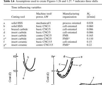
Equation (1.8) is now applied to estimating the machining costs associated with the times of Figure 1.26, under a range of manufacturing organization assumptions that lead to different cost rates, as just discussed. These are summarized in Table 1.6. Machine tools have been selected of sufficient power for the type of tool material they use. M_tvalues have been extracted from Table 1.4, depending on the machine cost and the types of manufac-turing organization of the examples. M_wvalues come from Table 1.5. Tool consumable costs are taken from Table 1.1. Two-shift operation has been assumed unless otherwise indicated. Results are shown in Figure 1.27.

Table 1.4Cost rates,M_t, £/min, for turning machines for a range of circumstances

Machine type C_i, £ Manufacturing system

Process-oriented Cell-oriented FMS

f_o= 0.5 f_o= 0.75; f_o= 0.85;

n_s= 2 n_s= 2 n_s= 2 n_s= 3

Mechanical 1 kW 6000 0.028

Simple CNC 1 kW 20000 0.092 0.060

5 kW 28000 0.13 0.086

15 kW 50000 0.23 0.15

Turning centre 5 kW 60000 0.18 0.16 0.11

15 kW 120000 0.37 0.33 0.22

Table 1.5 Range of labour rates, £/min, in high wage manufacturing industry Manufacturing organization

Labour intensive Intermediate Highly automated

(37)

Figure 1.27 shows that, as with time, minimum costs reduce as tool type changes from high speed steel to carbide to ceramic. However, the cost is only halved in changing from high speed steel to ceramic tooling, although the time is reduced about 10-fold. This is because of the increasing costs of the machine tools required to work at the increasing speeds appropriate to the changed tool materials.

The costs associated with the cemented carbide insert tooling, curves d, e and e* are particularly illuminating. In this case, it is marginally more expensive to produce parts on a turning centre working at FMS efficiency than on a simple (basic) CNC machine work-ing at a cell-oriented level of efficiency, at least if the FMS organization is used only two shifts per day (comparing curves d and e). To justify the FMS investment requires three shift per day (curve e*).

[image:37.595.61.420.74.373.2]

To the right-hand side of Figure 1.27 has been added a scale of machining cost per kg of metal removed, for the carbide and ceramic tools. The low alloy steel of this example probably costs around £0.8/kg to purchase. Machining costs are large compared with materials costs. When it is planned to remove a large proportion of material by machining, paying more for the material in exchange for better machinability (less tool wear) can often be justified.

Table 1.6Assumptions used to create Figures 1.26 and 1.27. * indicates three shifts Time influencing variables

Machine tool/ Manufacturing M_t, M_w, C_t,

Cutting tool power, kW organization [£/min] [£/min] [£]

a solid HSS mechanical/1 process oriented 0.028 0.20 0.50

b solid HSS basic CNC/1 cell-oriented 0.060 0.27 0.50

c brazed carbide basic CNC/5 cell-oriented 0.086 0.27 2.00

d insert carbide basic CNC/5 cell-oriented 0.086 0.27 1.50

e insert carbide centre CNC/5 FMS 0.165 0.34 1.50

e* insert carbide centre CNC/5 FMS* 0.110 0.34 1.50

f insert ceramic basic CNC/15 cell-oriented 0.15 0.27 2.50

g* insert ceramic centre CNC/15 FMS* 0.22 0.34 2.50

(38)

Up to this point, only a single machining operation – turning – has been considered. In most cases, including the example of Figure 1.25 on which the present discussion is based, multiple operations are carried out. It is only then, as will now be considered, that the orga-nizational gains of cell-oriented and FMS organization bring real benefit.

1.4.3 Milling and drilling times and costs

Equations (1.7) and (1.8) for machining time and cost of a turning operation can be applied to milling if two modifications are made. A milling cutter differs from a turning tool in that it has more than one cutting edge, and each removes metal only intermittently. More than one cutting edge results in each doing less work relative to a turning tool in removing a given volume of metal. The intermittent contact results in a longer time to remove a given volume for the same tool loading as in turning. Suppose that a milling cutter has n_ccutting edges but each is in contact with the work for only a fraction aof the time (for example a = 0.5 for the 180˚ contact involved in end milling the keyway in the example of Figure 1.25). The tool change time term of equation (1.7) will change inversely as n_c, other things being equal. The metal removal time will change inversely as (an_c):

1 V_vol V_volV(1–n)/n

t_total= t_load+ —— ——— + ————— t_ct (1.12)

f_mach an_cfdV n_cfdC1/n

Cost will be influenced indirectly through the changed total time and also by the same modification to the tool consumable cost term as to the tool change time term:

V_volV(1–n)/n

C_p= (M_t+ M_w)t_total+ ————— C_t (1.13)

n_cfdC1/n

[image:38.595.159.341.273.304.2]

For a given specific cutting force, the size of the average cutting force is proportional to the group [an_cfd]. Suppose the machining times and costs in milling are compared with those in turning on the basis of the same average cutting force for each – that is to say, for the same material removal rate – first of all, for machining the keyway in the example of Figure 1.25; and then suppose the major turning operations considered in Figures 1.26 and 1.27 were to be replaced by milling.

In each case, suppose the milling operation is carried out by a four-fluted solid carbide end mill (n_c= 4) of 6 mm diameter, at a level of organization typical of cell-oriented manu-facture: the appropriate turning time and cost comparison is then shown by results ‘brazed/CNC’ in Figure 1.26 and ‘c’ in Figure 1.27.

(39)

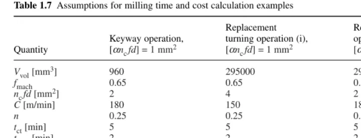
If milling were carried out at the same average force level as turning, peak forces would exceed turning forces. For this reason, it is usual to reduce the average force level in milling. Table 1.7 also lists (in its last column) coefficients assumed in the calculation of times and costs for the turning replacement operation with average force reduced to half the value in turning.

Application of equations (1.12) and (1.13) simply shows that for such a small volume of material removal as is represented by the keyway, time and cost is dominated by the work loading and unloading time. Of the total time of 2.03 min, calculated near minimum time conditions, only 0.03 min is machining time. At a cost of £0.36/min, this translates to only £0.011. Although it is a small absolute amount, it is the equivalent of £1.53/kg of material removed. This is similar to the cost per weight rate for carbide tools in turning (Figure 1.27).

[image:39.595.60.420.73.210.2]

In the case of the replacement turning operation, Figure 1.28 compares the two sets of data that result from the two average force assumptions with the results for turning with

Table 1.7Assumptions for milling time and cost calculation examples

Replacement Replacement turning

Keyway operation, turning operation (i), operation (ii), Quantity [αn_cfd] = 1 mm2 _[_α_n

cfd] = 1 mm2 [αncfd] = 0.5 mm2

V_vol[mm3_] ₉₆₀ ₂₉₅₀₀₀ ₂₉₅₀₀₀

f_mach 0.65 0.65 0.65

n_cfd[mm2_] ₂ ₄ ₂

C[m/min] 180 150 180

n 0.25 0.25 0.25

t_ct[min] 5 5 5

t_load[min] 2 2 2

M_m[£/min] 0.092 0.092 0.092

M_w[£/min] 0.27 0.27 0.27

C_t[£] 15 15 15

[image:39.595.78.404.83.402.2]

(40)

a brazed carbide tool. When milling at the same average force level as in turning (curves ‘i’), the minimum production time is less than in turning, but the mimimum cost is greater. This is because fewer tool changes are needed (minimum time), but these fewer changes cost more: the milling tool consumable cost is much greater than that of a turn-ing tool. However, if the average millturn-ing force is reduced to keep the peak force in bounds, both the minimum time and minimum cost are significantly increased (curves ‘ii’). The intermittent nature of milling commonly makes it inherently less productive and more costly than turning.

The drilling process is intermediate between turning and milling, in so far as it involves more than one cutting edge, but each edge is continuously removing metal. Equations (1.12) and (1.13) can be used with a= 1. For the example concerned, the time and cost of removing material by drilling is negligible. It is the loading and unloading time and cost that dominates. It is for manufacturing parts such as the flanged shaft of Figure 1.25 that turning centres come into their own. There is no additional set-up time for the drilling operation (nor for the keyway milling operation).

1.5 A forward look

The previous four sections have attempted briefly to capture some of the main strands of technology, management, materials and economic factors that are driving forward metal machining practice and setting challenges for further developments. Any reader who has prior knowledge of the subject will recognize that many liberties have been taken. In the area of machining practice, no distinction has been made between rough and finish cutting. Only passing acknowledgement has been made to the fact that tool life varies with more than cutting speed. All discussion has been in terms of engineering steel workpieces, while other classes of materials such as nickel-based, titanium-based and abrasive silicon-aluminium alloys, have different machining characteristics. These and more will be considered in later chapters of this book.

Nevertheless, some clear conclusions can be drawn that guide development of machining practice. The selection of optimum cutting conditions, whether they be for minimum production time, or minimum cost, or indeed for combinations of these two, is always a balance between savings from reducing the active cutting time and losses from wearing out tools more quickly as the active time reduces. However, the active cutting time is not the only time involved in machining. The amounts of the savings and losses, and hence the conditions in which they are balanced, do not depend only on the cutting tools but on the machine tool technology and manufacturing system organization as well.

(41)

compete with grinding processes. Attention is also being paid to environmental issues: how to machine without coolants, which are expensive to dispose of to water treatment plant.

Developments in milling have a different emphasis from turning. As has been seen, the intermittent nature of the milling process makes it inherently more expensive than turn-ing. A strategy to reduce the force variations in milling, without increasing the average force, is to increase the number of cutting edges in contact while reducing the feed per edge. Thus, the milling process is often carried out at much smaller feeds per edge – say 0.05 to 0.2 mm – than is the turning process. This results in a greater overall cutting distance in removing a unit volume of metal and hence a greater amount of wear, other things being equal. At the same time, the intermittent nature of cutting edge contact in milling increases the rate of mechanical and thermal fatigue damage relative to turning. The two needs of cutting tools for milling, higher fatigue resistance and higher wear resis-tance than for similar removal rates in turning, are to some extent incompatible. At the same time, a productivity push exists to achieve as high removal rates in milling as in turning. All this leads to greater activity in milling development at the present time than in turning development.

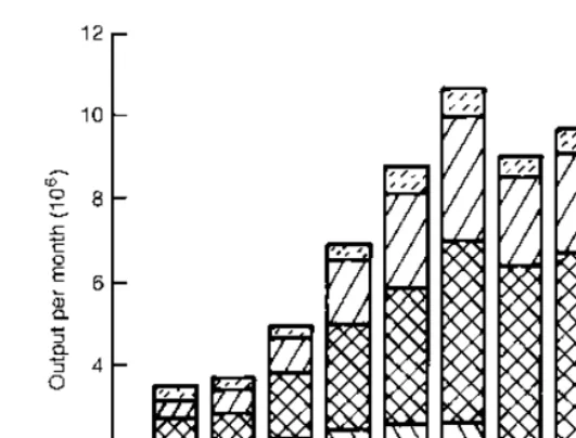
[image:41.595.100.366.68.270.2]

Perhaps the biggest single and continuing development of the last 20 years has been the application of Surface Engineering to cutting tools. In the early 1980s it was confi-dently expected that the market share for newly developed ceramic indexable insert cutting tools (for example the alumina tools considered in Section 1.4) would grow steadily, held back only by the rate of investment in the new, more powerful and stiffer machine tools needed for their potential to be realized. Instead, it is a growth in ceramic (titanium nitride, titanium carbide and alumina) coated cutting tools that has occurred. Figure 1.29 shows this. It is always risky being too specific about what will happen in the future.

(42)

References

Ashby, M. F. (1992) Materials Selection in Mechanical Design. Oxford: Pergamon Press.

Boothroyd, G. and Knight, W. A. (1989)Fundamentals of Machining and Machine Tools, 2nd edn. New York: Dekker.

(43)

2

Chip formation fundamentals

Chapter 1 focused on the manufacturing organization and machine tools that surround the machining process. This chapter introduces the mechanical, thermal and tribological (fric-tion, lubrication and wear) analyses on which understanding the process is based.

2.1 Historical introduction

Over 100 years ago, Tresca (1878) published a visio-plasticity picture of a metal cutting process (Figure 2.1(a)). He gave an opinion that for the construction of the best form of tools and for determining the most suitable depth of cut (we would now say undeformed chip thickness), the minute examination of the cuttings is of the greatest importance. He was aware that fine cuts caused more plastic deformation than heavier cuts and said this was a driving force for the development of more powerful, stiffer machine tools, able to make heavier cuts. At the same meeting, it was recorded that there now appeared to be a mechanical analysis that might soon be used – like chemical analysis – systematically to assess the quality of formed metals (in the context of machining, this was premature!).

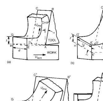
[image:43.595.77.404.484.606.2]

Three years later, Lord Rayleigh presented to the Royal Society of London a paper by Mallock (Mallock, 1881–82). It recorded the appearance of etched sections of ferrous and non-ferrous chips observed through a microscope