Full Terms & Conditions of access and use can be found at
http://www.tandfonline.com/action/journalInformation?journalCode=ubes20
Download by: [Universitas Maritim Raja Ali Haji] Date: 12 January 2016, At: 23:56
Journal of Business & Economic Statistics
ISSN: 0735-0015 (Print) 1537-2707 (Online) Journal homepage: http://www.tandfonline.com/loi/ubes20
The Decline in U.S. Output Volatility
Ana María Herrera & Elena Pesavento
To cite this article: Ana María Herrera & Elena Pesavento (2005) The Decline in
U.S. Output Volatility, Journal of Business & Economic Statistics, 23:4, 462-472, DOI: 10.1198/073500104000000596
To link to this article: http://dx.doi.org/10.1198/073500104000000596
Published online: 01 Jan 2012.
Submit your article to this journal
Article views: 57
View related articles
The Decline in U.S. Output Volatility: Structural
Changes and Inventory Investment
Ana María H
ERRERADepartment of Economics, Michigan State University, East Lansing, MI 48824 (herrer20@msu.edu)
Elena PESAVENTO
Department of Economics, Emory University, Atlanta, GA 30322 (epesave@emory.edu)
Explanations for the decline in U.S. output volatility since the mid-1980s include: “better policy,” “good luck,” and technological change. Our multiple-break estimates suggest that reductions in volatility since the mid-1980s extend not only to manufacturing inventories, but also to sales. This finding, along with a concentration of the reduction in the volatility of inventories in materials and supplies and the lack of a significant break in the inventory–sales covariance, imply that new inventory technology cannot account for most of the decline in output volatility.
KEY WORDS: Gross domestic product variance; Structural break.
1. INTRODUCTION
In recent years, several authors have documented a decline in U.S. output volatility since the mid-1980s. Using differ-ent econometric methods, both Kim and Nelson (1999) and McConnell and Perez-Quiros (2000) found evidence of a struc-tural break in volatility at the beginning of 1984. Various studies have indicated that the reduction in volatility is not con-fined to aggregate output, but extends to other aggregate vari-ables, such as all of the major components of gross domestic product (GDP) (McConnell, Mosser, and Perez-Quiros 1999), aggregate unemployment (Warnock and Warnock 2000), ag-gregate consumption and income (Chauvet and Potter 2001), and wages and prices (Sensier and Van Djik 2001; Stock and Watson 2002). Only interest rates, exchange rates, stock prices, money, and credit series have experienced upward shifts in volatility (Sensier and Van Djik 2001; Stock and Watson 2002). These findings have bolstered a line of research that seeks to understand the causes of this shift in economic behavior. Three competing explanations are better policy, better technology, and good luck. The proponents of the first hypothesis (Clarida, Gali, and Gertler 2000; Boivin and Giannoni 2003) claim that a sig-nificant change in the monetary policy rule during the Volcker– Greenspan period was the main source of this break. A second explanation advanced by McConnell and Perez-Quiros (2000) and Kahn, McConnell, and Perez-Quiros (2002) argues that the introduction of better inventory management technology is the key to understanding the break in the variability of production. Central to this hypothesis is the finding of a reducted ratio of inventory to sales volatility, which coincides roughly with the introduction of just-in-time inventory techniques, and the lack of a break in the variance of sales. Finally, Ahmed, Levin, and Wilson (2002) have contended that the decline in volatility is just a result of “good luck”—that is, a reduction in the shocks hitting the economy during the last two decades. They identified the contribution of “good luck” or smaller shocks with the high-frequency component of the GDP spectrum, low high-frequency with technological change, and the medium range of the frequency domain with monetary policy. They concluded that most of the reduction in volatility was caused by a decrease in the size of the innovations, a behavior that could be consistent with both
“good luck” and “better policy” in the form of improved mone-tary policy that worked to reduce aggregate volatility.
We extend the previous work by studying inventories and sales at a more disaggregate level, using the test of Bai and Perron (1998) for multiple breaks instead of tests for single breaks. The motivation for the higher level of disaggregation is twofold. On one hand, cross-sectional aggregation can intro-duce changes in the time series properties of the data, possibly affecting the location of the break. Furthermore, a framework that does not treat input (i.e., materials and work in process) and output (i.e., finished goods) inventories separately makes it impossible to distinguish among factors that affect the volatil-ity of these variables in a different manner. Recent work by Humphreys, Maccini, and Schuh (2001) has suggested that the response of inventories to demand shocks differs across durable and nondurable industries, as well as by stages of produc-tion. The stylized facts that these authors presented indicate that input inventories are twice as large and three times more volatile as output inventories and are particularly important in the durable goods industries. According to their estimates, the response of output inventories to demand shocks would lag the response of input inventories, and it would be smaller in mag-nitude. Thus, in the pre-Volcker era, a combination of large shocks and a monetary policy rule that allowed for increases in anticipated inflation could have led to high variability in infla-tion, sales, and inventories at all stages of producinfla-tion, possibly with a smaller increase in volatility for finished goods invento-ries.
On the other hand, the 1980s transformations in the man-ufacturing sector, such as reduction in production cycles and delivery times, could have acted to lower work-in-process and finished-goods inventory levels (Milgrom and Roberts 1990). As for the volatility of inventories, one could conjecture that given a fixed variability in the sales process, the introduction of new technologies could have resulted in faster and smaller adjustments in finished-goods and work-in-process inventories, with little change in materials.
© 2005 American Statistical Association Journal of Business & Economic Statistics October 2005, Vol. 23, No. 4 DOI 10.1198/073500104000000596
462
Our results show that the decline in the variance is a phe-nomenon that extends not only to manufacturing inventories, but also to sales. Furthermore, we show that materials and sup-plies, not finished goods, account for most of the reduction in the variance of total inventories in the 1980s. Our findings of (a) a break in sales, (b) no significant change in the inventory– sales covariance, and (c) a break in inventories that is accounted for mainly by materials and supplies lead us to conclude that the introduction of new inventory-holding techniques is insuffi-cient to explain the reduction in output volatility. These results suggest that future research on the behavior of output volatility should seek to explain not only the decline in the variance in the mid-1980s, but also the heightened volatility of the 1970s. Moreover, any theory linking better technology (in the form of better inventory management and production techniques) and reduced output volatility should focus on the role of input in-ventories.
The remainder of this article is organized as follows. Sec-tion 2 describes the industry-level data. SecSec-tion 3 reviews the test and estimation techniques for breaks of unknown timing and presents the structural break estimates. Section 4 discusses time-aggregation issues and presents the results for monthly data. Section 5 provides concluding remarks.
2. THE DATA
The industry-level data used in this article are manufacturing and trade sales and total inventories series from the Bureau of Economic Analysis (BEA). Specifically, we study manufactur-ing and trade sales, as well as inventories, and we disaggregate the latter by stages of production. The series are seasonally ad-justed and measured in chained dollars of 1996, spanning Jan-uary 1959 to March 2000. They comprise 19 two-digit SIC sectors, two three-digit SIC sectors (motor vehicles and other transportation equipment), and three aggregates (total manufac-turing, durable manufacturing and nondurable manufacturing).
Because we are interested in calculating the contribution of movements in sales and inventories to the variability of out-put, we transform the inventories and sales data in the following manner. Consider the standard inventory identity
Yi,t=Si,t+FHi,t, (1)
whereYi,t denotes output of sector iin period t, Si,t denotes
sales of sectori in periodt, andFHi,t denotes the final goods
inventories of sectoriat the end of periodt. The rate of output growth can be written as
•
and the variance in the rate of growth of output is given by
vary•i,t=vars•i,t+var
Typically the inventory identity (1) does not include inven-tory investment in production inputs, such as materials and
supplies or work in process. However, input inventories have been historically larger and more volatile than output inven-tories (Humphreys et al. 2001), and they are included along with output inventories in the computation of GDP. To evaluate their contribution to reduction in overall inventory volatility, we maintain the definition of output as in (1), but compute a mea-sure of materials (or work-in-process) inventories relative to the production of the sector as
•
ihi,t=
2IHi,t
Yi,t−1
, (5)
where IHi,t is the level of raw materials or work-in-process
inventories in sector i at the end of period t and Yt−1 is the
production of sectoriin periodt, computed as the sum of man-ufacturing sales and the change in final goods inventories. We use the same normalization for total inventories, as well as for the wholesale and retail trade series.
Our data and computation methods differ from those of McConnell and Perez-Quiros (2000) and Kahn et al. (2002) in the following manner. First, we use the BEA data on manufac-turing and trade, whereas those authors used goods sector data from the national income and product accounts (NIPA). An ad-vantage of using the NIPA is that they contain data on sectors that hold inventories but are not included in the manufacturing and trade data (i.e., agriculture and mining). Nevertheless, the high level of aggregation of the NIPA series makes it difficult to evaluate the contribution of improved inventory management and production techniques to the decline in U.S. output volatil-ity, especially to the change in the volatility of inventories at different stages of production.
Second, the NIPA contain data on output, whereas the manu-facturing and trade data do not. We therefore use the inventory identity to compute output. Due to the use of chain-weighted data, our computation of the contribution to growth is an ap-proximation to the real contribution (Whelan 2000). This was also the case in the work of McConnell and Perez-Quiros (2000).
Finally, whereas output in the NIPA includes investment in total inventories, we include only finished-goods inventories in our calculation of output, as is commonly done in inventory studies. Yet, estimation results (not reported herein) using total inventories to compute output are essentially the same.
3. STRUCTURAL BREAKS
In cases where the date of the break is known, testing for a structural change can be easily done using a Wald test. How-ever, when the date of the shift is unknown, the problem is complicated by the fact that the break date becomes a nuisance parameter that is present only under the alternative hypothesis, not under the null of no structural break. When this is the case, the standard asymptotic optimality properties of the Wald test do not hold.
Although tests for a single break have been commonly used in applied research, modeling a shift in the variance as a one-time change has a drawback in finite samples: the low power of the test in the presence of multiple breaks (Bai 1997; Bai and Perron 2003). This might well be the case for a series with two breaks in the variance such that the volatility increases in
the second period with respect to the first period but returns to its initial value after the second break. Bai and Perron (1998, 2003) proposed several tests for multiple breaks. We use one of these procedures and sequentially test the hypothesis oflbreaks versusl+1 breaks using a supFT(l+1|l)statistics, where the
supremum is taken over all possible partitions of the data for the number of breaks tested.
Letxi,t denote the sales
•
,si,t,and inventory,
•
hi,t,variables
defined in (4) and (5). Following Stock and Watson (2002), we test for structural breaks in the parameters of the autoregressive (AR) model,
kis the date of the break in the conditional mean, andτ is the date of the break in the conditional variance. The number of lags in the AR model is selected using the Bayes information crite-rion, with a maximum of four quarters. The number selected is usually two or three for total inventories series and one or two for sales. This formulation allows for the conditional mean and variance to possibly experience breaks at different dates. We test for parameter constancy in the conditional mean of the absolute value of the residuals in (6),
|εi,t| =α1,i+Ditα2,i+νit. (7)
Because when we test for a change in the covariance between inventories and sales we are interested in sign changes, we use εih,tεis,tas an estimate of the conditional covariance, whereεih,tis the residual for inventories andεis,t is the residual for sales from (6).
If the null of no break is rejected at a 10% significance level, we then proceed to estimate the break date using least squares (LS), divide the sample into two subsamples according to the estimated break date, and perform a test of parameter constancy for both subsamples. We repeat this process by increasing l
sequentially until we fail to reject the hypothesis of no addi-tional structural change. We refine the estimated break dates by repartition, as was suggested by Bai (1997) and Bai and Perron (1998). To impose the minimum structure on the data, we allow for different distribution of both the regressors and the error terms in the different subsamples, as well as for heterogeneity and serial correlation in the residuals.
There are a few cases in which the sequential procedure breaks down. For example, if two breaks of equal magnitude but opposite sign were present, then the procedure would stop at the first step and would point wrongly in the direction of no breaks. We carefully made sure that a failure to find any break was not due to breaks of the opposite sign. When this was the case, and all the tests indicated the presence two breaks, we side-stepped the first step of the sequential procedure and pro-ceeded with the estimation of two breaks.
Given the asymptotic distribution of the break dates (see Bai and Perron 1998), we calculate the corresponding 90% confi-dence intervals imposing a minimum structure on the regressors and the error terms in the different regimes. Because we allow
for different variances in the error in (6), the reported confi-dence intervals are asymmetric, showing greater uncertainty in the regime in which the variance is larger.
3.1 Total Inventories and Sales
Table 1 reports break estimates with the corresponding confi-dence intervals for the volatility of manufacturing sales and to-tal inventories by sectors. Table 2 gives results for higher levels of aggregation, such as durables and nondurables, for manufac-turing, wholesale, and retail trade. For all of the series where tests indicate that the null of no break can be rejected at a 10% significance level, we estimate the date of the breaks using the sequential procedure described in the previous section. Given the lack of precision of the tests and the size distortions at the end of the sample, we test for breaks only in the central 70% fraction of the data.
There are only a few industries for which we estimate two breaks, and none with more than two break points. We estimate a structural change in the mid-1980s for half of the two-digit series and all of the manufacturing aggregates. For all other in-dustries, the break dates are located in the late 1970s or in the early 1990s. Estimated breaks in the 1970s correspond to an increase in the volatility, whereas those in the 1980s represent a pronounced drop in the variance, often by as much as 50%. In all of the cases where more than one break is identified, the
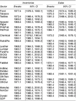
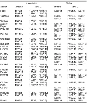
Table 1. Estimates and Confidence Intervals (CIs) for a Multiple-Breaks Date in the Conditional Variance for Total
Inventories and Manufacturing Sales
Inventories Sales
Sector Breaks 90% CI Breaks 90% CI
Food 1977:4 [1976:3, 1983:1] 1976:2 [1974:4, 1985:2] Tobacco 1975:3 [1971:1, 1976:4] Textiles 1972:4 [1966:4, 1976:3] 1991:3 [1988:4, 2002:1]
1989:2 [1988:2, 1992:2]
Apparel 1966:4 [1955:3, 1969:4] 1982:2 [1980:4, 1993:1] Paper 1983:2 [1979:3, 1995:1] Pri&Pub 1969:4 [1965:4, 1978:4] 1978:4 [1976:1, 1989:1] PetProd 1974:3 [1969:3, 1975:1] 1984:1 [1983:1, 1993:2]
1987:1 [1985:3, 1992:2]
Chemical 1981:4 [1976:2, 1983:4] 1973:2 [1965:4, 1976:1] 1990:1 [1989:1, 1994:1]
Rub&Pla 1984:4 [1983:2, 1995:2] 1967:3 [1962:3, 1969:2] 1983:4 [1982:4, 1986:3] Leather 1968:2 [1964:3, 1968:3] 1970:3 [1961:2, 1974:4] Lumber 1983:1 [1981:1, 1991:2] 1991:2 [1990:2, 1999:4] Fur&Fix 1994:2 [1991:3, 2006:3] 1983:4 [1982:1, 1990:2] StClGl 1981:4 [1980:1, 2002:2] 1993:1 [1989:2, 1997:2] PriMet 1974:2 [1971:1, 1974:4] 1984:1 [1983:2, 1988:1]
1987:4 [1987:2, 1990:1]
FabMet 1983:3 [1982:4, 1991:1] 1974:1 [1969:4, 1977:1] 1983:4 [1982:4, 1986:1] IndMac 1983:2 [1981:1, 1992:1] 1991:2 [1990:1, 1999:3] EleMac 1987:1 [1984:3, 1993:3]
MotVeh 1983:4 [1983:2, 1986:3] 1983:4 [1981:1, 1991:4] OthTran 1969:3 [1957:1, 1970:2]
Instru 1969:4 [1960:3, 1973:1] 1984:2 [1982:3, 1989:1] OthDur 1971:1 [1960:2, 1976:4] 1971:4 [1966:4, 1972:3] 1981:2 [1980:1, 1985:2] Manufac 1985:1 [1982:3, 2000:2] 1983:4 [1982:3, 1990:4] NonDur 1973:2 [1965:4, 1974:1] 1971:3 [1968:2, 1972:2] 1986:4 [1986:2, 1991:1] 1983:2 [1982:3, 1985:3] Durabl 1985:1 [1984:2, 1990:1] 1983:4 [1982:4, 1989:2] GDP 1983:4 [1982:3, 1988:4]
NOTE: See Appendix A for explanations of the abbreviations in the “Sector” column.
Table 2. Multiple-Break Test for Conditional Variance for Aggregates at Different Stages of Production
Inventories Sales
Aggregation Sector Breaks 90% CI Breaks 90% CI
Materials Manuf 1986:2 [1985:1, 1993:2] NonDur 1987:2 [1985:3, 1994:2] Durabl 1985:1 [1983:2, 1992:1] Work in process Manuf
NonDur 1979:3 [1974:1, 1982:3] 1987:3 [1985:3, 1989:3] Durabl
Finished goods Manuf 1972:1∗ [1965:2, 1974:3]
1985:1 [1982:3, 1992:2] NonDur 1971:4 [1964:3, 1972:3] 1982:3 [1981:2, 1991:1] Durabl
Wholesale trade Manufac 1972:3 [1965:2, 1974:1] 1973:1 [1958:4, 1975:2] 1983:3 [1982:3, 1989:2]
NonDur 1992:2 [1989:1, 2010:1] 1972:1 [1955:2, 1977:4] Durabl 1981:4 [1977:4, 2007:3] 1974:3 [1965:3, 1977:2] Retail trade Manuf 1992:1 [1990:3, 1997:3]
NonDur 1968:1 [1966:1, 1973:3] 1973:2 [1962:2, 1975:2] Durabl 1970:3 [1965:3, 1972:3] 1979:2 [1973:3, 1984:4] 1988:3 [1987:3, 1992:2] 1991:1 [1990:2, 1994:2]
NOTE: See Appendix A for explanations of the abbreviations in the “Sector” column.
∗Indicates cases in which the Sup-F(0 vs. 1) test failed to reject while the Sup-F(0 vs. 2) did not. All other tests [Umax, Dmax, and
Sup-F(2|1)] (see Bai and Perron 1998) also point in the direction of two breaks. In this case the estimated breaks come from the global optimization. (For a discussion on when the sequential procedure breaks down, see Bai and Perron 2003.)
Breaks in the conditional variance are computed taking into account breaks in the conditional mean.
volatility increased in the second period and subsequently re-verted to a lower volatility similar to that of the first period. In
fact, for most of the series where two breaks are estimated, one break is in the early 1970s and the other is in the mid-1980s.
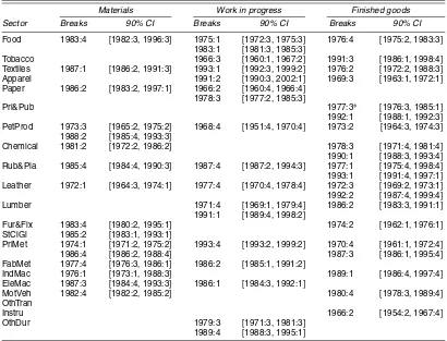
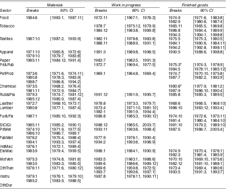
Table 3. Estimates and CIs for a Multiple-Breaks Date in the Conditional Variance for Different Stages of Production
Materials Work in progress Finished goods
Sector Breaks 90% CI Breaks 90% CI Breaks 90% CI
Food 1983:4 [1982:3, 1996:3] 1975:1 [1972:3, 1975:3] 1976:4 [1975:2, 1983:3] 1983:1 [1981:3, 1985:3]
Tobacco 1966:3 [1960:1, 1967:2] 1991:3 [1986:1, 1998:4] Textiles 1987:1 [1986:2, 1991:3] 1993:1 [1992:3, 1999:2] 1976:2 [1972:2, 1988:3] Apparel 1991:2 [1990:3, 2002:1] 1969:3 [1963:1, 1972:1] Paper 1986:2 [1983:2, 1997:1] 1966:2 [1960:4, 1966:4]
1978:3 [1977:2, 1985:3]
Pri&Pub 1977:3∗ [1976:3, 1985:1]
1992:1 [1988:1, 1992:3] PetProd 1973:3 [1965:2, 1975:2] 1968:4 [1951:4, 1970:4] 1973:2 [1964:3, 1974:3]
1988:2 [1985:4, 1993:3]
Chemical 1981:2 [1972:2, 1986:2] 1978:3 [1971:4, 1981:4] 1990:1 [1988:3, 1993:4] Rub&Pla 1985:4 [1984:4, 1990:3] 1987:4 [1987:2, 1994:3] 1977:1 [1975:4, 1998:4] 1993:1 [1991:4, 1997:1] Leather 1972:1 [1964:3, 1974:1] 1977:4 [1970:4, 1978:4] 1972:3 [1969:2, 1973:1] 1992:2 [1987:4, 1999:4] Lumber 1971:4 [1969:1, 1979:4] 1986:2 [1983:3, 1991:1]
1991:1 [1989:4, 1998:2]
Fur&Fix 1983:4 [1980:2, 1995:1] 1974:2 [1962:1, 1976:1] StClGl 1985:2 [1983:1, 1993:1]
PriMet 1974:1 [1971:2, 1975:2] 1993:4 [1993:2, 1999:2] 1970:4 [1961:1, 1972:4] 1986:4 [1986:2, 1988:4] 1987:3 [1986:1, 1995:4] FabMet 1977:4 [1976:3, 1986:1] 1986:2 [1985:1, 1991:2]
IndMac 1976:1 [1973:1, 1988:3] 1989:1 [1986:4, 1997:4] EleMac 1987:3 [1984:4, 1993:3] 1986:1 [1984:3, 1992:1]
MotVeh 1982:4 [1982:2, 1985:2] 1980:4 [1978:3, 1989:4] OthTran
Instru 1966:2 [1954:2, 1967:4]
OthDur 1979:3 [1971:3, 1981:3] 1989:4 [1988:3, 1995:1]
NOTE: See Appendix A for explanations of the abbreviations in the “Sector” column.
∗Indicates cases in which the Sup-F(0 vs. 1) test failed to reject while the Sup-F(0 vs. 2) did not. All other tests [Umax, Dmax, and Sup-F(2|1)] (see Bai
and Perron 1998) also point in the direction of two breaks. In this case the estimated breaks come from the global optimization. (For a discussion on when the sequential procedure breaks down, see Bai and Perron 2003.)
Breaks in the conditional variance are computed taking into account breaks in the conditional mean.
The first-period estimated mean variance of nondurable inven-tories is .0027; after the second quarter of 1973, it almost dou-bles to .0044, and then in 1987 it falls again to a value of .0021. This result agrees with the findings of Blanchard and Simon (2001), who contended that the observed decline in volatility was due not to a one-time break in the 1980s, but rather to a return to the lower volatility of the 1960s.
For most of the series, the break date is estimated with a low degree of precision; that is, the confidence intervals cover a large number of years. Nevertheless, in a few sales series (i.e., rubber and plastics, fabricated metals products, other durables, and nondurable manufactures) and a few inventories series (i.e., textiles, leather, primary metals products, and motor vehicles), the multiple-breaks procedure enables us to obtain estimates that are more precise with corresponding confidence intervals that span 3–5 years.
Our finding of a structural change in sales differs from the results of McConnell and Perez-Quiros (2000), but agrees with those of Ahmed et al. (2002). Differences in the date break es-timates stem from two sources. First, whereas our data span the period between the first quarter of 1959 and the first quar-ter of 2001, other researchers have analyzed data beginning in 1967. Differences in the sample period can be of significant importance in identifying the break date, because tests and esti-mates of an unknown shift point are particularly sensitive to the sample period. Because both tests and estimators are a function of the break parameterk, a possible break date that was ignored in the smaller sample can be taken into consideration when the sample is extended. Figure A.1 in Appendix A illustrates how this is the case for the variance of finished goods inven-tories of nondurable goods. The date that minimizes the sum-of-squares residuals for the 1959–2000 sample is located in the mid-1980s; yet if this test had been conducted at the beginning of the 1990s, the late 1980s data would have been eliminated by the trimming, and the break would have been estimated in the early 1970s.
A second source of divergence is related to the use of dif-ferent estimation methodologies. McConnell and Perez-Quiros (2000) estimated the break as the date associated with the max-imum of the Wald test for a single break. Instead of this ap-proach, we follow the Bai and Perron (1998) sequential testing method for multiple breaks and estimate the break date using their proposed LS estimator. Both estimates of a single break are equivalent only when the estimated relationship is linear and the residuals are homoscedastic (see Hansen 2001). In ad-dition, Bai and Perron (1998) showed that in the presence of multiple breaks, the LS estimator will converge to a global min-imum coinciding with the dominating break. A good illustration of these two sources of divergence is provided by Figure A.1, where from two possible shift points, the LS estimator selects the more pronounced one.
3.2 Inventory–Sales Covariance
Our findings of a break in the variance of manufacturing sales casts some doubts on the “technological change” hy-pothesis proposed by McConnell and Perez-Quiros (2000) and Kahn et al. (2002), who argued that the decline in the volatil-ity of GDP coincides with the development of new informa-tion technology and its applicainforma-tion to inventory management
in the durables sector. They presented two key pieces of ev-idence in support of the “better inventory management tech-niques” proposition: the differential decrease in the volatility of durables sales and production and the sign change in the co-variance between inventories and sales. These two observations are consistent with the traditional version of the production-smoothing model, where inventories act as a buffer stock to unexpected changes in sales. Yet we find that at the two-digit industry level, not only the variance of inventories but also sales has decreased, thus blurring the evidence regarding the differ-ential decrease in the volatility of sales and production. There-fore, the remaining question is whether a change in the sign of the inventory–sale covariance can account for the decline in output volatility. The answer that we derive from our results is “no.”
Results reported in Tables 4 and 5 suggest that there was a break in the conditional inventory–sales covariance in only a few two-digit manufacturing industries. This shift stemmed from changes in the generating process for sales and inventories that took place in the 1970s and 1980s. Results not reported in this article but available from the authors by request show that sectors for which the inventory volatility increased in the 1970s also experienced a simultaneous rise in the covariance, and in-dustries where inventory volatility fell in the 1980s experienced a decrease in the covariance. It is worth noting that, although the break in the covariance coincides with a decrease in inventory volatility, in almost all sectors it reflects a reduction in its mag-nitude, but not a sign change. The only exceptions to this are the covariance between finished-goods inventories and sales of
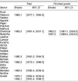
Table 4. Estimates and CIs for a Multiple-Breaks Date in the Conditional Covariance for Total Inventories and Finished
Goods Inventories With Manufacturing Sales
Total Finished goods Sector Breaks 90% CI Breaks 90% CI
Food
Chemical 1983:2 [1981:4, 2001:1] 1983:2 [1981:1, 2006:3] Rub&Pla 1987:2 [1986:4, 2003:4]
NOTE: The covariance is computed as the products of the residuals from (9) for inventories and manufacturing sales after accounting for possible breaks in the conditional means. The regressions are estimated with the same number of lags, which is chosen by the Bayes infor-mation criterion for the regression for total inventories. See Appendix A for explanations of the abbreviations in the “Sector” column.
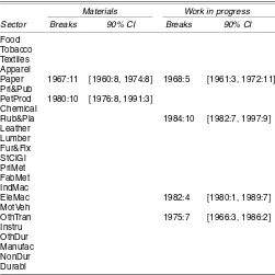
Table 5. Estimates and CIs for a Multiple-Breaks Date in the Conditional Covariance for Materials Inventories and Work-in-Progress
Inventories With Manufacturing Sales
Materials Work in progress Sector Breaks 90% CI Breaks 90% CI
Food 1972:2 [1966:1, 1978:1]
NOTE: See Appendix A for explanations of the abbreviations in the “Sector” column.
lumber and between work-in-process inventories and sales of textiles. In other words, at a two-digit industry level, we find no significant evidence that a change in the covariance, and thus in the correlation, between inventories and sales contributed to stabilize output. Our results contradict the findings of Golob (2000), who, using tests for equality of the unconditional corre-lation across the pre-1983:4 and post-1983:4 subsamples, found that inventory investment for trade and one-digit manufacturing industries has become negatively correlated with sales.
Summarizing, we estimate a decline in the volatility of in-ventories in the mid-1980s for only half of the series, and find significant evidence of a break in the variance of manufacturing sales. In addition, we find little evidence of a change in the sign of the covariance between inventories and sales. These results cast some doubts on the hypothesis that attributes the decline in output volatility to the introduction of better inventory-holding techniques and suggest that other factors must have also played an important role.
Because aggregating inventories across different stages of production might underscore the role of technology in explain-ing the reduction in the volatility of inventories and output, we examine input and output inventories separately in the next sec-tion.
3.3 Input and Output Inventories
There seems to be ample anecdotal evidence regarding the transformation that manufacturing underwent in the late twen-tieth century (Milgrom and Roberts 1990; Mosser, McConnell, and Perez-Quiros 1999). Flexible machine tools and computer-ized multitask equipment replaced specialcomputer-ized single-task
ma-chinery, allowing firms to produce a variety of output in small batches. As a result, production cycles shortened, and inven-tory holdings of work in process and finished goods dropped. Shorter production cycles led to faster order processing, re-duced product-development times, and speedier production of goods. Consequently, firms were able to increase the pace of their response to fluctuating demand and to reduce the size of back orders. Theoretical work by Milgrom and Roberts (1990) suggested that adoption of the new technologies should have resulted in “more frequent setup and smaller batch sizes, with correspondingly lower levels of finished-goods and work-in-process inventories and back orders per unit of demand.” Kahn et al. (2002), among others, provided empirical evidence of a decline in the real manufacturing inventory–sales ratios since the mid-1980s, which followed a buildup in the 1970s. How-ever, little is said in the literature about the implications of adopting the new technology for the second moment of inven-tories at different stages of production. Kahn et al. (2002), for example, presented a model in which information technology can account for a reduction in the volatility of total inventories and output, but not in that of sales. Although developing a the-oretical model that can account for the effect of technological innovation on inventory volatility is beyond the scope of this ar-ticle, we make an effort to decompose the change in inventory volatility by stages of production.
Recall that the break date estimates for total inventories (see Table 1) suggest that a reduction in volatility occurred mainly in the 1980s. These results are confirmed for the manufactur-ing aggregates (see Table 2), with the exception of invento-ries of work in process for manufacturing and durable goods and inventories of finished goods for durable manufactures. Yet at a two-digit SIC level (see Table 3), we estimate a break in finished-goods or work-in-progress inventories in the mid-1980s in only a few cases. For most industries, the shift is lo-cated in the 1970s or the 1990s; for other industries, there is no evidence of a break in work-in-progress inventories. In con-trast, we estimate a break in the 1980s for roughly half of the materials and supplies series. We derive two conclusions from the results by stages of production. First, materials and supplies account for most of the reduction in the volatility of total in-ventories during the 1980s. Furthermore, because it is only the input inventory–sales ratio that has decreased since the 1980s, if information technology played a role in reducing the volatil-ity of output, it appears to have done so by allowing firms to reduce the variation in input inventories. Second, aggregation across industries and stages of production can lead one to make a stronger statement regarding the location of the break in in-ventories in the 1980s than one would by looking at disaggre-gated data. In fact, for half of the two-digit series, if there is a break, it is not located in the 1980s. This widespread reduction in volatility across stages of production and years suggests a reduced role of information technology in explaining the mod-eration of output volatility of the 1980s.
3.4 Identifying the Break Date and the Source of the Break
One element that makes it particularly difficult to identify the source of the shift is the low degree of certainty with which
one can date the structural break. The 90% confidence inter-vals around the break can be so wide as to encompass as many as 20 years. This seems to be the case not only for invento-ries and sales, but also for a variety of macroeconomic seinvento-ries. In recent work, Stock and Watson (2002) rejected the hypoth-esis of a constant residual variance in 80% of 166 macroeco-nomic series. In most of the cases, they estimated a break in the mid-1980s; however, they also found that the 90% confidence intervals suggested break estimates that were imprecise. They argued that these confidence intervals are not very informative in the case of date break estimates that have a highly nonnor-mal distribution; thus they reported tighter 65% confidence in-tervals.
Even though in our analysis there are several cases where the 90% confidence intervals are wide, there are series for which the interval spans only 3 years, allowing us to identify the date of the break with increased precision. Hence we report 90% confidence intervals instead of the 65% ones reported by Stock and Watson (2002). Given the large degree of uncertainty re-flected in the wide confidence intervals, we believe that the es-timates of the break dates should be regarded with caution, even more so when trying to identify changes in technology, policy, or shocks that coincided with the time of the reducted output volatility.
4. EFFECTS OF TIME AGGREGATION
To make our results comparable with those of previous work, we transformed the monthly data into quarterly data by ag-gregating monthly sales and using end-of-quarter inventories. However, time aggregation may modify the time series proper-ties of the data as the magnitude of the variance decreases. Thus we replicate our estimations using the original monthly data.
Tables 6–10 report the structural break estimates and the cor-responding confidence intervals for the monthly series. Com-paring these results with those for the quarterly data suggests only a few differences. First, no break is estimated during the 1980s for manufacturing, nondurable, and durable finished goods inventories (see Table 7). However, estimates at the in-dustry level suggest a higher number of breaks in that decade than the quarterly estimates (see Table 9). Although these dif-ferences at first sight appear to be larger, careful inspection of Tables 3 and 8 reveals that there are the same number of indus-tries for which the confidence intervals cover the mid-1980s at both frequencies.
Second, although the maximum number of breaks that we estimate with the quarterly data is two, using monthly data, we estimate three breaks for total inventories of motor vehicles and inventories of materials for petroleum products. Further-more, there are a few series for which the number of estimated
Table 6. Estimates and CIs for a Multiple-Breaks Date in the Conditional Variance for Total Inventories and Manufacturing Sales, Monthly Data
Inventories Sales
Sector Breaks 90% CI Breaks 90% CI
Food 1978:3 [1976:10, 1984:7] 1982:12 [1981:4, 1987:8] 1992:5 [1990:11, 1996:4]
Tobacco 1980:11 [1975:5, 1982:3] 1978:5 [1976:5, 1978:7] 1994:2 [1993:4, 1997:1] Textiles 1989:5 [1989:1, 1992:7]
Apparel 1977:5 [1974:6, 1983:8] 1985:10 [1982:12, 1994:7]
Paper 1981:2 [1975:4, 1992:8]
Pri&Pub 1965:12 [1964:2, 1971:9] 1978:10 [1975:11, 1987:3] 1993:12 [1991:4, 2000:2] PetProd 1971:10 [1962:4, 1974:8] 1971:11 [1968:10, 1972:4] 1981:2 [1980:6, 1984:2] Chemical 1980:9 [1978:2, 1981:2] 1979:2 [1975:6, 1981:1]
1986:9 [1985:3, 1991:5]
Rub&Pla 1987:10 [1987:6, 1990:8] 1991:4 [1990:9, 1994:10] Leather 1968:7 [1965:10, 1968:12] 1970:6 [1961:8, 1974:1] Lumber 1975:4 [1973:10, 1980:12] 1989:8 [1988:10, 1994:1]
1993:9 [1991:4, 1998:1]
Fur&Fix 1993:3 [1992:10, 1995:8] 1980:9 [1976:5, 1987:10] StClGl 1987:3 [1986:5, 1993:12] 1966:2 [1962:10, 1972:11] PriMet 1987:4 [1987:1, 1994:8] 1965:9 [1964:12, 1982:12] 1992:1 [1991:10, 1996:1] FabMet 1975:6 [1972:2, 1982:8] 1982:10 [1981:11, 1986:7]
1992:3 [1991:1, 1997:10]
IndMac 1987:10 [1986:2, 1993:5] 1987:9 [1984:7, 1994:10] EleMac 1985:12 [1984:7, 1993:9]
MotVeh 1970:10 [1970:4, 1977:3] 1971:8 [1968:8, 1987:10] 1981:1 [1980:8, 1983:10] 1991:12 [1991:4, 1998:7] 1993:8 [1992:11, 1997:3]
OthTran 1993:7 [1987:10, 1998:3] 1993:6 [1998:12, 1995:8] Instru 1969:4 [1962:12, 1970:2]
OthDur 1973:8 [1970:3, 1974:5] 1985:1 [1983:9, 1988:7] Manufac 1985:2 [1983:2, 1993:10] 1980:11 [1978:10, 1989:10] NonDur 1986:12 [1982:7, 1998:1] 1972:5 [1967:5, 1975:8]
1983:6 [1982:3, 1987:3] Durabl 1984:4 [1983:6, 1990:6] 1980:10 [1979:1, 1989:1]
NOTE: See Appendix A for explanations of the abbreviations in the “Sector” column.
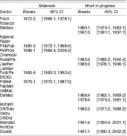
Table 7. Multiple-Breaks Test for Conditional Variance for Aggregates at Different Stages of Production, Monthly Data
Inventories Sales
Aggregation Sector Breaks 90% CI Breaks 90% CI
Materials Manuf 1986:1 [1985:8, 1989:9] NonDur 1987:1 [1986:2, 1992:2] Durabl 1983:8 [1983:4, 1988:6] Work in process Manuf
NonDur 1979:8∗ [1975:6, 1980:9] 1987:9 [1986:9, 1991:9] Durabl 1991:11 [1989:1, 2003:8] Finished goods Manuf 1991:12 [1988:7, 2001:4] NonDur 1993:2 [1990:6, 1998:10]
Durabl
Wholesale trade Manufac 1971:12 [1968:2 1973:6] 1974:2 [1969:3, 1975:10] 1987:2 [1984:2, 1993:2]
NonDur 1971:9 [1968:3, 1973:2] 1972:5 [1967:11, 1974:12] 1983:6 [1982:3, 1988:2]
Durabl 1973:8 [1969:12, 1975:3] 1974:11 [1972:2, 1975:8] 1992:11 [1990:11, 1997:1] Retail trade Manuf 1973:3 [1963:3, 1974:12]
1987:10 [1987:1, 1992:10]
NonDur 1980:4 [1978:5, 1984:6] 1973:6 [1968:3, 1976:9] Durabl 1974:7 [1966:6, 1975:5] 1993:9 [1992:4, 2008:8]
1987:10 [1987:4, 1994:4]
NOTE: See Appendix A for explanations of the abbreviations in the “Sector” column.
∗Indicates cases in which the Sup-F(0 vs. 1) test failed to reject while the Sup-F(0 vs. 2) did not. All other tests [Umax, Dmax, and Sup-F(2|1)] (see Bai and Perron 1998)
also point in the direction of two breaks. In this case the estimated breaks come from the global optimization. (For a discussion on when the sequential procedure breaks down, see Bai and Perron 2003.) Breaks in the conditional variance are computed taking into account breaks in the conditional mean.
Table 8. Estimates and CIs for a Multiple-Breaks Date in the Conditional Variance for Different Stages of Production, Monthly Data
Materials Work in progress Finished goods
Sector Breaks 90% CI Breaks 90% CI Breaks 90% CI
Food 1984:6 [1983:1, 1987:11] 1972:11 [1967:1, 1976:3] 1974:9 [1971:6, 1983:8] 1982:9 [1980:6, 1987:4] Tobacco 1978:7 [1975:12, 1979:9] 1965:11 [1965:5, 1969:8] 1984:12 [1983:8, 1989:8] 1986:8 [1984:4, 1989:9] 1994:3 [1994:1, 1998:8] Textiles 1987:10 [1987:2, 1993:9] 1982:11 [1978:8, 1983:8] 1975:5 [1975:3, 1980:5] 1988:11 [1988:9, 1991:1] 1984:1 [1980:6, 1984:11]
1994:2 [1992:8, 1998:11] Apparel 1971:10 [1965:8, 1972:6] 1991:3 [1989:8, 1996:5] 1990:5 [1988:6, 1998:8]
1979:10 [1979:7, 1983:8]
Paper 1985:11 [1984:12, 1991:4] 1983:7 [1982:5, 1991:3]
Pri&Pub 1972:7 [1969:4, 1977:5] 1975:3∗ [1974:3, 1978:9] 1984:5 [1978:11, 1985:12] PetProd 1973:6 [1971:6, 1974:11] 1969:1 [1964:8, 1969:4] 1974:7 [1970:10, 1975:8]
1980:8 [1978:3, 1983:9] 1987:7 [1982:2, 1992:9] 1988:7 [1986:8, 1994:2]
Chemical 1973:5 [1968:2, 1976:4] 1980:6∗ [1977:9, 1981:2]
1981:11 [1972:9, 1984:7] 1987:9 [1986:10, 1990:4] Rub&Pla 1979:3 [1974:7, 1981:12] 1991:12 [1991:9, 1995:7] 1985:8 [1985:3, 1989:5]
1985:12 [1985:9, 1987:4]
Leather 1972:7 [1968:10, 1973:1] 1978:8 [1973:3, 1979:7] 1968:6 [1966:5, 1968:10] Lumber 1980:8 [1977:1, 1987:4] 1973:4 [1971:10, 1981:10] 1986:10 [1983:12, 1992:4]
1992:1 [1991:9, 1994:4]
Fur&Fix 1987:1 [1985:10, 1992:3] 1986:8 [1985:3, 1990:12] 1974:10 [1972:6, 1975:11] 1981:4 [1980:4, 1984:10] StClGl 1985:11 [1985:2, 1990:1] 1988:12 [1985:5, 2003:7] 1981:10 [1979:2, 1989:10] PriMet 1974:10 [1971:9, 1977:5] 1993:11 [1993:6, 1998:4] 1987:5 [1986:7, 2005:4]
1986:10 [1986:7, 1989:1
FabMet 1976:2 [1975:4, 1988:4] 1977:9 [1976:1, 1990:4] 1994:1 [1993:3, 1997:4] 1994:2 [1993:6, 1996:9] IndMac 1976:1 [1972:1, 1989:4]
EleMac 1983:9 [1979:4, 1999:5] 1986:1 [1984:1, 1990:9] 1974:9 [1970:4, 1976:1] 1982:3 [1981:4, 1985:9] MotVeh 1975:3 [1974:8, 1981:6] 1983:5 [1983:1, 1986:6] 1970:10 [1969:10, 1975:6] 1983:5 [1983:3, 1985:5] 1989:6 [1986:6, 1989:12] 1982:12 [1981:10, 1988:1] OthTran 1976:11 [1971:6, 1980:12] 1969:6 [1959:8, 1972:5] 1973:4 [1969:4, 1980:6] 1993:7 [1990:6, 1997:1] 1993:5 [1991:3, 1993:7] Instru 1979:1 [1976:1, 1979:10] 1987:8 [1978:11, 1990:11]
1985:2 [1983:9, 1988:5] OthDur
NOTE: See Appendix A for explanations of the abbreviations in the “Sector” column.
∗Indicates cases in which the Sup-F(0 vs. 1) test failed to reject while the Sup-F(0 vs. 2) did not. All other tests [Umax, Dmax, and Sup-F(2|1)] (see Bai and Perron 1998)
also point in the direction of two breaks. In this case the estimated breaks come from the global optimization. (For a discussion on when the sequential procedure breaks down, see Bai and Perron 2003.) Breaks in the conditional variance are computed taking into account breaks in the conditional mean.
Table 9. Estimates and CIs for a Multiple-Breaks Date in the Conditional Covariance for Total Inventories and Finished Goods
Inventories With Manufacturing Sales, Monthly Data
Total Finished goods Sector Breaks 90% CI Breaks 90% CI
Food
Tobacco 1990:7 [1981:5, 1990:11] 1990:7 [1990:6, 1990:7] Textiles
NOTE: The covariance is computed as the products of the residuals from (9) for inventories and manufacturing sales after accounting for possible breaks in the conditional means. The regressions are estimated with the same number of lags, which is chosen by the Bayes infor-mation criterion for the regression for total inventories. See Appendix A for explanations of the abbreviations in the “Sector” column.
breaks increases from one to two. We believe that this result is due to the heightened variance that results from using higher-frequency data.
Table 10. Estimates and CIs for a Multiple-Breaks Date in the Conditional Covariance for Materials Inventories and Work-in-Progress
Inventories With Manufacturing Sales, Monthly Data
Materials Work in progress Sector Breaks 90% CI Breaks 90% CI
Food Tobacco Textiles Apparel
Paper 1967:11 [1960:8, 1974:8] 1968:5 [1961:3, 1972:11] Pri&Pub
NOTE: See Appendix A for explanations of the abbreviations in the “Sector” column.
Our main findings remain unchanged. We find evidence of (a) a decrease in the variance of both manufacturing inventories and sales during the 1980s, (b) a decrease in the variance of total inventories during the 1980s, (c) no structural break in the inventory–sales covariance (see Table 10), and (d) diminished volatility in inventories by stages of production, particularly in materials and, to a lesser degree, in work in process and finished goods.
Are higher-frequency data more appropriate for estimating and identifying the source of the structural breaks? The answer to this question is not clear. On one hand, it allows us to identify some additional breaks that might have been smoothed out by the time aggregation. On the other hand, the degree of precision of the estimates does not improve significantly; the confidence intervals continue to be large for various series.
5. FINAL REMARKS
We have analyzed an event that has been documented and studied in recent macroeconomic literature: the decline in U.S. output volatility. Although we confirm the finding of Mc-Connell and Perez-Quiros (2000) of a decline in the volatility of manufacturing and durable goods inventories in the 1980s, we find evidence of multiple breaks, which suggests that the structural change in the variance might not be a one-time phe-nomena. There are a number of inventory and sales series for which the decline in the variance seems to be a return to a less volatile state experienced before the volatile 1970s.
In agreement with Ahmed et al. (2002), we find that the decline in variance is a phenomenon that extends not only to manufacturing inventory series, but also to sales. In addition, we find that the decline in volatility of manufacturing invento-ries is accounted for mainly by a decline in that of materials and supplies. These findings suggest that the introduction of better inventory tracking technology only partly explains the decline in output volatility. We agree with Stock and Watson’s (2002) conclusion that better monetary policy may account for some of the moderation in the volatility of output. We can expect at least some of the lower volatility to continue if the monetary rule is maintained.
Thus two relevant features of our results are that (a) inven-tories of materials and supplies played an important role in ac-counting for the decline in inventory and output volatility, and (b) breaks in the variance of inventories and sales are not a one-time phenomena. These two features of the data should be taken into account by business cycle theorists, as well as by re-searchers seeking to explain the decrease in U.S. output volatil-ity.
ACKNOWLEDGMENTS
The authors thank Bruce Hansen, Jushan Bai, and Pierre Per-ron for making their GAUSS codes available. They also thank Margaret McConnell, the associated editor, two anonymous ref-erees, seminar participants at Michigan State University, Wayne State University, Emory University, and Université de Montréal for helpful comments. Any remaining errors are the authors’.
APPENDIX A: WALD TEST FOR BREAK TESTING
Figure A.1. LS Break Date Estimation: Residual Variance as a Func-tion of Break Date.
Figure A.2. Testing for Structural Change Inventories: Nondurables Lags ( , Chow test sequence; , Andrews critical value; - - , chi-squared critical value).
Figure A.3. Testing for Structural Change Inventories: Nondurables Intercept ( , Chow test sequence; - - , Andrews critical value; , chi-squared critical value).
Figure A.4. Testing for Structural Change of Unknown Timing: Chow Test Sequence as a Function of Break Date ( , Chow test sequence; - - , Andrews critical value; , chi-squared critical value).
Figure A.5. Inventories: Nondurables Estimation of Break Date in Variance.
Figure A.6. Inventories: Nondurables Wall Sequence for Variance ( , Wald sequence; - - , asymptotic critical value).
APPENDIX B: ABBREVIATIONS IN “SECTOR” COLUMN IN TABLES 1–10
Sector Abbreviation
Food Food
Tobacco Tobacco
Textiles Textiles
Apparel Apparel
Paper Paper
Printing and publishing Pri&Pub Petroleum products PetProd Chemicals Chemical Rubber and plastics Rub&Pla
Leather Leather
Lumber Lumber
Furniture and fixtures Fur&Fix Stone, clay and glass products StClGl Primary metals products PriMet Fabricated metals products FabMet Industrial machinery IndMac Electrical machinery EleMac Motor vehicles MotVeh Other transportation equipment OthTran Instruments Instru Other durable manufactures OthDur Manufacturing Manufac Nondurables NonDur Durables Durabl
[Received June 2003. Revised June 2004.]
REFERENCES
Ahmed, S., Levin, A., and Wilson, B. A. (2002), “Recent U.S. Macroeconomic Stability: Good Luck, Good Policies, or Good Practices?” International Fi-nance Discussion Papers 2002–2730, The Board of Governors of the Federal Reserve System.
Bai, J. (1997), “Estimation of a Change Point in Multiple Regression Models Estimating and Testing Linear Models With Multiple Structural Changes,”
Review of Economics and Statistics, 79, 551–563.
Bai, J., and Perron, P. (1998), “Estimating and Testing Linear Models With Multiple Structural Changes,”Econometrica, 66, 47–78.
(2003), “Computation and Analysis of Multiple Structural Change Models,”Journal of Applied Econometrics, 18, 1–22.
Blanchard, O., and Simon, J. (2001), “The Long Decline in U.S. Output Volatil-ity,”Brookings Papers on Economic Activity, 1, 135–173.
Boivin, J., and Giannoni, M. (2003), “Has Monetary Policy Become More Ef-fective?” NBER Working Paper 9459, National Bureau of Economic Re-search.
Chauvet, M., and Potter, S. (2001), “Recent Changes in the U.S. Business Cy-cle,”Manchester School of Economic and Social Studies, 69, 481–508. Clarida, R., Gali, J., and Gertler, M. (2000), “Monetary Policy Rules and
Macroeconomic Stability: Evidence and Some Theory,”The Quarterly Jour-nal of Economics, 115, 147–180.
Golob, J. E. (2000), “Post-1984 Inventories Revitalize the Production-Smoothing Model,” unpublished working paper.
Hansen, B. E. (2001), “The New Econometrics of Structural Change: Dating Breaks in U.S. Labor Productivity,”The Journal of Economic Perspectives, 15, 117–128.
Humphreys, B. R., Maccini, L. J., and Schuh, S. (2001), “Input and Output Inventories,”Journal of Monetary Economics, 47, 347–375.
Kahn, J. A., McConnell, M. M., and Perez-Quiros, G. (2002), “On the Causes of the Increased Stability of the U.S. Economy,”Economic Policy Review, 8, 183–206.
Kim, C., and Nelson, C. R. (1999), “Has the U.S. Economy Become More Sta-ble? A Bayesian Approach Based on a Markov-Switching Model of Business Cycle,”The Review of Economics and Statistics, 81, 608–616.
McConnell, M. M., Mosser, P., and Perez-Quiros, G. (1999), “A Decomposition of the Increase Stability of GDP Growth,”Current Issues in Economics and Finance, 5, 1–6.
McConnell, M. M., and Perez-Quiros, G. (2000), “Output Fluctuations in the United States: What Has Changed Since the Early 1980’s?”American Eco-nomic Review, 90, 1464–1476.
Milgrom, P., and Roberts, J. (1990), “The Economics of Modern Manufactur-ing: Technology, Strategy, and Organization,”American Economic Review, 80, 511–528.
Mosser, P., McConnell, M. M., and Perez-Quiros, G. (1999), “A Decomposition of the Increased Stability of GDP Growth,”Current Issues in Economics and Finance, 5, 1–6.
Sensier, M., and Van Djik, D. (2001), “Short-Term Volatility versus Long-Term Growth: Evidence in U.S. Macroeconomic Time Series,” Discussion Paper 8, University of Manchester.
Stock, J. H., and Watson, M. W. (2002), “Has the Business Cycle Changed and Why?” inNBER Macroannual 2002, eds. M. Gertler and K. Rogoff, Cambridge, MA: MIT Press, pp. 159–218.
Warnock, M. V. C., and Warnock, F. E. (2000), “Explaining the Increased Vari-ability in Long-Term Interest Rates,”Economic Quarterly, 85, 71–96. Whelan, K. (2000), “A Guide to the Use of Chain-Aggregated NIPA Data,”
Finance and Economics Discussion Series, 2000–2035, The Board of Gov-ernors of the Federal Reserve System.