on Health over the Life-Course
James P. Smith
a b s t r a c t
Using data from the PSID, across the life course SES impacts future health outcomes, although the primary influence is education and not an individual’s financial resources in whatever form they are received. That conclusion appears to be robust whether the financial resources are income or wealth or whether the financial resources represent new information such as the largely unanticipated wealth that was a consequence of the recent stock market boom. Finally, this conclusion is robust across new health outcomes that take place across the short and intermediate time frames of up to 15 years in the future.
I. Introduction
It is well documented that individuals with lower socioeconomic sta-tus (SES) have much worse health outcomes (Marmot 1999; Smith 1999). But why this is so continues to be debated (Adamset al. 2003; Deaton 2003). The central question is whether these large differences in health by such SES indicators as in-come, wealth, or education largely reflect causation from SES to health or instead the cumulative consequences of poor health outcomes throughout one’s life. Even if SES mainly affects health, what dimensions of SES actually matter—financial aspects such as income or wealth or nonfinancial dimensions like education?
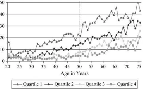
This paper begins with the perspective that there is a distinct life-course compo-nent to the health-SES gradient so that we may be misled in trying to answer these questions by only looking at people of a certain age—say those past age 50 as re-quired by the widely used Health and Retirement data (HRS). To see this, Figure 1, which is based on the PSID, displays the main contours of the SES-health gradient by plotting at each age the fraction of people who report themselves in fair or poor
James P. Smith holds the RAND chair in Labor Market and Demographic Studies. He would like to thank the helpful advice and assistance from Bob Schoeni. Programming assistance of Patty St. Clair and David Rumpel is gratefully appreciated. This paper benefited from comments by participants at seminars at Princeton University and the Population Council. This research was supported by grants from NIA. The data used in this article can be obtained beginning May 2008 through April 2011 from James P. Smith, 1776 Main Street, PO Box 2138, Santa Monica, CA 90407-2138. smith@rand.org. [Submitted August 2005; accepted November 2007]
ISSN 022-166X E-ISSN 1548-8004Ó2007 by the Board of Regents of the University of Wisconsin System
health by age-specific household income quartiles.1At least until the end of life, for the most part at each age every movement down in income is associated with being in poorer health. Moreover, the health differences by income class are quite large. The fraction in fair or poor health in the top income quartile is often 30 percentage points smaller than the fraction in those health groups in the lowest income quartile. Finally, there is a quite distinct age pattern to the SES-health gradient with health disparities by income class expanding up to around age 50, after which the health gradient begins slowly to fade away.
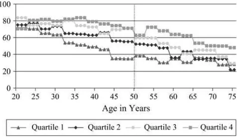
Figure 2 illustrates that a quite similar pattern emerges when our SES measure shifts to an important SES market-household wealth—an expanding health gradient into middle age followed by a gradual contraction.2Given the dramatic age patterns to the SES health gradient, the value of panels such as the PSID that span the entire life course in addressing these difficult questions about the meaning of the SES-health gradient would seem to be potentially quite high.
This paper is divided into four sections and an appendix. Section I is the introduc-tion; Section II describes health and other relevant data available in the Panel Study of Income Dynamics (PSID). In recent years, the PSID has added significant health content to its core module. The appendix to the paper provides an evaluation of the Figure 1
Percent Reporting Fair or Poor Health Status by Age-Specific Income Quartiles
To construct this figure, individuals in each age-year cell between the years 1984 and 1999 were separated into four age-specific household income quartiles, and the self-reported health status of each group was computed. The data were merged across all years.
1. The data in Figure 1 are calculations by the author from the PSID. To construct this figure, individuals in each age-year cell between the years 1984 and 1999 were separated into four age-specific household in-come quartiles and the self-reported health status of each group was computed. The data were merged across all years. For similar graphs, see Case and Deaton (2005).
quality of this new mostly retrospectively collected health data for the type of re-search conducted in this paper. Section III examines the effect of SES on health by looking at whether the onset of new chronic conditions is related to household income, wealth, and education—once one conditions of a set of preexisting demo-graphic and health conditions. This analysis attempts to take advantage of three unique features of the PSID for this type of analysis—tracking health onsets well into the future, assessing whether the predictive effects of the main SES measures vary with age, and reconstructing an individual’s prior SES and health history with its long-term panel. The final section of the paper contains the conclusions.
II. Data
The Panel Study of Income Dynamics (PSID) has gathered almost 30 years of extensive economic and demographic data on a nationally representative sample of approximately 5,000 (original) families and 35,000 individuals who live in those families. There are several potential advantages to using the PSID to study issues surrounding the SES-health gradient. In contrast to the other panel surveys such as the HRS and AHEAD that have been widely used to investigate the SES-health gradient, the PSID spans all age groups, allowing one to examine behavior over the complete life cycle. Figures 1 and 2 have already indicated that the nature of the SES-health gradient may differ significantly across age groups.
The PSID is recognized as one of the premiere general-purpose panel surveys measuring several key dimensions of SES. Details on family income and its compo-nents have been gathered in each wave since the inception of PSID in 1968. Starting in 1984 and in five-year intervals until 1999, PSID asked a set of questions to Figure 2
Percent Reporting Excellent or Very Good Health Status by Age-Specific Wealth Quartiles
measure household wealth. Starting in 1997, the PSID switched to a two-year peri-odicity, and wealth modules are now included as part of the core interview.
The PSID has been collecting information on self-reported general health status (the standard five-point scale from excellent to poor) since 1984. Starting in 1999 and for all subsequent waves, PSID has collected information on the prevalence and incidence of a list of chronic conditions—heart disease, stroke, heart attack, hy-pertension, cancer, diabetes, chronic lung disease, asthma, arthritis, and emotional, nervous, or psychiatric problems. In addition to the prevalence in 1999, individuals were asked the date of onset of the condition and whether it limited their normal daily activities. Thus keeping in mind issues related to recall bias, the implications of which I discuss in the appendix, the timing of a health onset can potentially be identified and the impact of these new health events on labor supply, income, and wealth can be estimated.3
The PSID offers several key potential additions to the research agenda. First, as Figures 1 and 2 suggest, the nature of the SES-health gradient may vary considerably over the life cycle. For example, during the age span covered by HRS, the income-health gradient was actually becoming considerably smaller. Labor supply effects in-duced by new health events may be very sensitive to life-cycle stage as for onsets that take place in the late mid-50s or earlier-60s individuals can select an option that they would have chosen in a few years anyway—retirement.
Second, the long-term nature of the PSID allows one to estimate the impact of health and SES innovations over relatively long periods—at this point measured in decades. It may well be that health responds to changes in financial measures of SES but only after a considerable lag. Third, the PSID also permits a unique long-term perspective in the other direction. Given that many panel members have been members of the PSID since 1967, the entire past sequence of financial situation can be exploited in the research. Current or last year’s income alone may be an inadequate proxy for a household’s command over financial resources either due to standard classical mea-surement error issues or the familiar distinction between current and permanent in-come (Friedman 1957). While the British cohort samples are an important research tool for studying the prospective evolution of both SES and health, no other American survey can match the long history of financial SES information now available in the PSID.
The two elements of the expanded PSID health content that potentially are ana-lytically useful are the prospectively collected general health status available yearly since 1984 and the 1999 retrospective health conditions information. In my view, there is too much noise in year-to-year changes in general health status for it to be used as an index of new health onset (Crossley and Kennedy 2002). But this past information on general health status remains useful in that it captures at least part of the past health histories of individuals, information that is necessary to separate out the predictable and unpredictable components of new health onsets. Following Smith (1999), onsets of chronic health conditions can be used to measure new health onsets.
III. Predicting the Onset of Future Health Conditions
A. Conceptual Issues
In this section, I explore the pathway from SES to health by examining whether the future onset of new chronic conditions is related to levels of household income, wealth, and education, once one conditions of a set of preexisting set of demo-graphic, economic, and health conditions. Before summarizing those results, it is useful first to outline the essential issues in estimating effects of SES on health. Fol-lowing the treatment in Smith (1999) and Adams et al. (2003), current realizations of both economic status and health reflect a dynamic history in which both health (Ht)
and SES (Yt) are mutually affected by each other as well as by other relevant forces.
Most of the relevant ideas can be summarized by the following equation:
Ht¼a0+a1Ht21+a2Yt21+a3DYˆt+a4Xt21+u1t
ð1Þ
whereXt-1 represents a vector of other possibly nonoverlapping time and nontime
varying factors influencing health and SES andu1tare stochastic shocks to health. In this framework, we can estimate whether past values of SES predict health (a26¼ 0).4In the tradition of Granger causality, one view is that this provides a test of no direct causal path (conditional onHt21) betweenYt21andHt.
5More precisely, this
reduces to a joint test that there is not a direct causal link betweenYt21andHtand no
unobserved common factors that could create an ecological correlation betweenYt21
andHt. Since it is in general impossible to rule out the possibility of all such
unob-served factors, some caution is warranted in going beyond the language of prediction with these parameters on lagged values.a2may be better viewed, as it will be here, simply as the ability of past values of SES to predict future health onsets. The reason is that there may well be unobserved factors correlated both with past SES and health, even after we have conditioned on the measured components.
But even with this caution, the estimated values ofa2may be suggestive in the cau-sality debate. Many unobserved factors would tend to produce a positive correlation be-tween past SES and health biasinga2upward. Health is a central part of human capital and is positively correlated with other components of human capital that lead one to have higher earning capacity. Even in a data source as rich as PSID, not all the compo-nents of health or other dimensions of human capital that produce higher SES can be measured adequately. Thus, some of them surely appear as a positive correlation in past SES and unobserved dimensions of health. In this case, the coefficients on past SES var-iables would be overstating the true effect of SES on health.
Of course, it is not possible to strictly sign the bias ina2since there are other fac-tors that would lead to a downward bias ina2. One obvious example would be clas-sical measurement error in past SES, which would biasa2toward zero. However, this
4. For an insightful debate about the conditions under whether coefficients are zero or stationary also reveals something about causality, see the paper by Adams et al. (2003) and the comments on that paper in the same volume.
type of bias can be mitigated by standard practices such as averaging past values of SES or including long lag structures in SES, which is what is done in this paper.
Another key parametera3measures the effect of new innovations of SES (DYˆt) on health. The termDYˆtrepresents that part of the between period change in SES (DYt) that is an innovation. To estimatea3, we require exogenous variation in SES (DYˆt) not induced by health. In particular, this implies that it is not appropriate to use the full between-period changes SES (DYt) to estimate these effects since such var-iation hopelessly confounds feedback effects. For example, a new health problem could reduce labor supply and hence income so that regressing the change in health on the change in income would have it all backward.
One opportunity for estimating the effects of SES not caused by health lies in the large wealth increases that were accumulated during the large stock market runup during the late 1980s and 1990s. Given the unusually large runup in the stock market during these decades, it is reasonable to posit that a good deal of this surge was unanticipated and thus captures unanticipated exogenous wealth increases that were not caused by a person’s health. If financial measures of SES do improve health, such increases in stock market wealth should be associated with better subsequent health outcomes at least with a lag. While this empirical approach is followed in this paper, it is certainly not without its drawbacks. One legitimate criticism in my view is that—given the distribution of stock market capital gains in the population—we essentially end up studying the av-erage treatment effect of ‘‘exogenous’’ financial wealth changes on health for mostly the very well-to-do. Not only may we be missing the policy relevant part of the pop-ulation, but the average health change induced by these innovations in the financial dimensions of SES are measured across a population whose health is very good to begin with and whose health is probably less likely to change.
Another relevant issue looks deeper at the source of the variation in stock wealth used in estimating the impact. There is a key conceptual difference between within-individual variation in stock wealth overt,on which the surge in the stock market argument relies, and point in time variation acrossi,or across individuals. Variation acrossimay not yield unbiased estimates if those who are have greater current ex-posure to stock market gains by investing more in the past in the stock market are healthier. Some of this possible contamination is dealt with by the extensive con-trols for past health that are included in the models estimated below, but there still remains the possibility of unobserved components of health that are correlated with the size of the stock market exposure people have.6While it undoubtedly helps to be estimating within a time period in which the variation acrosstis so large, one must acknowledge that the variation on which these estimates rely combine variation acrossiandt.
A third issue is that there may be good reason to distinguish between effects of pos-itive wealth gains and negative wealth losses on health onsets since they may have asymmetric effects on health. There may not be a plausible mechanism (for those al-ready with health insurance) that explains why making a good deal of extra money makes one healthier or happier, especially if one quickly adjusts to the new state. In
contrast, unexpectedly large poor financial outcomes may lead to distress, worry, and depression as one tries to make ends meet in the new financial reality. Many epidemiological studies show that prolonged periods of psychological stress may have negative consequences for one’s health (Steptoe and Marmot 2004). Fortunately, the problem of asymmetric impacts is more easily dealt with empirically since we can distinguish capital gains and capital losses in the empirical specification. I report results from several tests of this distinction between capital gains and capital losses below.
The fundamental difference between estimates of the relation between SES and health that are obtained from estimates of models like Equation 1 compared to the strong relation between health and SES that exists in Figures 1 and 2 do not simply flow from these distinctions involved in isolating new information in the measures of SES. A more critical issue in fact involves how one measures health. A good deal of the evidence that claims that there is a strong relationship between all measures of SES and health uses some stock measure of health as the outcome variable. These stud-ies are largely cross-sectional and typically use measures such as current general health status, disease prevalence rather than incidence, or mortality as the health out-come. Such stock measures of health hopelessly confound all past interactions be-tween health and SES, no matter which direction of causation bebe-tween the two was operative or how important some third factor was in influencing both health and SES. In this paper, I follow instead the suggestion first made in Smith (1999) of using the onset of new health conditions as the health outcome. The advantage of using new health onsets is that one is at least attempting to isolate new health events that are distinguishable from past health, especially when one simultaneously controls for comprehensive measures of past health status, past health behaviors, and SES. Even with a data set as rich as the PSID, one still must always acknowledge that there may be information about past health available to the individual but not to the statistical analyst. An alternative view is that this may be pushing individual rationality a bit too far if people do not fully incorporate the risks inherent in their health behaviors in formulating their views about their future health trajectories.
It is possible to estimate models based on Equation 1 with health outcomes besides new onsets as long as one still conditions on a comprehensive array of past values of health and SES as implied by Equation 1. A good case in point would be mortality. Moreover, there would be no inherent contradiction between finding no influence of financial measures of SES on disease onset but in finding an influence on subse-quent mortality. It may well turn out that economic resources have significant impacts on mortality but not on disease onset suggesting that the main influence of financial resources is not in preventing disease onset but in dealing more effec-tively with treatment of an illness after it occurs thereby mitigating its impact on sub-sequent mortality.7
B. Empirical Estimates
The key implication of Equation 1 is that one should condition on the full array of base-line health and SES status to estimate the relation between SES and health. The models I estimate include as covariates a vector of baseline health conditions of the respon-dent—self-reported general health status (excellent, very good, good, fair with poor the left-out group) and the presence of chronic conditions (arthritis, cancer, diabetes, heart disease, hypertension, lung disease, and stroke) all measured at baseline. The models include a standard set of demographic controls—age (dummies for whether one is 51–61 years old or age 62 and older), race (dummy for African-American), eth-nicity (dummy for Hispanic), sex (dummy for female), marital status and marital tran-sition between waves, employment, home ownership, and state of residence.8
The PSID only allows one to back-cast one health behavior so that one can con-dition on it at each baseline year in the analysis. Fortunately, it is the most important health behavior—smoking—well known to be highly correlated with both education and income. Three smoking-related variables are included in these models—whether one ever smoked before baseline, whether one currently smoked at baseline, and the number of cigarettes normally smoked.
The principal interest lies in evaluating the importance of various SES measures that include household income, baseline levels of and exogenous changes in house-hold wealth, and respondent’s education. SES is not a one-dimensional concept and knowing which aspect of SES affects health is key to the policy debate surrounding the SES-health gradient. If the only pathway that operates from SES to health is ed-ucation, policies directed at income redistribution could not be justified in terms of a beneficial impact on health. In addition to years of schooling, three financial meas-ures are used—baseline levels of household income and household wealth, and the increase in stock wealth observed over the period covered by the health onset.
Tables 1, 2, and 3 summarize my main results using the PSID to predict the future onset of major and minor chronic conditions.9Because we want to condition on prior wave values of household wealth and PSID wealth modules were collected at five-year intervals starting in 1984, three time periods are used with alternative baseline years—1984, 1989, and 1994. The occurrence of new health events is then measured over five-year intervals so that for the 1984 and 1989 baseline analyses we can look forward for three and two five-year intervals respectively.
Because the 1999 chronic condition questions were only asked of those present in that wave, the analysis must be limited to such people. Thus, we cumulatively start losing respondents the further back in time because additional respondents would not yet be members of the PSID panel. In this analysis the sample size for changes 1994– 99 is 7,205; 1989–94 is 5,783 and 1984–89 is 4,820.
8. To preserve space and since they are not the primary variables of interest, the estimated coefficients of the marital and region variables are not included in Tables 1, 2, and 3.
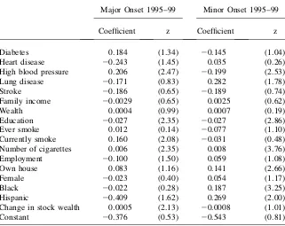
In all specifications, not surprisingly onsets of minor and major disease are strongly positively related to age and negatively related to baseline levels of self-assessed health status. Collectively, prior chronic conditions are also strong predic-tors of future new health onsets.10Smoking, and especially its intensity as proxied by the number of cigarettes, continues to produce new incremental bad health out-comes, even after conditioning on an extensive set of measures of current health Table 1
Probits Predicting Onsets of New Health Conditions—Baseline 1994
Major Onset 1995–99 Minor Onset 1995–99
Coefficient z Coefficient z
Age 51–61 0.420 (5.67) 0.355 (5.83)
Age 62-plus 0.809 (10.62) 0.331 (4.82)
Excellent health 20.315 (3.37) 20.424 (5.52)
Very good health 20.266 (3.29) 20.303 (4.42)
Good health 20.226 (2.98) 20.084 (1.31)
Arthritis 0.164 (2.22) 20.487 (6.50)
Cancer 0.048 (0.36) 20.341 (2.44)
Diabetes 0.240 (2.22) 20.192 (1.81)
Heart disease 20.296 (2.36) 0.238 (2.42)
High blood pressure 0.104 (1.47) 20.258 (3.98)
Lung disease 0.093 (0.68) 0.179 (1.52)
Stroke 0.130 (0.67) 20.255 (1.34)
Family income 20.0083 (1.78) 20.0054 (1.36)
Wealth 0.0005 (1.06) 0.0007 (1.58)
Education 20.016 (1.40) 20.017 (1.91)
Ever smoke 0.038 (0.48) 0.013 (0.21)
Currently smoke 0.229 (3.21) 20.100 (1.74)
Number of cigarettes 0.005 (2.24) 0.007 (3.39)
Employment 20.074 (1.21) 20.021 (0.43)
Own house 20.033 (0.52) 0.087 (1.81)
Female 0.028 (0.52) 0.062 (1.53)
Black 20.020 (0.27) 0.153 (2.90)
Hispanic 20.424 (1.85) 0.141 (1.19)
Change in stock wealth 0.0004 (1.26) 20.0010 (1.54)
Constant 21.011 (1.49) 20.056 (0.10)
Note: Models also control for Region of Residence and marital status and change in marital status between the waves.Zvalues are based on robust standard errors. Financial variables measured in $10,000 units.
Table 2
Probits Predicting Onsets of New Health Conditions—Baseline 1989
Major Onset 1990–94 Minor Onset 1990–94
Coefficient z Coefficient z
Age 51–61 0.448 (5.15) 0.572 (8.02)
Age 62 0.439 (4.13) 0.419 (4.72)
Excellent health 20.330 (2.71) 20.531 (5.45)
Very good health 20.220 (2.01) 20.333 (3.81)
Good health 20.042 (0.41) 20.218 (2.59)
Arthritis 0.122 (1.07) 20.434 (3.98)
Cancer 0.176 (0.87) 0.324 (1.77)
Diabetes 0.247 (1.61) 20.069 (0.45)
Heart disease 20.150 (0.82) 20.015 (0.10)
High blood pressure 0.127 (1.26) 20.232 (2.56)
Lung disease 0.395 (1.98) 0.275 (1.57)
Stroke 20.216 (0.62) 0.166 (0.65)
Family income 0.0049 (0.85) 0.0101 (1.79)
Wealth 20.0007 (0.80) 20.0028 (2.73)
Education 20.029 (2.25) 20.014 (1.31)
Ever smoke 20.029 (0.28) 0.176 (2.27)
Currently smoke 0.167 (1.93) 20.208 (2.90)
Number of cigarettes 0.010 (3.80) 0.001 (0.37)
Employment 20.189 (2.49) 20.001 (0.02)
Own home 0.041 (0.53) 0.207 (3.21)
Female 20.046 (0.69) 20.047 (0.89)
Black 20.378 (4.05) 0.125 (1.86)
Hispanic 20.288 (1.11) 0.098 (0.56)
Change in stock wealth 0.0009 (0.47) 20.0006 (0.33)
Constant 20.576 (0.92) 20.316 (0.46)
Major Onset 1995–99 Minor Onset 1995–99
Coefficient z Coefficient z
Age 51–61 0.546 (7.29) 0.194 (2.95)
Age 62 0.775 (8.77) 0.323 (4.03)
Excellent health 20.272 (2.69) 20.249 (2.91)
Very good health 20.283 (3.02) 20.189 (2.33)
Good health 20.069 (0.79) 20.022 (0.28)
Arthritis 0.136 (1.43) 20.581 (5.64)
Cancer 20.002 (0.01) 20.285 (1.42)
status. Because smoking has a strong negative gradient with education, its inclusion in these models reduces the predictive effects of education on new health onsets.
Whether one looks at the relatively short horizon of the next five years or a decade or more ahead, all three financial measures of SES—income, household wealth, and the stock market gains—are very poor predictors of future health outcomes whether they are major or minor onsets. The estimated coefficients are rarely statistically sig-nificant, and they even vacillate in sign being more often positive than negative. To illustrate, of the 36 coefficients estimated on the three financial variables (income, wealth, and new stock wealth) in Tables 1–3 in only four cases is the estimated effect statistically significant at the 5 percent level and in two of those four the effect is actually positive.
These longer horizon PSID results on financial measures of SES are quite power-ful in that they partly respond to the objection that one may have controlled for most of the indirect effects of SES by conditioning on baseline attributes including in-come. In this case, the conditioning variables are sometimes measured more than a decade before the disease onset. In sum, SES variables that directly measure or proxy for financial resources of a family are either not related or at best only weakly Table 2 (continued)
Major Onset 1995–99 Minor Onset 1995–99
Coefficient z Coefficient z
Diabetes 0.184 (1.34) 20.145 (1.04)
Heart disease 20.243 (1.45) 0.035 (0.26)
High blood pressure 0.206 (2.47) 20.199 (2.53)
Lung disease 20.171 (0.83) 0.282 (1.78)
Stroke 20.186 (0.65) 20.189 (0.74)
Family income 20.0029 (0.65) 0.0025 (0.62)
Wealth 0.0004 (0.99) 0.0007 (0.19)
Education 20.027 (2.35) 20.027 (2.86)
Ever smoke 0.012 (0.14) 20.077 (1.10)
Currently smoke 0.160 (2.08) 20.031 (0.48)
Number of cigarettes 0.006 (2.35) 0.008 (3.76)
Employment 20.100 (1.50) 0.059 (1.08)
Own house 0.083 (1.16) 0.141 (2.66)
Female 20.023 (0.40) 0.054 (1.17)
Black 20.022 (0.28) 0.187 (3.25)
Hispanic 20.409 (1.62) 0.269 (2.00)
Change in stock wealth 0.0005 (2.13) 20.0008 (1.01)
Constant 20.376 (0.53) 20.543 (0.81)
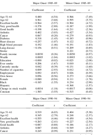
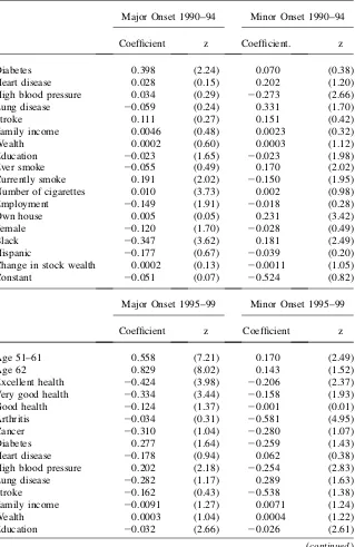
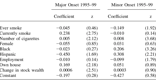
Table 3
Probits Predicting Onsets of New Health Conditions—Baseline 1984
Major Onset 1985–89 Minor Onset 1985–89
Coefficient z Coefficient z
Age 51–61 0.480 (4.54) 0.566 (7.49)
Age 62 0.561 (3.68) 0.595 (5.75)
Excellent health 20.564 (3.57) 20.504 (4.72)
Very good health 20.378 (2.88) 20.187 (1.99)
Good health 20.198 (1.64) 20.211 (2.36)
Arthritis 0.402 (3.03) 20.427 (3.34)
Cancer 0.067 (0.20) 20.279 (0.93)
Diabetes 0.318 (1.45) 20.183 (0.96)
Heart disease 20.257 (1.07) 0.122 (0.72)
High blood pressure 0.192 (1.46) 20.191 (1.83)
Lung disease 20.156 (0.51) 20.209 (0.89)
Stroke 0.221 (0.73)
Family income 0.0030 (0.26) 0.0050 (0.57)
Wealth 0.0005 (1.04) 0.0003 (1.02)
Education 20.000 (0.02) 20.025 (2.08)
Ever smoke 0.206 (1.67) 0.010 (0.11)
Currently smoke 0.042 (0.39) 20.131 (1.60)
Number of cigarettes 0.009 (2.93) 0.012 (4.72)
Employment 0.092 (0.87) 0.026 (0.39)
Own house 0.056 (0.56) 0.273 (3.66)
Female 20.080 (0.94) 0.111 (1.78)
Black 20.185 (1.55) 0.234 (2.98)
Hispanic 20.368 (1.57)
Change in stock wealth 0.0034 (1.18) 20.0017 (0.08)
Constant 21.585 (3.55) 20.515 (0.45)
Major Onset 1990–94 Minor Onset 1990–94
Coefficient z Coefficient. z
Age 51–61 0.519 (6.03) 0.404 (5.38)
Age 62 0.345 (2.79) 0.248 (2.37)
Excellent health 20.555 (4.46) 20.450 (4.54)
Very good health 20.263 (2.41) 20.227 (2.54)
Good health 20.087 (0.88) 20.186 (2.17)
Arthritis 0.087 (0.68) 20.549 (4.27)
Cancer 0.245 (0.99) 0.231 (0.95)
Table 3 (continued)
Major Onset 1990–94 Minor Onset 1990–94
Coefficient z Coefficient. z
Diabetes 0.398 (2.24) 0.070 (0.38)
Heart disease 0.028 (0.15) 0.202 (1.20)
High blood pressure 0.034 (0.29) 20.273 (2.66)
Lung disease 20.059 (0.24) 0.331 (1.70)
Stroke 0.111 (0.27) 0.151 (0.42)
Family income 0.0046 (0.48) 0.0023 (0.32)
Wealth 0.0002 (0.60) 0.0003 (1.12)
Education 20.023 (1.65) 20.023 (1.98)
Ever smoke 20.055 (0.49) 0.170 (2.02)
Currently smoke 0.191 (2.02) 20.150 (1.95)
Number of cigarettes 0.010 (3.73) 0.002 (0.98)
Employment 20.149 (1.91) 20.018 (0.28)
Own house 0.005 (0.05) 0.231 (3.42)
Female 20.120 (1.70) 20.028 (0.49)
Black 20.347 (3.62) 0.181 (2.49)
Hispanic 20.177 (0.67) 20.039 (0.20)
Change in stock wealth 0.0002 (0.13) 20.0011 (1.05)
Constant 20.051 (0.07) 20.524 (0.82)
Major Onset 1995–99 Minor Onset 1995–99
Coefficient z Coefficient z
Age 51–61 0.558 (7.21) 0.170 (2.49)
Age 62 0.829 (8.02) 0.143 (1.52)
Excellent health 20.424 (3.98) 20.206 (2.37)
Very good health 20.334 (3.44) 20.158 (1.93)
Good health 20.124 (1.37) 20.001 (0.01)
Arthritis 20.034 (0.31) 20.581 (4.95)
Cancer 20.310 (1.04) 20.280 (1.07)
Diabetes 0.277 (1.64) 20.259 (1.43)
Heart disease 20.178 (0.94) 0.062 (0.38)
High blood pressure 0.202 (2.18) 20.254 (2.83)
Lung disease 20.282 (1.17) 0.289 (1.63)
Stroke 20.162 (0.43) 20.538 (1.38)
Family income 20.0091 (1.27) 0.0071 (1.24)
Wealth 0.0003 (1.04) 0.0004 (1.22)
Education 20.032 (2.66) 20.026 (2.61)
related to the future onset of disease over the time span of 15 years.11These results imply that whether interpreted as predictions or more boldly as causally, financial measures of SES appear to have no discernable impact on future onsets of disease. As mentioned above, one explanation for the absence of any significant effects of the stock market variable on health is that there may be asymmetric effects during stock market upturns and downturns. To test this possibility, I estimated identical onsets models to the ones listed in Tables 1–3 for 1999–2001 and 1999–2003. The first years during this time period were years when the stock market experienced a sharp collapse, especially in tech stocks. The estimated effect of stock market gains and losses vacillated in sign and in no case was an estimatedzvalue on a stock mar-ket gain or loss variable higher than one. However, there is no reason to use only the 2001 or 2003 PSID to test this idea, a time horizon that may be too short to ade-quately capture any subsequent health effects. Even during periods characterized by large and pervasive capital gains, there are individuals who selected their portfo-lios badly and lost considerable money. A parallel argument applies during down-turns. I reestimated the models in Tables 1–3 separating out capital gains from capital losses and tested for impact of losses and gains separately. Once again, there were no statistically significant effects of either capital gains or capital losses on any future health onsets.
All this does not imply that at a more general level SES cannot predict future health events. Even within the contours of the models estimated in Tables 1–3, ed-ucation is mostly a statistically significant predictor of major health events across Table 3 (continued)
Major Onset 1995–99 Minor Onset 1995–99
Coefficient z Coefficient z
Ever smoke 20.045 (0.46) 20.149 (1.92)
Currently smoke 0.238 (2.75) 20.010 (0.14)
Number of cigarettes 0.005 (2.12) 0.008 (3.68)
Female 20.055 (0.85) 0.031 (0.63)
Black 20.023 (0.27) 0.206 (3.26)
Hispanic 20.450 (1.69) 0.308 (2.21)
Employment 20.010 (0.14) 20.099 (1.79)
Own house 0.169 (2.18) 0.051 (0.89)
Change in stock wealth 0.0006 (2.51) 0.0003 (0.90)
Constant 20.197 (0.28) 20.427 (0.58)
Note: Models also control for Region of Residence and marital status and change in marital status between the waves.Zvalues are based on robust standard errors. Financial variables measured in $10,000 units. NA means no coefficient estimated for that variable.
both a short- and long-term horizon. Even after one controls for an extensive array of baseline health and financial economic conditions, those with less schooling appear to be more likely to experience a major negative health onset. Of the 12 education coefficients estimated in these three tables, all are negative and eight are statistically significant at the 10 percent level of significance. This is true both over the short horizon of the next five years as well as over the longest horizon represented in the data—11–15 years out. The effect of education appears to become more statistically significant the longer the horizon allowed for the detection of the onset. Even after conditioning on all prior health events, themselves related to education, years of schooling still has predic-tive effects on diminishing the likelihood of a new health onset.
A legitimate issue about the models listed in Tables 1–3 is their reliance on single-period Markovs in both income and health. For several reasons, of which measure-ment error in either income or health would be but one good example, one-period Markovs are quite limited. Even without measurement error, current income may not be the appropriate concept for predicting future disease trajectories. Future onset of disease may be more influenced by longer-term measures of financial resources, which may well be one reason why education matters so much. Similarly, measures relying only on last period’s health ignore the duration dimension of any health prob-lems that might exist, a dimension quite likely to be associated with the onset of new disease. With this in mind, the models were reestimated using up to four-period in-come lags and four-period lags in self-reported general health status. The baseline 1984 model only would allow a Year 1 lag in general health status and a baseline 1994 would only permit a short window for a new onset to occur. Therefore, models with these longer lag structures in income and health were estimated for the 1989 baseline using a ten-year future horizon for the onset of a disease. All other covari-ates in these models remain the same as those in Tables 1–3.
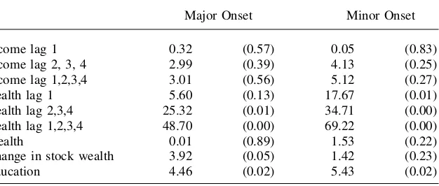
Because the principal issue is whether these lags matter, Table 4 summarizes the results with a series ofF-tests and the associated probabilities for differences from zero for a one-period lag, the three additional lags beyond the last year, and the
Table 4
Does SES Predict Future Major Onset with Lag Values of Income and Health? (F-tests and p values; 1989 Baseline—10 Year Forecast)
Major Onset Minor Onset
Income lag 1 0.32 (0.57) 0.05 (0.83)
Income lag 2, 3, 4 2.99 (0.39) 4.13 (0.25)
Income lag 1,2,3,4 3.01 (0.56) 5.12 (0.27)
Health lag 1 5.60 (0.13) 17.67 (0.01)
Health lag 2,3,4 25.32 (0.01) 34.71 (0.00)
Health lag 1,2,3,4 48.70 (0.00) 69.22 (0.00)
Wealth 0.01 (0.89) 1.53 (0.22)
Change in stock wealth 3.92 (0.05) 1.42 (0.23)
full four periods. The results obtained with lag structures on income are easy to summarize—in no case do any of the variants of the income lags matter. Since a four-period year should serve as a reasonable approximation to long-run measures of income, this suggests that the reason current income doesn’t matter does not lie in the familiar permanent-transitory income distinction. Moreover, the prior sum-mary that they also do not predict future onset for the other financial variables in-cluded in the model—wealth and the change in wealth—remains intact even with the full set of income and health lags in place. Finally, education still predicts future major and minor disease onset indicating that it is not simply serving as a proxy for permanent income, which should be adequately captured by the lag structure in past incomes.
The story for lagged health, however, is quite different. A one-period lag for health is clearly rejected and the full four-period lag structure is needed to predict future health onset. As mentioned above, this probably reflects both measurement error in health, especially in a noisy self-reported general health status (Crossley and Kennedy 2002), as well as the fact that these health lags pick up the impact of du-ration of illness. However, even that four-period structure does not alter the conclu-sion that even after conditioning on these measures of health over the last four years, education still predicts future onset and financial measures of SES do not.
One advantage of the PSID is that it allows us to investigate whether predictive effects of SES on health onset vary with age. Much current research on this topic is based either on the original HRS (Smith 1999) or the AHEAD cohort (Adams et al. 2003), which were originally restricted to those between the ages of 51–61 and 70-plus, respectively. To investigate this possibility, separate models were esti-mated over three age groups—those younger than 40, those older than 60, and those between those ages. While certainly less common than for people in the HRS and AHEAD age ranges, health episodes for PSID respondents who are younger than 50 years old are not negligible. For example, among those in their 40s in the 1999 wave, one in seven had previously experienced a major disease onset at some time in their lives and 40 percent have a minor chronic health condition. In the five years before 1999, 7 percent of these 40-year-olds experienced a major disease onset while one in four reported a new minor onset.
Sample sizes are necessarily much smaller when the models are estimated sepa-rately into these three age groups. This reduction in sample size becomes especially problematic when onsets are rare—that is the younger the sample (especially for the major onsets) and the shorter the duration over which one allows an onset to occur. Because of these considerations, I estimated onset models for these age group mod-els over ten-year horizons for the1984 and 1989 baseline year’s specifications and over the full 15-year horizon for the 1984 baseline model. With the exception of age, which is the stratifying variable, these models include the same set of covariates as in Tables 1–3.
wealth variable.12 Apparently, the ability of financial variables to predict future onsets is not sensitive to the stage of the adult life cycle one happens to be in.13
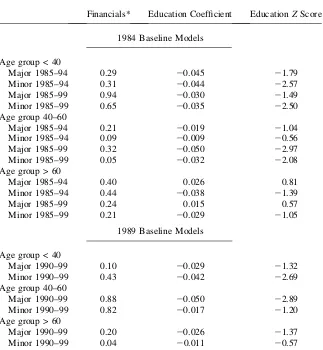
Table 5
Does SES Predict Future Onsets by Age?
Financials* Education Coefficient EducationZScore
1984 Baseline Models
Age group < 40
Major 1985–94 0.29 20.045 21.79
Minor 1985–94 0.31 20.044 22.57
Major 1985–99 0.94 20.030 21.49
Minor 1985–99 0.65 20.035 22.50
Age group 40–60
Major 1985–94 0.21 20.019 21.04
Minor 1985–94 0.09 20.009 20.56
Major 1985–99 0.32 20.050 22.97
Minor 1985–99 0.05 20.032 22.08
Age group > 60
Major 1985–94 0.40 0.026 0.81
Minor 1985–94 0.44 20.038 21.39
Major 1985–99 0.24 0.015 0.57
Minor 1985–99 0.21 20.029 21.05
1989 Baseline Models
Age group < 40
Major 1990–99 0.10 20.029 21.32
Minor 1990–99 0.43 20.042 22.69
Age group 40–60
Major 1990–99 0.88 20.050 22.89
Minor 1990–99 0.82 20.017 21.20
Age group > 60
Major 1990–99 0.20 20.026 21.37
Minor 1990–99 0.04 20.011 20.57
Note: This financial column reports thepvalue associated with the joint statistical significance for the coef-ficients for the three financial variables—income, wealth, and changes in stock market wealth. Models in-clude all variables inin-cluded in models in Tables 1–3. Using the minor onset models, sample sizes for the 1984 baseline were 2,788 (<age40), 1,388 (>40 and <60), and 374 (>60). The corresponding sample sizes for the 1989 baseline models were 2,972 (<age40), 1,744 (>40 and <60), and 678 (>60).
12. The sole exception is the 60-plus age group for the 1989 baseline where the stock market variable is statistically negative.
The remaining columns in Table 5 list estimated coefficients and associatedz val-ues for the education variable in each model. Data necessarily gets thinner with these age stratifications (especially in the oldest age group) and conclusions must be tempered. But for those in the two age groups ages less than 60 and younger, the con-clusion that education remains a strong predictor of future onset of disease appar-ently remains intact. This is far less apparent for the 60–plus age groups where the estimated effects of education are statistically significant. This is consistent with the findings of Adams et al. (2003) who used the AHEAD sample (aged 70-plus) and reported virtually no effects of any SES variables including education on subsequent health outcomes.
It may also reflect an inherent limitation of the PSID for research in this age group. The 1984 baseline estimates are especially problematic with this age stratifi-cation. The 60-plus population in 1984 would be aged 75-plus and living in 1999 when the questions on past disease onset were first asked. Very few people of that age who suffered a severe disease onset would still be alive in 1999, and they would be quite unrepresentative of the actual onsets that occurred. While somewhat less se-vere, as they would have to be only aged 70-plus in 1999, the same type of problem exists with the 1989 baseline models. This raises a more general point that the earlier years of the PSID for this type of analysis are probably best restricted to younger age groups.
Additional research on why education matters so much should receive high prior-ity. It is not simply due to education’s association with poor health behaviors. Smok-ing, perhaps the most important health behavior, is controlled for in this analysis, and other work with the HRS using more comprehensive health measures including smoking, drinking, and obesity show similar net impacts of education (Smith 2005). The basic source of the large estimated impact of schooling on success in many life domains, of which health is only one example, may be the most important unan-swered question in the social sciences. One possibility is that the education experi-ence itself has little to do with it, but is simply a marker for personal traits (reasoning ability, rates of time preference, etc.) that lead people to acquire more education and to be healthier. But education may not be that passive. It may help train people in decision-making, problem-solving, perseverance, and adaptive skills, all of which have direct applications to a healthier life. Education may have biological effects on the brain, which result in improved cognitive function and problem-solving abil-ity, some of which may impart benefits to choices made regarding one’s health. This is similar to the argument that more active brain functioning when younger pushes off the onset of dementia.
One approach to isolating such a causal path of schooling follows the lead of Lleras-Muney (2005) who provided evidence that laws affecting the age of school entry and the age at which a child could obtain a work permit significantly affected years of schooling completed during the 1915–39 period.14Lleras-Muney found sta-tistically significant effects of the component of schooling induced by compulsory schooling laws on subsequent mortality.
One difficulty with relying on this approach with the PSID is that those affected by such laws would be relatively older cohorts in the PSID, the very group identified above as not being PSID’s strong suit. A more promising approach may lie in appli-cations in other countries where the impact of such laws were larger and more recent. For example, England raised the statutory minimum from 14 to 15 shortly after the Second World War and again from 15 to 16 in 1974.
Cunha and Heckman (2006) instead emphasize the importance of cognitive and noncognitive skills such as motivation, persistence and self-control in explaining schooling and one’s eventual success in multiple domains of life. They see these skills as produced mainly by the family and by repetitive cumulative personal deci-sions whereby individuals teach themselves to do the right thing.
Whatever the source of the cognitive and noncognitive skills associated with ed-ucation, results presented here, and in related research, suggest that they are critical for improved health outcomes for several reasons. One is better self-management of disease. In a study using the DCCT clinical trial for Type 1 diabetes, Goldman and Smith (2002) found that the ability to comply with complex health regimens differed significantly between patients with high- and low-education levels, and that the differ-ence was a critical factor in successful glycemic control. Indeed, when low- and high-education patients were assigned to a group in which treatment regimens were strictly enforced, low-education patients showed a much more dramatic improvement in health outcomes. This indicates that less-educated patients might benefit from frequent fol-lowup, simpler drug regimens, and clearer instructions about how to comply.
In a subsequent study, Smith (2006) demonstrated that the high-education advan-tage with diabetes actually reflected three factors. At least in more recent years, the less-educated were of slightly higher risk in contracting the disease, consistent with the general findings in this paper. Second and much more important, the less-educated are at greater risk of having their diabetes undiagnosed and presumably un-treated. Third, even after diagnosis, the less-educated have considerable difficulty in successful disease management using the complex treatments necessary to diminish the negative health consequences associated with diabetes.
When diseases are not as complex as diabetes and treatment is more standard, these disparities by education tend to disappear. For example, Goldman and Smith (2005) examined the introduction of new drugs to treat hypertension, of which there have been several important examples over the last 25 years. They found no evidence that the diffusion of these new drugs into medical treatment favored one education group relative to another. This suggests that at least for hypertension, a key risk fac-tor for CHD, that SES differences in the adoption of new medical technologies are not an important reason for the SES-health gradient. In contrast, Lleras-Muney and Lichtenberg (2002) exploring a wider class of drugs that in general are more complex report that more educated individuals use drugs recently receiving FDA approval.
IV. Conclusions
ongoing SES-health debate. In this evaluation, I place emphasis on the possibility of using the retrospective information on incidence of chronic conditions. While noth-ing is perfect, the PSID passes this test with the principal issues benoth-ing that research-ers must take into account dating issues—especially the use of focal points. Analysis that allows for some relatively minor flexibility in the precise dating of events would be less subject to error. Especially for older persons in the sample, the data become less useful the further one goes back in time due to issues of mortality and attrition associated with the onset of health events, particularly the more severe ones. The quality of the dating of onsets appears to be more reliable when they refer to more severe events.
The paper also offers several substantive conclusions. First, across the life course, SES impacts future health outcomes, although the primary culprit appears to be ed-ucation and not an individual’s financial resources in whatever form they might be received. That conclusion appears to be robust to whether the financial resources are income or wealth or to whether the financial resources represent new information such as the largely unanticipated wealth that was a consequence of the recent stock market boom. Finally, this conclusion appears to be robust across new health out-comes that take place across the short and intermediate time frames of up to 15 years in the future.
Appendix 1 Quality of the PSID Health Data
The analysis in this paper relies heavily on the retrospectively col-lected health condition onset information colcol-lected during the 1999 wave of the PSID. Retrospective data have several well-documented issues surrounding the abil-ity to recall.15The extensive literature on this subject indicates that questions about events that occurred decades ago tend to yield a less reliable response than a query about a similar event taking place last week or last year. Similarly, the more salient an event the more likely it will be recalled, particularly as time since the event in-creases. Some studies have shown that event nonsalience is also associated with a tendency to report the event as having taken place more recently than it actually did (forward telescoping).
The key dimension of quality of PSID health information, especially for the type of analyses in this paper, concerns retrospective information on date of disease onset. A common problem with date recall involves an overreliance on focal responses, es-pecially easily remembered digits. When asked about the date of onset, respondents may center their responses on five, 10, 15, 20 years ago, etc.16Appendix Figures A and B document the extent of this problem by plotting the frequency distribution of year of onset for each chronic condition. Figure A illustrates four chronic condi-tions—arthritis, diabetes, high blood pressure, and diseases of the lung—where the
15. A large literature has developed on response errors in general and the quality of recall data in particular. Sudman and Bradburn (1974); Sudman, Bradburn, and Schwarz (1996); Bound, Brown, and Mathiowetz (2000); and Smith and Thomas (2003) provide insightful summaries.
problem appears to be most serious, while Figure B includes three diseases— cancer, stroke, and heart disease—where the use of focal values is less common. The tendency to concentrate responses on focal responses is far greater the less se-rious the disease and the further back in time the health event occurred. Concentra-tion on focal responses appears to be less for cancer than hypertension and greater at the 10-year point than at the five-year point.
All PSID questions including the 1999 health battery are answered by one respon-dent who reports for him/herself and the spouse, if any. It is reasonable to suspect Figure A
that the accuracy of reports may be better when the information requested refers to the respondent than when a respondent is asked about the spouse. Appendix Table A1 investigates this issue by listing the fraction of cases where disease onset was reported five or 10 years ago or 15 or 20 years ago. This data are stratified by whether the onset was major or minor and whether the report was about the respondent or spouse. Following the analysis in this paper, major conditions were defined as cancer, heart condition, stroke, and diseases of the lung. All other onsets are defined as minor.17
For recent events, say around the five- or 10-year marker, where the event is likely to be remembered but the date is uncertain, one would anticipate more focal year responses when the onset refers to the spouse instead of the respondent. This ten-dency should be greater for minor health onsets than for major ones. Appendix Table A1 supports both conjectures—27 percent of all minor onsets for the spouse are reported at a five-year or 10-year interval compared to 23 percent for the respondent. Figure B
Date of Onset of Chronic Condition (2)
The difference for major onsets is much smaller—17.8 percent compared to 16.7 percent.
In contrast, when the event took place in the distant past, say around the 15- or 20-year marker, remembering the event at all is at risk, especially for the spouse where the health event may have even preceded the marriage date. The greater tendency to not remember the event for spousal onsets could overwhelm the greater concentra-tion at focal years. Appendix Table A1 supports this conjecture. For health events taking place more than 10 years ago, there is a greater concentration at focal years for self-health onsets than there are for spousal onsets.
A useful comparison to assess data quality would involve the same type of infor-mation for people of the same age collected at the same time prospectively. Surveys like the HRS that have been collecting information prospectively for over a decade presumably should serve as a useful quality benchmark for the retrospective PSID onset data as the uncertainly over timing may be largely (but not completely) con-fined to a two-year window.
Appendix Table A2 documents the extent of onset of new health events that took place across the first five waves of the HRS—an eight-year time interval. In the left side of the panel, these onsets represent incidence rates for major and minor chronic conditions for respondents who were members of the original HRS cohort (those born between 1931 and 1941) in 1992 (approximately 51–61 years old).
The extent of the new health problems reported in HRS during these eight years is impressive. About half of all respondents experienced some type of onset during the first five HRS waves. The conditional probability of a major onset is much higher if one had already reported some type of health problem at HRS baseline than if one was chronic condition free. Appendix Table A2 attempts to replicate the same in-formation retrospectively from the PSID in the right side panel. Since the chronic conditions information is first available in 1999, the sample used to maintain com-parability with HRS are those PSID respondents who were 59–69 years old in that year and who would have been 51–61 years old in 1991. Using the PSID prevalence Appendix Table A1
Focal Point Responding for Self and Spouse (Percent Reporting at Focal Years)
Focal Point Years
5–10 11,15
Minor onset
Spouse 27.2 12.8
Self 22.7 15.1
Major onset
Spouse 17.8 5.9
Self 16.7 8.5
and year of onset data available, 1991 prevalence rates and the extent of new onset over the next eight years were computed—the same time frame used for the HRS in Appendix Table A2.
When we examine incidence across these eight years, minor incidence is actually higher in the PSID compared to the HRS. This ranking may indicate some forward telescoping of minor conditions in terms of date of onset in the PSID, a not uncom-mon finding with less salient events. In contrast, the two surveys are almost identical in the reporting incidence of major conditions. This data suggest that the timing data in the PSID may be more reliable for the major onset conditions with more serious recall issues for the minor onsets.
These issues related to recall bias suggest several points to keep in mind in the analyses in this paper. First, any dating reporting problems are much less important for major chronic conditions than for minor ones. Second, health onsets that took place close to 1999 should be less affected by recall bias so that quality of estimates of the impact of health events may decay as we move the time interval back in time. Third, the bias may be less important for analysis where health onsets are the out-comes studied (as in this paper) than when we are attempting to measure their impact and place them on the RHS of the analysis. Fourth, by allowing some relatively mi-nor flexibility in the dating of events one can mitigate the impact of any reporting bias. For example, by extending the year prior to and after the reported time of onset, Appendix Table A2
Prospective Incidence in the Original HRS Cohort and Retrospective Incidence in the PSID Cohort
Original HRS PSID Cohort
Conditional Incidence Incidence Conditional Incidence Incidence
NONE 49.9 43.8
None 47.8 43.8
Minor 36.4 40.4
Major 15.5 15.8
MINOR 28.9 35.8
None 51.6 43.7
Minor 22.1 28.8
Major 26.5 27.5
MAJOR 21.4 20.4
None 50.3 44.4
Minor 28.9 31.8
Major 21.9 23.8
Source: Calculations by author from first five waves of HRS—sample born between 1931–41.
the probability that the health onset occurred within that interval appears to be sig-nificantly increased. This is the strategy pursued in this paper.
References
Adams, Peter, Michael Hurd, Daniel McFadden, Angela Merrill, and Tiago Ribeiro. 2003. ‘‘Healthy, Wealthy, and Wise? Tests for Direct Causal Paths Between Health and Socioeconomic Status.’’Journal of Econometrics112(1):3–56.
Bound, John, Charles Brown, and Nancy Mathiowetz. 2000. ‘‘Measurement Error in Survey Data,’’ Research Report No. 00-450, Population Studies Center. Ann Arbor: University of Michigan.
Case, Anne, and Angus Deaton. 2005. ‘‘Broken Down by Work and Sex: How our Health Declines.’’ InAnalyses in the Economics of Aging, ed. David Wise, 185–212. Chicago: University of Chicago Press.
Case, Anne, Darren Lubotsky, and Chris Paxson. 2002. ‘‘Economic Status and Health in Childhood: The Origins of the Gradient.’’American Economic Review92(5):1308–34. Case, Anne, Angela Fertig, and Christina Paxson. 2005. ‘‘The Lasting Impact of Childhood
Health and Circumstance.’’Journal of Health Economics24:365–89.
Cunha, Flavio, and James J. Heckman. 2006. ‘‘Investing in our Young People.’’ Unpublished paper prepared for Festschrift in honor of Professor Robert Fogel,Economic Causes and Consequences of Population Aging.
Crossley, Thomas, and Stephen Kennedy. 2002. ‘‘The Reliability of Self-assessed Health Status.’’Journal of Health Economics21(4):643–58.
Currie, Janet, and Rosemary Hansen. 1999. ‘‘Is the Impact of Health Shocks Cushioned by Socioeconomic Status.’’American Economic Review89(2):245–50.
Deaton, Angus. 2003. ‘‘Health, Inequality, and Economic Development.’’Journal of Economic Literature41(1):113–58.
Evans, William, Helen Level, and Kosali Simon. 2000. ‘‘Data Watch: Research Data in Health Economics.’’Journal of Economic Perspectives14(4):203–16.
Friedman, Milton. 1957.A Theory of the Consumption Function.Princeton: Princeton University Press.
Goldman, Dana, and James P. Smith. 2005. ‘‘Socioeconomic Differences in the Adoption of New Medical Technologies.’’American Economic Review95(2):234–37.
———. 2002. ‘‘Can Patient Self-Management Help Explain the SES Health Gradient?’’ Proceedings of the National Academy of Sciences99(16):10929–34.
Lleras-Muney, Adriana. 2005. ‘‘The Relationship Between Education and Adult Mortality in the U.S.’’Review of Economic Studies72 (1):189–221.
Lleras-Muney, Adriana, and Frank Lichtenberg. 2002. ‘‘The Effect of Education on Medical Technology Adoption: Are the More Educated More Likely to Use Drugs.’’ NBER working Paper No. 9185. Cambridge: National Bureau of Economic Research.
Marmot, Michael. 1999. ‘‘Multilevel Approaches to Understanding Social Determinants,’’ in Social Epidemiology, ed. Lisa Berkman and Ichiro Kawachi, 349–67. Oxford: Oxford University Press.
Smith, James P. 2006. ‘‘Diabetes and the Rise of the SES Health Gradient.’’ Paper prepared for Festschrift in honor of Professor Robert Fogel,Economic Causes and Consequences of Population Aging.
———. 2005. ‘‘Consequences and Predictors of New Health Events,’’ inAnalyses in the Economics of Aging, ed. David A. Wise, 213–37. Chicago: University of Chicago Press. ———. 1999. ‘‘Healthy Bodies and Thick Wallets.’’Journal of Economic Perspectives
Smith, James P., and Duncan Thomas. 2003. ‘‘Remembrances of Things Past: Test-Retest Reliability of Retrospective Migration Histories.’’Journal of the Royal Statistical Society, 166(1):23–49.
Steptoe, Andrew, and Michael Marmot. 2004. ‘‘Socioeconomic Status and Coronary Heart Disease: A Psychobiological Perspective.’’ Aging, Health, and Public Policy: Demographic and Economic Perspectives.Population and Development Review.30(Supp.):133–50. Sudman, Seymour, and Norman Bradburn. 1974.Response Effects in Surveys: A Review and
Synthesis.Chicago: Aldine Publishing Company.