STRAIGHT-LINE PATH FOLLOWING IN WINDY CONDITIONS
A. Brezoescu∗, P. Castillo and R. Lozano
Heudiasyc Laboratory, UTC-CNRS 6599, Compiègne, France
(cbrezoes, castillo, rlozano)@hds.utc.fr
Commission WG I/V
KEY WORDS:UAVs, Flight planning, Flight performance, Wind disturbance, Control law
ABSTRACT:
A straight-line following controller for a small and light airplane flying in windy conditions is proposed. In a first time, the lateral dynamics of the plane are derived and the error deviation velocity with respect to the desired trajectory is computed. A simple nonlinear control law is developed in order to impose a linear behavior for the airplane position and to track the desired trajectory. Several simulations, taking into account quasi-constant wind disturbances, are performed to analyze the performance of the closed-loop system. Improved results are obtained including the airplane orientation to counter the wind as an input for the flight planning. In order to validate the proposed control scheme an airplane has been developed based on the classic aerodynamic layout. Future work will introduce the experimental results when applying in real-time the proposed control algorithm.
1 INTRODUCTION
The Unmanned Aerial Vehicles (UAVs) represent a lightweight solution designed for applications requiring low-altitude surveil-lance and reconnaissance intelligence. Also, they are best suited to solve dangerous situations and to perform rescue missions since they do not have a human pilot on board. Especially, since it is necessary for UAVs to fly at low altitude in order to observe ter-rain, UAVs are likely to face a danger to fall down because of irregular wind or obstacles. With advances in flight control and miniaturization of UAVs, they are found to play a key role in ur-ban environments. Most of the mission paths can be defined using a set of way-point and loiters maneuvers, where way-points are straight line segments while loiters are circular orbits. The path following controller has to accurately track the desired path in presence of wind disturbances. In addition, the path following control algorithm must have low computational complexity for use in small and large UAVs without any changes.
Automatic control for airplanes has a long history and these many control techniques are also able to be applied for autonomous UAVs. Since dynamics of airplanes are nonlinear, controllers based on linear theories are not sufficient for trim conditions which are different from the nominal trim condition. In order to over-come this difficulty, it is common to adopt robust and nonlinear control approaches, gain scheduling techniques and so on. For example, in (Rysdyk, 2006) the author develops a guidance law for UAVs to follow straight line, curved trajectories and loiter ma-neuvers in the presence of winds. Indeed in this paper, the authors introduce a path following approach called "good helmsman" for autonomous monitoring of a target. The approach uses a Serret-Frenet formulation to represent the vehicle kinematics in terms of path parameters. The UAV is brought from current path to the de-sired path by simultaneously regulating the cross track error and course angle error to zero in the Serret-Frenet frame. An observer estimates wind data, which is used to orient path geometry about the target.
A simple path following controller for small UAVs based on the concept of vector fields is presented in (Nelson et al., 2007).
∗Corresponding author
The controller generates desired course input in presence of con-stant wind disturbances and it provides asymptotic following for straight-line and circular paths. A sliding mode controller is used to bring the vehicle to follow the vector field. Another vector field approach is proposed in (Frew and D.Lawrence, 2008). Here, the authors guide the UAV to fly in a circular orbit around a target. The Lyapunov guidance vector field is first designed for a sta-tionary target in the absence of wind, and then a modified ver-sion of vector field is applied to the case with a moving target in known constant background wind. Only variable heading rate control input is used to achieve standoff tracking with a constant commanded airspeed. However, the estimation approach for un-known target motion and wind is not taken into account in this paper. Lyapunov vector fields approach was also used for coor-dinated standoff tracking of stationary or moving targets in UAV formations using a rigid graph theory, see for example (Summers et al., 2009).
In (Zhu et al., 2009) the authors have proposed an adaptive es-timation strategy to estimate the velocities of the unknown wind and target motion. In the proposed approach, a variable heading rate controller is designed to achieve standoff tracking of mov-ing target. On the other hand, a guidance law for a micro aerial vehicle, MAV, taking wind into consideration was designed by (Ceccarelli et al., 2007) for the purpose of continuous monitoring of a target in the camera field of view.
2 PROBLEM STATEMENT
The most common parameters involved in the UAV control prob-lem are: velocity, altitude, turn rate, flight-path angle, atmospheric turbulence. In this article we deal with the tracking problem of an airplane flying in presence of crosswind. Thus, the mission of the airplane will be to follow a desired trajectory whilst its performance may be modified by the wind. This problem be-comes more complex when considering the complete dynamics of the airplane, and in order to simplify analysis and to better understand the problem, hereafter we will focuss to study the lat-eral dynamics, i.e., the altitude and the pitch and roll angles are quasi-constant (stabilized).
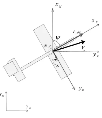
Figure 1: Forces and moments acting on the airplane
Therefore and from Figure 1, the nonlinear dynamic equations for the lateral flight take the form:
˙
u = X
m+rv (1)
˙
v = Y
m−ru (2)
˙
xN = ucosψ−vsinψ (3)
˙
yE = usinψ+vcosψ (4)
˙
r = IxxN
IxxIzz−Ixz2 (5) ˙
ψ = r (6)
whereuandvdenotes the airspeed components in the planeXB andYBrespectively,mis the mass of the plane,ψrepresents the yaw angle,rdescribes the yaw rate whileNthe yawing moment,
XandY are the forces due to aerodynamic effects and to engine thrust,Ijjsignifies the inertia component in thejaxis. The in-ertial frame is composed byXNandYEdenoting the position in thexaxis (North) and in theyaxis (East).
Considering a symmetrical airplane with a rigid spinning rotor placed in the front of its body, it can then be considered, without loss of generality,Vaacting only in thex-axis, see Figure 2. Then the following expressions can be stated
u ≈ T−D (7)
v << 1 (8)
Figure 2: Forces and moments acting on the airplane when con-sideringv <<1.
whereT is the thrust produced by the rotor andD is the drag force. Thus,
˙
xN ≈ (T−D) cosψ=Vacosψ ˙
yE ≈ (T−D) sinψ=Vasinψ
In real conditions, the plane is generally exposed to wind. If the airplane is experiencing a crosswind, it will be pushed over or yawed away from the wind. Let consider in this study a lateral wind having north and east velocity components,WN,WE re-spectively, see Figure 3. Hence the velocity in thecgof the air-craft with respect to the air and related in the body fixed frame is given by (Etkin, 1972):
vBE=vB+BB
WN
WE
(9)
wherevE B =
uE vET
is the aircraft speed relative to the air-mass in which it is flying expressed in body frame,vB = [u v]T describes the airspeed vector in body frame andBBdenotes the complete transformation from the inertial frame to the body frame
assuming zero roll and pitch angles, and it is given by
When equation 9 is added to the nonlinear equations of motion, thenvE
B, rather thanvB, must be used in the calculation of veloc-ity and orientation of the airplane. To track the flight path relative to Earth we need the velocity components in the directions of the axes of Earth fixed frame. We get these by expressing the velocity vectorvE
B in Earth frame (Stevens and Lewis, 1992). The differ-ential equations for the coordinates of the flight path are then
Therefore, the nonlinear equations representing the airplane move-ments in the planex-yand in presence of lateral wind becomes
˙
Hence, introducing the above into (11) and (12) and using (7) and (8), it follows that andψωdescribes the wind direction.
Figure 4: Tracking formulation problem
Remember that the control goal is that the airplane follows a desired trajectory with a constant airspeedValike in Figure 4. To simplify the analysis, let assume that the desired trajectory is aligned with the North axe of the reference frame, then, the de-sired path angle, represented in Figure 4 byψd, is equal to zero. Therefore, the amount of the trajectory deviation will depend on the velocity of the airplane and wind and also on the angle of the wind in relation to the airplane. Thus, the control corrections must be computed in order to reduce the error position,d, while controlling the variation of the yaw angle.
Thus, without loss of generality the following equation can be defined:
˙
d≡y˙E=usin(ψ) +ωsin(ψω) (13)
Note that the airplane yaw angle is referred to be the direction that the aircraft nose is pointing while the flight path angle is between the direction of flight and the compass reference (e.g., north), also known as heading.
3 GUIDANCE LAW DESIGN
Remember that the crosswind deflects the airplane from its orig-inal course. Consequently, it is necessary to point away from the intended course to counteract this effect. Therefore, the proposed guidance law will converge the position error to zero and the yaw angle to the absolute value of the wind correction angle. To this end, the yaw angle will be considered having two components: the component to minimize the position error,ψe, and the com-ponent to counter the wind,ψc, i.e.,
ψ=ψe+ψc (14)
Consider, in a first time, the airplane aligned with the desired trajectory with the position error very small, thus,ψe ≈ 0and
˙
For simulations purposes, let assume that the wind velocity and the wind orientation are constant. Remember also that the air-plane is flying with a constant speedVa≈uin a plane as shown
in Figure 4. Thus, from(13), we obtain
˙
d=usin(ψ) +kω (16)
wherekωis constant, see (13) and (15).
Notice that the above equation is relatively proportional to the variation of the yaw angle and it can be controlled using the rud-der of the airplane. The rudrud-der of the plane can be operated using the servo motor angular acceleration. Then, taking the second and third derivate with respect to the time from (16) and using (5) and (6), it follows that
Proposing
JN= ˙ψ2tanψ−3 ˙ψ− 3 ˙d+d
ucosψ (18)
then, the closed-loop system becomes ...
d =−3 ¨d−3 ˙d−d
ors3+ 3s2+ 3s+ 1 = 0, that represents a stable polynomial. Then from the above, it follows thatd(i)→0fori= 0,1,2,3.
4 SIMULATION RESULTS
A previous analysis of the nonlinear model is presented for dif-ferent conditions (with and without wind). Figure 5 introduces the behavior of the plane without wind whilst Figure 6 illus-trates the states affected by the wind. In this case we consider a crosswind having North and East velocity components ofWN =
1m/s, WE = 3m/srespectively. The values parameters are shown in Table 1. Notice from Figure 6 that the body-axis com-ponents of inertial velocity and the sideslip angle are presented.
Figure 5: Earth-Relative Aircraft Location
Meaning Value Airplane Velocity 20m/s
Airplane Orientation 0◦ Wind Velocity 0m/s
Altitude 200m
Table 1: Flying parameters without wind
Figure 6: Airplane states in presence of wind
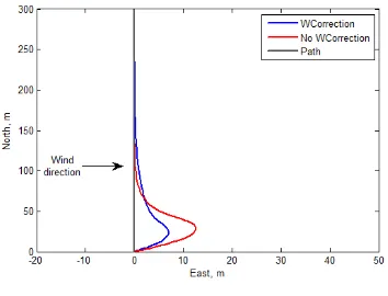
The proposed control strategy is validated in closed-loop system in simulations with various wind conditions. The UAV airspeed is considered 20 m/s while the wind velocity is 14 m/s. There is no initial path deviation and the wind direction is North-East perpendicular to the desired path, see Figure 7. The resulting trajectories in figures are plotted with blue line for Wind Cor-rection Controller (WCC) and red line for No Wind CorCor-rection Controller (NWCC).
Figure 7: Airplane response in presence of wind
Notice also from Figure 7 that the error using the WCC is 7.5 m while employing the NWCC this error is highly affected by cross-wind diverting almost 13 m from the path. In order to compare the performance of the two controllers we vary the wind speed magnitude and the wind orientation. In Figure 8, we illustrate the state responses for wind values of 1 m/s, 6 m/s and 11m/s while the wind blows perpendicular to the desired path. On the other hand, changing the wind orientation while keeping a con-stant wind velocity of 11 m/s, also results in a perturbed system, see Figure 9.
For comparative studies we plot, in Figures 10 and 11, the re-sults obtained employing the NWCC. The controller is affected by crosswind since it deviates more from the desired trajectory. The different wind magnitudes used to simulate the performance of the controller are 1 m/s, 6 m/s and 11 m/s respectively. Ob-serve in these figures that the controller shows good performance when considering the airplane orientation to counter the wind.
Figure 9: Earth relative position for different wind orientation
Figure 10: Position error reponse when using the No Wind Cor-rection Controller - NWCC
Figure 11: Earth relative position for different wind orientation
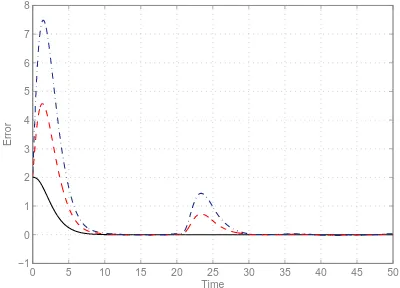
For the following simulations we assumed that the wind is char-acterized by constant velocity but it increases its speed during the flight. The wind velocity is plotted in Figure 12. If we have the knowledge about the wind parameters, we can compute the wind correction angle and the airplane will remain closer to the desired path. The positions errors are plotted in Figure 13 and 14 for different wind conditions. The parameters values used in this simulations are summarized in Table 2.
Once more we can notice a better performance of the controller
0 10 20 30 40 50
6.5 7 7.5 8 8.5 9 9.5
Time
Speed[m/s]
Figure 12: Wind velocity
Symbol Meaning Value
v Airplane Velocity 20m/s d0 Initial Error 2m
ω Wind Velocity 7m/s ψω Wind Orientation 0◦,45◦,90◦,180◦
Table 2: Control parameters
0 5 10 15 20 25 30 35 40 45 50 −0.5
0 0.5 1 1.5 2 2.5 3 3.5 4 4.5 5
Time
Error
Figure 13: Position error using WKC with different conditions of wind orientation:ψω= 0◦, ψω= 30◦, ψω= 90◦
0 5 10 15 20 25 30 35 40 45 50 −1
0 1 2 3 4 5 6 7 8
Time
Error
Figure 14: Position error using NWKC with different conditions of wind orientation:ψω= 0◦, ψω= 30◦, ψω= 90◦
5 AIRPLANE CONFIGURATION
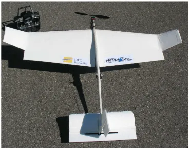
In this section we introduce briefly the airplane which we devel-oped in order to validate the proposed control law. Its configu-ration is based on the classic aerodynamic layout and it is built of polystyrene foam sheet and carbon fiber tubes. The airplane is powered by a brushless motor placed in front of the body. The airplane has five wings, a main airfoil-shaped wing fixed to the body, a couple of ailerons, an elevator and a rudder. Servo mo-tors are attached to ailerons, the elevator and the rudder as control surface actuators. Parameters of this airplane are given in Table 3 and a photo of the airplane is presented in Figure 15.
Parameter Value Airfoil Shape NACA Wing chord (¯c) 0.23m−0.19m
Wing span (b) 1.4m
Aspect ratio (AR) 6.49
Wing Area (s) 0,302m2
Mass Vehicle (kg) 0.70kg
Length (m) 1m
Table 3: Parameters of the airplane.
The airplane is able to take off from a runway and to land on the ground. The on-board computer system is the RabbitCore RCM4300 Microprocessor and it is connected to an airspeed and altitude sensor, and a Futaba system for a servo signal genera-tor/receiver unit. Sensor unit consists of three accelerometers, three gyroscopes and a magnetometer. All servo motors are con-trolled manually via radio control in manual mode, or automati-cally by an on-board computer system in auto mode.
Figure 15: The airplane prototype.
6 CONCLUSION
In this paper, a trajectory following controller for a small and light airplane flying in windy conditions was proposed. In order to achieve it, the lateral dynamic of the vehicle and the equation of the position deviation velocity with respect to the desired path were derived.
Some hypothesis have been stated in order to simplify the prob-lem and the analysis and a simple control law was proposed to tracking a desired trajectory. In addition, the proposed control law imposes a linear behavior for the airplane position and it has shown a good performance in simulations.
Improved results have been obtained including the airplane ori-entation to counter the wind as input for the flight. Therefore, the
position error remains small for small variations of wind param-eters.
The simulation results justify the reliability and efficiency of the proposed control law even considering the wind velocity variable. An airplane has been developed based on the classic aerodynamic layout having a unibody fuselage with wings providing majority of the lift. Future work will be done validating the proposed con-trol strategy in the prototype.
REFERENCES
Ceccarelli, N., Enright, J. J., Frazzoli, E., Rasmussen, S. J. and Schumacher, C. J., 2007. Micro uav path planning for reconnais-sance in wind. American Control Conference pp. 5310–5315.
Etkin, B., 1972. Dynamics of atmospheric flight.
Frew, E. and D.Lawrence, 2008. Cooperative standoff tracking of moving targets using lyapunov guidance vector fields. AIAA Journal of Guidance, Control, and Dynamics 31(2), pp. 290–306.
Nelson, D. R., Barber, D. B., McLain, T. W. and Beard, R. W., 2007. Vector field path following for small unmanned air ve-hicles. IEEE Transactions on Robotics and Automation 23(3), pp. 519–529.
Rysdyk, R., 2006. Unmanned aerial vehicle path following for target observation in wind. Journal of Guidance, Control, and Dynamics 29(5), pp. 1092–1100.
Stevens, B. L. and Lewis, F. L., 1992. Aircraft control and simu-lation.
Summers, T. H., Akella, M. R., and Mears, M. J., 2009. Co-ordinated standoff tracking of moving targets: Control laws and information architectures. Journal of Guidance, Control, and Dy-namics 32(1), pp. 56–69.