Employment of Single Mothers
Erdal Tekin
a b s t r a c t
This paper develops and estimates a model for the choice of part-time and full-time employment and the decision to pay for childcare among single mothers. The results indicate that a lower childcare price and a higher full-time wage rate both lead to an increase in overall employment and the use of paid childcare. The part-time wage effects are found to be too small to have significant behavioral implications. An analysis of cost-effectiveness indicates that the additional hours of work generated per dollar of government expenditure is larger for a childcare subsidy than a wage subsidy.
I. Introduction
The Personal Responsibility and Work Opportunity Reconciliation Act (PRWORA) of 1996, commonly known as welfare reform legislation, marks a cornerstone in U.S. welfare policy. Among the main goals of the PRWORA are to increase employment and to reduce welfare dependence among the low-income pop-ulation. In order to facilitate the transition from welfare to work and help low-income families maintain economic self-sufficiency, the new law streamlined the childcare assistance system by consolidating four main childcare subsidy programs into a sin-gle block grant, the Child Care Development Fund (CCDF).1 Under the new law, states are given unprecedented flexibility to design and implement their own child-care assistance programs. Furthermore, states are allowed to transfer up to 30 percent
Erdal Tekin is an assistant professor of economics at the Andrew Young School of Policy Studies at Georgia State University, a faculty research fellow at NBER, and a research fellow at IZA. The author thanks David Blau, Naci Mocan, Thomas Mroz, David Ribar, Paula Stephan, and seminar participants at University of North Carolina at Chapel Hill, Tulane University, Georgia State University, Urban Institute, Research Triangle Institute (RTI), and the Institute for the Study of Labor (IZA) in Germany for helpful comments and suggestions. The author is also grateful for research support from the Child Care Bureau and the UPS Foundation. The data used in this article can be obtained beginning October 2007 through September 2010 from Erdal Tekin, P.O. Box 3992, Atlanta, GA 30302-3992 tekin@gsu.edu
[Submitted August 2005; accepted August 2006]
ISSN 022-166X E-ISSN 1548-8004Ó2007 by the Board of Regents of the University of Wisconsin System
T H E J O U R NA L O F H U M A N R E S O U R C E S d X L I I d 2
of their Temporary Assistance to Needy Families (TANF) funds into the CCDF and to directly spend additional TANF funds for childcare assistance. These changes have placed childcare at the center stage of the welfare reform debate. As a result, total expenditures on childcare have increased substantially since the passage of PRWORA. For example, total CCDF expenditures rose by 84 percent, from about $4.4 billion to about $8.1 billion, between 1997 and 2001. In 2003, total expenditures from federal and state funds reached around $9.3 billion, which served approxi-mately 1.75 million children on average every month (Besharov and Hihney 2006). The goal of this paper is to examine the effects of the price of childcare and wages on the part-time and full-time employment decision, as well as the decision to use paid childcare among single mothers. Although it is well documented in the literature that the cost of childcare serves as a deterrent to the employment of mothers, there is little consensus on the size of the childcare price elasticity of employment. There-fore, it is important to provide new evidence that would help resolve this uncertainty. The majority of the early studies on this issue focus on married mothers. Although researchers have recently started to focus on samples of single mothers or have con-ducted analyses separately for married and single mothers, our knowledge on the responses of single mothers to the price of childcare is still limited. Given the recent legislative changes aimed at increasing employment among the low-income popula-tion, of whom single mothers are overrepresented, more insights are needed on the responses of single mothers to wages and the price of childcare.2
There is a relatively large literature on the effect of childcare prices on the em-ployment of mothers. However, most studies use data that predate welfare reform and other important policy changes of the early and mid-1990s. The empirical anal-ysis in this paper is a step forward because it uses a data set that was collected after these changes.3This paper also adds to the literature by incorporating the childcare subsidy receipt decision into the mother’s choice set along with the employment and childcare mode decisions. Another contribution of the present paper is that it treats the market price of childcare differently between subsidy recipients and nonreci-pients by implementing an adjustment to the price of childcare by the amount of the subsidy for those mothers who receive one. This may be important because the price of childcare faced by subsidy recipients is different from those faced by nonrecipients, and mothers respond to the childcare price net of subsidy when mak-ing their employment decision. Blau and Tekin (forthcommak-ing) and Meyers, Heintze, and Wolf (2002) examine the effect of actual subsidy receipt on the binary employ-ment decision of mothers, accounting for the endogeneity of subsidy receipt. How-ever, this paper is the first study to incorporate the childcare subsidy receipt into the choice set of employment and childcare payment decisions.
The majority of the studies in the childcare literature consider the binary employ-ment decision. Exceptions include Powell (1998), Connelly and Kimmel (2003b), Michalopoulos and Robins (2000) who distinguish between the part-time and full-time employment decision (similar to this paper), and Michalopoulos, Robins, and Garfinkel (1992), Powell (1997) and Averett, Peters, and Waldman (1997) who esti-mate hours of work equations. Distinguishing between part-time and full-time work may be important as childcare utilization is likely to differ between the two markets due to different attractiveness and transaction costs (Connelly and Kimmel 2003b). This paper also allows for the wage rate to be determined separately for part-time and full-time workers and distinguishes between part-time and full-time wage rates. One of the main goals of welfare reform is to reduce welfare dependence and increase employment. Therefore, policies designed to raise the effective wage rate also would be considered as a tool for this objective in addition or as an alternative to childcare subsidies. In order to fully understand the effectiveness of different policy options, it is important to examine the effect of wages on single mothers’ employment decision. This paper develops and estimates a behavioral model for the choice of part-time and full-time employment and the decision to pay for childcare among single moth-ers, using data from the 1997 National Survey of America’s Families (NSAF). A multinomial choice model for the discrete decisions of employment, childcare pay-ment, and childcare subsidy receipt are estimated jointly with the continuous wage equations for part-time and full-time employment and the price of childcare.
The results show that both the price of childcare and the wage rate affect the behavior of single mothers in the ways predicted by economic theory. That is, a de-crease in the price of childcare inde-creases employment and the use of paid child-care, and an increase in the full-time wage rate raises both overall employment and the use of paid childcare. Furthermore, the effect of the part-time wage rate on employment is found to be much smaller than the effect of the full-time wage rate. The results also indicate that single mothers who are employed full-time are more sensitive to the price of childcare than those who are employed part-time. The elas-ticity of employment with respect to the full-time wage rate is found to be larger than both the part-time wage elasticity of employment and the childcare price elasticity of employment. However, the cost-effectiveness, as measured by the additional number of hours of work generated per dollar of government expenditure, is found to be larger for a childcare subsidy than a wage subsidy.
The remainder of the paper is organized as follows. Section II provides a literature review. Section III discusses the theoretical model and the econometric approach. Section IV describes the data set. Section V reports the empirical results. Section VI presents the concluding remarks and the policy implications.
II. Literature Review
and Robins 1991; Michalopoulos, Robins, and Garfinkel 1992) to a high of 21.26 (Hotz and Kilburn 1994), with some clustering between20.3 and20.4. The studies differ in data sources, sample compositions, specifications, and estimation methods. However, sample compositions and data sources alone are unlikely to account for much of this wide variation because the range of estimates is large even within stud-ies using the same data set and similar sample compositions (Kimmel 1998; Blau 2003). Most of the recent studies recognize that employment and childcare mode decisions are made simultaneously. Therefore, the econometric models in these stud-ies are estimated in a unified framework.
Studies focusing on samples of single mothers find elasticities of zero (Connelly 1990; Michalopoulos, Robins, and Garfinkel 1992),20.35 (Kimmel 1995), 20.22 (Kimmel 1998), 20.47 (Anderson and Levine 2000),20.50 (Han and Waldfogel 2001), between20.32 and21.18 for different specifications (Connelly and Kimmel 2003a), and 20.40 for part-time employment and21.29 for full-time employment (Connelly and Kimmel 2003b).4A comparison of elasticities between studies focus-ing on sfocus-ingle mothers and those usfocus-ing samples of married mothers suggests that the variation is similarly large for these two groups. However, the comparison would be more meaningful if the analyses were done separately for single and married mothers using the same data sets. Results from studies estimating models separately for mar-ried and single mothers with the same data set suggest that the estimated elasticity of employment with respect to price of childcare is somewhat more elastic for single mothers than the married mothers.5
Another useful comparison would be to consider studies that estimate multinomial choice models similar to the one in the present paper. These studies report elasticities that fall in the lower end of the range of estimates documented in the literature. They include20.34 of Blau and Robins (1988),20.09 of Ribar (1995),20.16 of Michalo-poulos and Robins (2000), and20.20 of Blau and Hagy (1998).6However, the first three papers use samples of married women only and the last one uses a sample of both married and single women. Blau and Robins (1988) differ from the current paper and the other two in that it includes the price of childcare in all the alternatives available to employed mothers instead of only to those in which a paid childcare ar-rangement is used. The price of childcare used in Blau and Hagy (1998) is derived
4. Elasticities from studies of married mothers only or both married and single mothers combined include – 0.34 (Blau and Robins 1988), -0.74 (Ribar 1992), -0.20 (Blau and Hagy 1998), -0.92 (Kimmel 1998), -0.20 (Connelly 1992), -0.78 (Averett, Peters, and Waldman 1997), -0.30 (Anderson and Levine 2000), -0.30 (Han and Waldfogel 2001), -1.26 (Hotz and Kilburn 1994), -0.21 for part-time work and -0.71 for full-time work (Powell 1998), -0.09 for part-time work and -0.75 for full-time work (Connelly and Kimmel 2003b), 0.06 for high income and –0.45 for low-income (Fronstin and Wissoker 1995), and 0.04 (Blau and Robins 1991). Anderson and Levine (2000) and Blau (2003) provide excellent reviews of the literature on the effect of the price of childcare on employment. See Chaplin et al. (1999) for a review of the literature on the link between the price of childcare and the demand for childcare.
5. Anderson and Levine (2000), Connelly and Kimmel (2003b), and Han and Waldfogel (2001) find the elasticity for single mothers to be more elastic than the elasticity for married mothers. One exception is Kimmel (1998) who finds the opposite.
from a provider survey, while the measure typically used in other studies including the current paper is based on consumer expenditure. When these authors redid their analysis using consumer expenditure data, they found a childcare price elasticity of employment of20.06. Therefore, it appears that studies using a multinomial choice framework find small estimates despite using different data sets, although it is risky to generalize from only four studies (Blau 2003).
Several studies consider the effect of actual subsidy receipt on the employment decision of mothers. For example, Meyers, Heintze, and Wolf (2002) estimate the impact of actual subsidy receipt on the employment of welfare recipients using data from California and find a positive effect on employment. Similarly, Blau and Tekin (forthcoming) estimate binary models to examine the effects of subsidy receipt on the outcomes of employment, welfare, unemployment, and schooling among single mothers, using data from the NSAF. They also find a positive effect of subsidy re-ceipt on employment. However, none of the studies in the literature incorporate the childcare subsidy decision into the set of employment and childcare payment decisions.
III. Theoretical Model and Empirical Strategy
The behavioral model developed here is based on a single decision-maker framework. A single mother is assumed to make a decision among the follow-ing discrete choices: (1) whether to work, and conditional on workfollow-ing, whether to work part-time or full-time; (2) whether to pay for childcare; and (3) whether to re-ceive a childcare subsidy (conditional on paying for childcare). LetIbe a categorical variable, defined by a cross-classification of the discrete alternatives available to each mother. The mother is assumed to maximize her utility from time at home (L), qual-ity of her children (Q), consumption of market goods (C), unpaid childcare hours (HNP), and the categorical variable (I). Then the mother’s utility function can be expressed as
U=UðL;Q;C;HNP;I;X;y1Þ; ð1Þ
whereXandy1are the observed and unobserved determinants of preferences, re-spectively. A mother may derive disutility from receiving a childcare subsidy, using a paid childcare arrangement, or being employed due to the fixed costs associated with each of these individual choices or combinations of them.7For example, there may be direct disutility from receiving a childcare subsidy as a result of stigma. The discrete choice indicator (I) is included in the utility function in order to represent these fixed utility costs (Blau and Hagy 1998). TheIcan influence utility directly or indirectly by interacting with other variables in the utility function.
It is assumed that paid childcare can only be used if a mother is employed.8This is necessary because childcare information is available only for employed mothers. Furthermore, the subsidy recipients and nonrecipients are combined together into a single alternative for non employed mothers.9Under these assumptions, the maxi-mum number of discrete alternatives available to each mother is seven. A complete list of these alternatives is presented in Table 1.
Child quality is determined by a production function with the inputs of unpaid childcare time (HNP), paid childcare time (HP), the mother’s time at home (L), and the quality of purchased care (A). Therefore, the child quality production function can be expressed as
Q=QðHNP;HP;L;A;X;y2Þ; ð2Þ
wherey2represents the unobserved determinants of child quality. A mother receives care from paid and unpaid sources during her work hours. Her time during nonwork hours is divided between leisure and maternal care. It is assumed that hours of mater-nal care are a fixed proportion of leisure time because of data limitations (Ribar 1992). Therefore,Lincludes both leisure and maternal childcare time. Normalizing the total number of available hours to one, the time constraints facing a mother and her child are
L+H=L+HNP+HP= 1; ð3Þ
whereHis the mother’s number of hours of work whileHPandHNPare the paid and unpaid childcare hours, respectively. The employment choices facing a mother are no
Table 1
List of Alternatives and Budget Constraint
Alternative
Employment Status
Childcare Payment Status
Childcare Subsidy
Status Budget Constraint
1 No-work — — C=N
2 Part-time Yes Yes C+ (Ps-Ss)HP=WPTHP+N
3 Part-time No No C=WPTHNP+N
4 Part-time Yes No C+PsHP=WPTHP+N
5 Full-time Yes Yes C+ (Ps-Ss)HP=WFTHP+N
6 Full-time No No C=WFTH+NNP
7 Full-time Yes No C+PsHP=WFTHP+N
8. Most of the literature makes this assumption for the same reason. It is reasonable to assume that the use of paid care among nonemployed single mothers is rare since these individuals tend to live in low-income households and the mother is generally the primary childcare provider.
work, part-time work, and full-time work. This approach simplifies the labor supply decision to a multinomial choice problem and avoids the difficulties of dealing with a nonlinear budget constraint.
As illustrated in Table 1, the complete budget constraint facing the mother depends on the alternative chosen. It incorporates the cost of childcare, PsHP, if the mother uses paid care, where Ps is the hourly price of childcare in market s; the total amount of childcare subsidy,SsHP, if she uses a subsidy (conditional on be-ing eligible for one), whereSsis the subsidy rate per hour in market s; the labor in-come from part-time employment if she is employed part-time; and the labor inin-come from full-time employment if she is employed full-time.
The mother maximizes her utility subject to her child quality production function, budget, and time constraints, along with the appropriate nonnegativity constraints. The outcome of interest isI, the discrete choice indicator. For a given value ofI, the utility function can be maximized with respect toL,C,HNP,HP, andA,and then the demand functions can be substituted into the utility and quality production func-tions. By substituting the quality production function into the utility function, one can obtain the alternative-specific indirect utility for a given value ofIas a function of all the explanatory variables in the model. Then a linear approximation to the in-direct utility function for alternativeiyields the following equation
Vi=Xbi+aPiPs* +aPTiWPT+aFTiWFT+ei; i= 1;.:;J ð4Þ
subsidy regardless of her employment type. In this case, all seven alternatives are available to the mother. Therefore, the total number of alternatives available to a mother, J, can be five, six, or seven, depending on which of the three scenarios is relevant. Consequently, the hourly rate of subsidy is subtracted from the hourly price of childcare for those alternatives in which the mother uses a subsidy. As illustrated in Table 1, the subtraction ofSsfromPsis implied by the theoretical model.11 There-fore,Ps* is equal toPs-Ssin Alternatives 2 and 5 and is equal toPsotherwise. (See Appendix 1 for a more detailed description of these three scenarios and information on the implementation.)
The theoretical model implies that a higher price of childcare reduces the utility in the alternatives in which a mother uses paid childcare but does not affect the utility in other alternatives (aP2,aP4,aP5,aP7< 0;aP1=aP3=aP6= 0). Other implications are that a higher part-time wage increases the utility in alternatives in which a mother works part-time but does not affect the utility in other alternatives (aPT2,aPT3,aPT4> 0;aPT1 =aPT5 =aPT6=aPT7= 0); a higher full-time wage increases the utility in alternatives in which a mother works full-time but does not affect the utility in other alternatives (aFT5,aFT6,aFT7> 0;aF1=aF2=aF3=aF4= 0); and a higher childcare subsidy increases the utility in alternatives in which a childcare subsidy is received but does not affect the utility in other alternatives (aP2,aP4< 0;aP1,aP3,aP5,aP6, aP7= 0).12
It is optimal for a single mother to choose alternativeiif
Vi.Vj; "j6¼i or
ei2ej.Xðbj2biÞ+Ps*ðaPj2aPiÞ+WPTðaPTj2aPTiÞ+WFTðaFTj2aFTiÞ; "j6¼i:
ð5Þ
Given the discrete nature of the alternatives, a multinomial logit model is used to estimate Equations 4 and 5. In addition to the multinomial logit model, there are auxiliary equations for the part-time and the full-time wage rates, and the price of childcare that need to be estimated. The estimation of these equations is necessary for two reasons. First, these variables may be endogenous. Second, it is necessary to assign a childcare price and two wages to each mother in the sample regardless of her childcare payment and employment status in order to estimate the multinomial logit model.
optimization problem. This implies that the variation in the quality of childcare is captured by household variables. The market specific price variation, on the other hand, can be captured by cross-state variation under the assumption that each state constitutes a different childcare market. This cross-state variation captures the vari-ation in the price of childcare caused by differences in the market conditions and it is assumed to be independent of the choices made by the mothers. Under these assump-tions, the equation for the market price of childcare can be expressed as a fully re-duced form as follows:
Ps=Dsds+X dP+jP; ð6Þ
whereDs is a vector of binary indicators for state of residence. The dP’s are the
parameters forXand thedsis a set of state specific intercepts. ThejPis the distur-bance term. Then the quality-adjusted exogenous price of childcare can be con-structed from the fitted values, holdingXconstant at the sample means.
In order to identify the childcare price coefficient in the multinomial logit model, aPi, one needs at least one variable that is correlated with the price of childcare (Equation 6), but uncorrelated with the mother’s preferences. However, the childcare price function is a reduced form equation and therefore it contains all the exogenous variables in the model. This implies that the only theoretically valid instrument for the identification of the childcare price coefficient is the vector of state indicators in Equation 6. Therefore, the state fixed effects are used to identify the childcare price coefficient in the multinomial logit model. This implicitly assumes that location affects the price of childcare through the supply side of the childcare market and that it does not affect preferences directly. Equation 6 is estimated jointly with the mul-tinomial logit model, allowingjPto be correlated with theei’s in Equation 4. This strategy controls for the selection bias due to the possibility that mothers who use paid childcare constitute a nonrandom sample of the population.
Similarly, measures of the part-time and the full-time wage rates are needed for each mother in the sample regardless of the mother’s employment status in order to estimate the multinomial logit model. The equations for the logarithm of the part-time and the full-time wage rates are specified as follows:
lnWPTj=Dsd1PT+Xjd2PT+jPT; ð7Þ
lnWFTj=Dsd1FT+Xjd2FT+jFT; ð8Þ
whereDsandXare as defined before. Thed’s are the parameters and thej’s are the
model. The wage equations for part-time and full-time employment are estimated jointly with the multinomial logit model, allowing for correlation across the distur-bance terms. This approach also accounts for self-selection into part-time and full-time employment sectors.
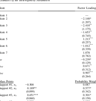
The possible correlation across disturbances in the indirect utility functions (the ei’s) can cause bias to the estimated coefficients. Such a correlation is likely because alternatives are defined by cross-classifying the discrete outcomes available to a sin-gle mother. For example, if a mother has strong preferences for work, these prefer-ences will appear in the error terms of all the choices in which she is employed (Alternatives 2–7). Similarly, if a mother possesses unobserved preferences for part-time (or full-time) work, this effect will appear in all the alternatives in which she is employed part-time (or full-time). Furthermore, mothers who receive childcare subsidies are a self-selected sample of the population. A mother’s decision about re-ceiving a childcare subsidy is likely to be correlated with her decision on labor sup-ply. For example, if a mother has strong preferences for work, she also may have a higher motivation to seek a childcare subsidy. Alternatively, the least employable mothers may be singled out for subsidies by administrators of the subsidy system (Blau and Tekin forthcoming). However, in a multinomial logit model, the correlation among the disturbance terms is restricted to zero because of the independence of ir-relevant alternatives assumption. A second source of error correlation is between the discrete outcomes and the continuous wage and childcare price equations. For exam-ple, a mother who is strongly motivated to work may also face better wage prospects. To deal with these correlations in a tractable way, the econometric model uses a random effects estimator with discrete factor approximations. This method obviates the need to evaluate multivariate integrals by approximating the distribution of the heterogeneity with a step function and ‘‘integrates out’’ through a weighted sum of probabilities (Blau and Hagy 1998; Picone et al. 2003; Mocan and Tekin 2003). Mroz (1999) shows that this estimator provides more robust estimates compared to methods imposing a specific distributional assumption.13
To implement this method, the following error structure is imposed on the distur-bances of the multinomial logit model and the continuous wage and childcare price equations:
ei=ui+rih; ð9Þ
jP=mP+rPh; ð10Þ
jPT=mPT+rPTh; ð11Þ
jFT=mFT+rFTh; ð12Þ
structure places the restriction that all the correlation among the error terms enters the model through the common factorhthat is assumed to have a discrete distribu-tion (Heckman and Singer 1984). In order to account for the missing price of child-care for mothers who do not pay for childchild-care and for the missing wage rate for mothers who are not employed, the Gaussian Quadrature is used. As described in Appendix 2, this is a convenient method to approximate normal integrals accurately at a low computing cost (Butler and Moffitt 1982).
The multinomial logit model and the equations for the price of childcare and two wage rates are estimated jointly with full information maximum likelihood, account-ing for nonindependence of errors across outcomes. The u’s in Equation 9 are as-sumed to have mean zero and to be independently extreme-value distributed and them’s in Equations 10–12 are assumed to have mean zero and to be independently normally distributed. The likelihood function and the details of the heterogeneity dis-tribution are discussed in Appendix 2.
IV. Data
The data are drawn from the 1997 National Survey of America’s Families (NSAF), which was conducted by the Urban Institute. The NSAF is repre-sentative of the United Stated civilian, noninstitutionalized population younger than 65. Residents of 13 states and households with income below 200 percent of the fed-eral poverty line are oversampled.14The full NSAF sample contains 44,461 house-holds. The NSAF is particularly well-suited for the purposes of this study for several reasons. First, it was specifically designed to collect detailed information on income, childcare, and participation in various programs, and to provide better data on such variables than can be obtained from most other surveys. Second, it was conducted after the enactment of the welfare reform legislation and many other important policy changes of early and mid-1990s. Third, the NSAF is one of the few national house-hold surveys with information on childcare subsidies.15Finally, it provides a rela-tively large sample of single mothers, who are the target group of welfare reform.
The main variables of interest are employment, childcare payment, and childcare subsidy receipt. In the NSAF, mothers are asked whether they receive any assistance paying for childcare, including help from a welfare or social services agency, an em-ployer, and a noncustodial parent. Mothers who report receiving assistance from a welfare or social services agency are coded as receiving a childcare subsidy.16 14. The 13 targeted states were Alabama, California, Colorado, Florida, Massachusetts, Michigan, Minne-sota, Mississippi, New Jersey, New York, Texas, Washington, and Wisconsin. These states contain more than half of the U.S. population and the welfare caseload. There are observations only from 29 states in the analyses sample and about 90 percent (3,653 individuals) of the sample lives in the oversampled states. 15. To my knowledge, the only other national survey with information on childcare subsidy receipt is the Kindergarten cohort of the Early Childhood Longitudinal Survey (ECLS-K).
Employment is specified as a trichotomous variable defined at zero hours of work, part-time work, and full-time work.17Childcare payment status is a binary variable equal to one if the mother reported any payment for childcare, and zero otherwise. The mother’s wage rate is computed as the ratio of her annual earnings to annual hours of work. In the NSAF, the childcare hours are collected for up to two randomly chosen children, one between ages 0–5 and the other between ages 6–12. These chil-dren are referred to as focal child I and focal child II in the NSAF. Childcare expen-ditures on the other hand, are collected for all children ages 0–12.18Therefore, the hourly childcare expenditure per child can be approximated by dividing the total childcare expenditures for all children ages 0–12 by the total childcare hours for all children ages 0–12. The later can be obtained by the sum of childcare hours for all children ages 0–5 (the product of the childcare hours for focal child I and the number of children ages 0–5) and childcare hours for all children ages 6–12 (the product of the childcare hours for focal child II and the number of children ages 6–12). However, the NSAF provides information only on the number of children ages 0–5 and ages 6–17. The number of children ages 6–12 can be obtained perfectly for those mothers with a focal child II and only one child ages 6–17 because that child has to be the only one the mother has ages 6–12. There is also no problem for mothers who do not have a focal child II because in this case the mother has no children ages 6–12 anyway. For mothers with a focal child II and with at least two children ages 6–17, I obtained the proportion of the U.S. population between ages 6 and 12 as a fraction of the total population ages 6 and 17 in 1997 from the U.S. Census Bureau. Then, this figure is multiplied by the total number of children ages 6–17 in the NSAF. Note that only 28 percent of the single mothers in the sample have more than one child between ages 6–12. However, estimation of the models ex-cluding these mothers with multiple children between ages 6 and 12 did not change the implications of the current results in a significant way.
According to the statute for federal eligibility for a childcare subsidy, ‘‘all eligible children must be younger than 13 and reside with a family whose income does not exceed 85 percent of the state median income for a family of the same size and whose parent(s) are working or attending a job training or educational program or who receive or need to receive protective services.’’ (U.S. Department of Health and Human Services 2000). The federal law allows states to set the eligibility criteria up to 85 percent of State Median Income, but in 1997, only nine states set income eligibility at the 85 percent level and seven states set it at less than 50 percent level. Data on state annual median income, income-eligibility rules, and the reimbursement rates are obtained from the Childcare Bureau’s Report of State Plans of the Child Care Development Block Grant (U.S. Department of Health and Human Services 2000). Because the sample includes only single mothers with at least a child younger than 13, every mother meets the first major eligibility criterion. States’ reimburse-ment rates vary by the age of the child and they are set on hourly, daily, weekly,
17. Mothers with weekly work hours from 1 to 35 are classified as working part-time and those with 35 and over are classified as working full-time. Similar definitions have previously been used in the childcare literature (Michalapoulos and Robins 2000).
or monthly bases. All figures are converted to an hourly base assuming full time care. Reimbursement rates sometimes vary within states. In these cases, the geographic re-gion that includes the largest city in the state is used.19
The other variables used in the multinomial choice model include the mother’s age, nonwage income, race, ethnicity, and binary indicators for the mother’s educa-tional attainment, health status, the presence of children by age, and the region of residence. These variables are included in the model to control for mother’s prefer-ences and her quality of childcare. Nonwage income is the sum of household income from nonmarket sources, excluding income from means-tested programs. The num-ber of family memnum-bers age 25 and over who live in the household are included to control for the availability of free care by a relative to the mother. Finally, the state unemployment rate for females is included in order to control for labor demand con-ditions that would affect preferences.
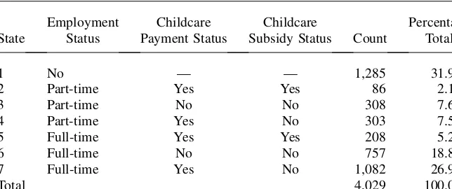
The empirical analysis is performed on a subsample of households headed by a single mother with at least one child younger than 13. The total sample includes 4,029 households. Table 2 displays the distribution of employment, childcare pay-ment, and childcare subsidy outcomes. About 68 percent of the single mothers in the sample are employed. The percentage of part-time and full-time working mothers is about 17 and 51, respectively. About 56 percent of part-time working mothers and
Table 2
Frequency Distributions of the Discrete Outcomes
State
Employment Status
Childcare Payment Status
Childcare
Subsidy Status Count
Percentage Total
1 No — — 1,285 31.9
2 Part-time Yes Yes 86 2.1
3 Part-time No No 308 7.6
4 Part-time Yes No 303 7.5
5 Full-time Yes Yes 208 5.2
6 Full-time No No 757 18.8
7 Full-time Yes No 1,082 26.9
Total 4,029 100.0
Source: 1997 National Survey of America’s Families.
63 percent of full-time working single mothers pay for childcare. The proportion of the sample receiving a childcare subsidy is about 12 percent among part-time work-ers and about 10 percent among full-time workwork-ers. Sixty-four percent of working mothers (1,756 mothers) in the sample are eligible for a childcare subsidy under the income eligibility rules set by states in 1997. Therefore, about 17 percent (294 mothers) of these eligible receive a childcare subsidy. Note that this number is close to the figure from a report by the Administration for Children and Families (1999), which estimates that 12–15 percent of eligible families received a CCDF subsidy in 1998–99. Definitions and the summary statistics are presented in Table 3. Employed mothers have a higher level of education than nonemployed mothers and full-time working mothers have a higher level of education than part-time working mothers. Whites have a higher rate of employment than both blacks and other races. Expect-edly, mothers working full-time earn higher wages on average compared to those working part-time.
V. Results
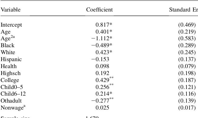
The results from the estimations of the childcare price and the full-time and part-full-time wage equations are presented in Appendix Tables A2 and A3. While space limitation precludes a detailed discussion of these results in the text, they are consistent with those usually found in the relevant literature. The results of the discrete choice model are presented in Table 4.20The reference category is alternative 1 in which the single mother does not work, does not pay for childcare, and does not receive a childcare subsidy. A likelihood ratio test rejected a model with a single price coefficient against a model that allowed price coefficients to vary by part-time and full-time employment status. Consistent with the predictions of the theoretical model, a higher price of childcare reduces the utility in alternatives in which the mother works and pays for childcare. The coefficient estimates suggest that a higher price of childcare is a stronger deterrent to full-time employment than it is to part-time employment. The estimated childcare price coefficients for full-time and part-time working mothers are 20.192 and20.093, respectively. The implied childcare price elasticities with respect to full-time and part-time employment are 20.139 and 20.068, respectively. The finding that the price elasticity with respect to part-time employment is smaller than that of full-time employment in absolute value is consistent with other studies that distinguish between part-time and full-time employment. For example, Powell (1998) estimates the elasticity to be –0.20 for part-time employment and –0.71 for full-time employment using a sample of married mothers from Canada; Connelly and Kimmel (2003b) find the elasticities to be
20.40 and –1.29 for part-time and for full-time employment, respectively, for a sam-ple of single mothers; and Michalopoulos and Robins (2000) estimate the elasticities to be 0.159 for part-time and20.342 for full-time using a sample of two-parent fam-ilies from Canada and the United States.
The price elasticity with respect to overall employment is calculated to be –0.121. This figure falls in the lower end of the range of estimates reported in the literature. However, it is particularly close to those from several studies that are similar to the current paper in terms of their use of a multinomial choice model in the estimation. Examples include20.09 of Ribar (1995) and20.38 of Blau and Robins (1988) who estimate a discrete choice model with multinomial logit;20.156 of Michalopoulos and Robins (2000) who estimate a multinomial logit distinguishing between full-time and part-time employment; and20.20 of Blau and Hagy (1998) who estimate a dis-crete choice model by a random effects estimator similar to the one employed in the present study.21Given that studies using similar estimation methods find small elas-ticities suggests that the true elasticity of employment may be small.
A comparison of the elasticity of employment found here to those from other stud-ies using samples of single mothers suggests that the elasticity found in this paper is smaller than most others reported in those studies. However, the figure found here is still not completely out of line with the literature, especially given the wide variation in the estimated elasticities in previous studies.22The overall price elasticity of pay-ing for care with respect to the price of childcare is20.148, which is also compara-ble to estimates in several other studies. For example, Blau and Hagy (1998) find an elasticity of20.34 for a sample of both married and single mothers, and Michalo-poulos, Robins, and Garfinkel (1992) estimate it to be20.298 for single mothers.
Turning to the wage effects, a higher part-time (full-time) wage increases the util-ity in those alternatives in which the mother works part-time (full-time), which is consistent with the predictions of the theoretical model. A likelihood ratio test rejected the model that restricted the part-time and full-time wage coefficients to be the same between the two employment types against a model that allowed sepa-rate effects. The coefficient estimates on the part-time and full-time wage sepa-rates are 0.217 and 0.995, respectively. The implied elasticity of full-time employment is 0.874 with respect to the full-time wage rate, and is20.090 with respect to the part-time wage rate. Similarly, the implied elasticity of part-time employment is 0.431 with respect to the part-time wage rate, and is20.097 with respect to the full-time wage rate. Combining the effects on the full-time and part-time employ-ment, the implied elasticity of overall employment is calculated to be 0.663 with respect to the full-time wage rate and 0.081 with respect to the part-time wage rate. These results indicate that the full-time wage is a much stronger determinant of
21. Note that Blau and Hagy (1998) use provider fee-based price measures in their analyses. When they repeated their analyses using consumer expenditure data, they found an elasticity of -0.06. The largest elas-ticity among these studies is Blau and Robins (1988). However, the authors included the price of childcare in all of the outcomes in which the mother was employed instead of only those in which she used paid care. Therefore, the comparison would be more meaningful among the other studies, and this would further re-inforce the proposition that the actual elasticity may be small.
Table 3
Variable Definitions and Descriptive Statistics
Variable Definition
Full
Sample Nonemployed
Employed Part-Time
Employed Full-Time
Age = Mother’s age in years 31.936 30.565 31.548 32.929
(6.892) (6.901) (6.868) (6.734)
Black = 1 if mother is black, = 0 otherwise 0.322 0.356 0.288 0.312
(0.467) (0.479) (0.453) (0.463)
White = 1 if mother is white, = 0 otherwise 0.648 0.607 0.684 0.662
(0.478) (0.489) (0.465) (0.473)
Othracea = 1 if mother is of other race, = 0 otherwise 0.030 0.037 0.027 0.026
(0.169) (0.188) (0.163) (0.159)
Northeast = 1 if mother resides in Northeast, = 0 otherwise 0.228 0.275 0.254 0.191
(0.420) (0.447) (0.436) (0.393)
Midwest = 1 if mother resides in Midwest, = 0 otherwise 0.294 0.224 0.331 0.325
(0.456) (0.417) (0.471) (0.468)
South = 1 if mother resides in South, = 0 otherwise 0.310 0.316 0.245 0.329
(0.463) (0.465) (0.431) (0.470)
Westa = 1 if mother resides in West, = 0 otherwise 0.167 0.185 0.169 0.155
(0.373) (0.389) (0.375) (0.362)
Health = 1 if mother is in good or better health, = 0 otherwise 0.932 0.903 0.947 0.946
(0.251) (0.296) (0.224) (0.227)
Nodegreea = 1 if mother has less than high-school degree 0.156 0.292 0.116 0.084
(0.363) (0.455) (0.321) (0.277)
Highsch = 1 if mother has high-school or some college degree, = 0 otherwise
0.732 0.644 0.769 0.774
(0.443) (0.479) (0.422) (0.418)
The
Journal
of
Human
Hispanic = 1 if mother is of Hispanic ethnicity, = 0 otherwise 0.143 0.202 0.123 0.112
(0.350) (0.401) (0.329) (0.316)
Othadult = Number of family members aged 25
or higher living in the household
0.353 0.382 0.318 0.346
(0.691) (0.728) (0.667) (0.638)
Nonwage (/1000) = Annual nonwage income 4.558 3.444 4.390 5.314
(7.538) (6.94) (6.885) (7.304)
Child 0–6 = 1 if mother has a child age 0–5 only, = 0 otherwise 0.331 0.380 0.334 0.299
(0.471) (0.486) (0.472) (0.458)
Child 6–12 = 1 if mother has a child age 6–12 only, = 0 otherwise 0.446 0.333 0.445 0.516
(0.497) (0.471) (0.497) (0.500)
Childbotha = 1 if mother has children in both age Groups 0–5 and 6–12, = 0 otherwise
0.224 0.287 0.221 0.185
(0.417) (0.453) (0.415) (0.388)
Sunempb = State’s unemployment rate for females in 1997 5.181 5.362 5.085 5.101
(1.448) (1.424) (1.476) (1.464)
Wagepart-time = Hourly rate of part-time wage — — 6.691 —
(1.459)
Wagefull-time = Hourly rate of full-time wage — — — 8.223
(3.412)
Pricechildcare = Hourly price of childcare — — 2.214 2.062
(1.810) (1.779)
4,029 1,285 697 2,047
Note: Standard deviations are in parentheses. a. Omitted category, b. Source: U.S. Census Bureau.
T
ekin
Table 4
Estimates of the Discrete Choice Model
Variable
State 2 Work=Part-Time
Paid Care=Yes Subsidy=Yes
State 3 Work=Part-Time
Paid Care=No Subsidy=No
State 4 Work=Part-Time
Paid Care=Yes Subsidy=No
State 5 Work=Full-Time
Paid Care=Yes Subsidy=Yes
State 6 Work=Full-Time
Paid Care=No Subsidy=No
State 7 Work=Full-Time
Paid Care=Yes Subsidy=No
Intercept 2.121*** 21.126* 20.672 20.703 21.224 0.921* (0.438) (0.622) (0.403) (0.552) (0.987) (0.524)
Age 20.125** 0.131* 20.097* 0.231 0.131 0.091**
(0.059) (0.068) (0.058) (0.151) (0.089) (0.038) Northeast 0.761* 0.689** 0.459** 0.412** 0.601* 0.452**
(0.427) (0.310) (0.212) (0.187) (0.353) (0.188) Midwest 0.339 0.744** 0.619** 0.939*** 1.181** 0.902**
(0.495) (0.371) (0.311) (0.436) (0.576) (0.405)
South 0.181 20.359 0.101 20.544* 20.697* 0.608
(0.302) (0.392) (0.389) (0.321) (0.411) (0.567)
Black 20.448 20.514 20.278 0.529 0.763 0.054
(0.359) (0.401) (0.267) (0.465) (0.654) (0.104)
White 0.632 0.395* 0.255* 0.904* 1.256* 0.514**
(0.558) (0.214) (0.142) (0.478) (0.735) (0.243) Hispanic 20.667* 20.491 20.250** 20.623 20.489 20.589*
(0.388) (0.687) (0.113) (0.573) (0.623) (0.334)
Health 20.399 20.144 0.038 20.332 0.102 0.341
(0.590) (0.219) (0.104) (0.367) (0.451) (0.387) Highsch 0.897*** 0.282** 0.801** 0.677** 1.289** 0.921**
(0.288) (0.141) (0.379) (0.322) (0.601) (0.452)
The
Journal
of
Human
Nonwage 20.768* 20.523** 20.203** 0.103 0.213 20.210** (0.402) (0.259) (0.101) (0.151) (0.322) (0.123)
Child 0-5 20.311 0.367 0.044 20.091 20.135 20.049
(0.444) (0.283) (0.059) (0.101) (0.348) (0.078) Child 6-12 0.367 0.344** 20.110 20.299 20.556 0.189
(0.359) (0.175) (0.077) (0.222) (0.499) (0.260) Othadult 0.068 0.204* 20.067 20.169 20.301 20.383* (0.103) (0.106) (0.099) (0.141) (0.314) (0.211) Sunemp 20.043 20.032 20.035 20.089* 20.104* 20.118* (0.049) (0.051) (0.028) (0.051) (0.055) (0.067) Pricechildcare 20.093 — 20.093 20.192** — 20.192**
(0.081) (0.081) (0.088) (0.088)
Log 0.217** 0.217** 0.217** — — —
Wagepart-time (0.097) (0.097) (0.097)
Log Wagefull-time — — — 0.995*** 0.995*** 0.995***
(0.314) (0.314) (0.314) Number of
observations
4,029
Log likelihood 210,569
Notes: Standard errors are in parentheses. The symbols *, **, and *** represent statistical significance at the 10 percent, 5 percent, and 1 percent levels, respectively. a. Variable is divided by 1,000.
T
ekin
overall employment than the part-time wage rate. They also suggest that there is an important difference in the nature of part-time and full-time employment types for single mothers. Although the previous studies do not distinguish between the two wage rates as done in this paper, these results are in line with the previous research which finds that wages have a larger effect on full-time employment than on part-time employment (Powell 1998, Connelly and Kimmel 2003b).
The effects of other explanatory variables are in most cases consistent with one’s expectations and with those found in the relevant literature For example, a higher nonwage income decreases the likelihood that a mother would choose an alternative in which she is employed. A higher level of education increases the likelihood that a mother would choose an alternative in which she is employed. Being white is asso-ciated with a higher likelihood of being employed than being black or other race.
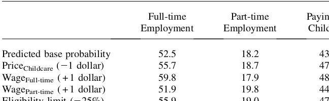
To examine the policy implications of the empirical results further, several simu-lations are generated. While these simusimu-lations do not refer to any particular policy proposal, they help illustrate the effectiveness of different policy options in increas-ing employment. In each simulation, a price of childcare and a part-time and a full-time wage rate are predicted for each mother in the sample by using the coefficient estimates. Then the probabilities for each alternative are computed for each mother, integrating over the heterogeneity distribution, which are then averaged over the sample. Simulation results are presented in Table 5. The first simulation reduces the hourly price of childcare by one dollar. This can be considered as a subsidy that is available to all working mothers and is equivalent to an annual subsidy of about 2,080 dollars for a full-time, full-year working mother who pays for childcare. Based on the coefficient estimates, a one-dollar reduction in the price of childcare would increase full-time employment by 3.2 percentage points (a 6.1 percent increase) and part-time employment by 0.5 percentage point (a 2.7 percent increase). Combin-ing these two effects, the overall employment would increase by 3.7 percentage points (a 5.2 percent increase) in response to a one-dollar subsidy. Finally, the prob-ability of paying for childcare would increase by 4 percentage points (9.3 percent) as a result of this subsidy.
When the full-time wage rate is hypothetically subsidized by one dollar per hour of work, the probability of full-time employment would increase by 7.3 percentage points (13.9 percent) and the probability of part-time employment would decrease by
Table 5
Simulations of Employment and Childcare Payment Probabilities
Full-time Employment
Part-time Employment
Paying for Childcare
Predicted base probability 52.5 18.2 43.2
PriceChildcare(21 dollar) 55.7 18.7 47.2
WageFull-time( + 1 dollar) 59.8 17.9 48.9
WagePart-time( + 1 dollar) 51.9 19.8 44.0
0.3 percentage point (1.6 percent). As a result of this subsidy, the overall employ-ment would increase by 7 percentage points (9.9 percent). Finally, a one-dollar per hour subsidy for the part-time wage rage would only generate a 1.6 percentage point (8.8 percent) increase in part-time employment and a 0.6 percentage point (1.1 per-cent) decrease in full-time employment, which represents a 1 percentage point (1.4 percent) increase in overall employment.
The full-time wage elasticity of paying for care is estimated to be 0.711 and the part-time wage elasticity of paying for care is estimated to be 0.108. Similar to the effect on employment, the full-time wage rate is a much stronger determinant of pay-ing for childcare than the part-time wage rate. As shown in Table 5, a one-dollar per hour subsidy for the full-time wage rate would lead to a 5.7 percentage point (13.2 percent) increase in using paid childcare. Finally, a one-dollar subsidy for part-time wage would generate a 0.8 percentage point (1.9 percent) increase in using paid care. While these simulations give some idea about the effectiveness of wage and childcare subsidies on increasing employment, they do not provide insights into the relative cost-effectiveness of these subsidies. That is, they do not answer the question: which type of subsidy would generate the largest additional number of hours of work per dollar spent by the government? Following Blau (2003), some insights can be gained about the cost-effectiveness of wage and childcare subsidies using the estimates obtained in this paper and making a few simplifying assumptions. In particular, assume that there are no general equilibrium effects of subsidies and that hours of work are not influenced by subsidies, that is, subsidies can induce indi-viduals to move from part-time work to full-time work or vice-versa, but within each type of work, the hours of work are not affected (offsetting income and substitution effects). Also assume that subsidies are additive for analytic convenience. As de-scribed in detail in Appendix 3, under these assumptions and for a wide range of plausible parameters, the additional hours of work per dollar of government expen-diture generated by a childcare subsidy (CES) would exceed those of wage subsidies (CEFTfor a full-time wage subsidy andCEPTfor a part-time wage subsidy). For ex-ample, a subsidy rate of 50 percent would yield aCESof 0.084, aCEFTof 0.072, and aCEPTof only 0.001. Although a wage subsidy would at first appear to be a more direct method to increase employment, a childcare subsidy would actually be more cost-effective. This is because a wage subsidy provides benefits to all working mothers while a childcare subsidy provides benefits only to those working mothers who use paid childcare (Blau 2003). Therefore, a childcare subsidy would usually generate more hours of work per dollar spent by the government, which would make it a more cost-effective policy tool.
The first row in Table 5 presents the distribution of the outcome probabilities from the empirical model. These figures indicate that the model performs well in terms of fitting the actual data. The estimated full-time employment and childcare payment probabilities come within 2–3 percentage points of the corresponding figures from the sample. As discussed earlier, one of the contributions of this paper is that it includes the childcare subsidy receipt as an additional alternative in the mother’s choice set and that the childcare price is adjusted for the amount of the subsidy in the empirical analyses. In order to test the sensitivity of the results to this and the assumptions made in the implementation, the system of equations is reestimated ex-cluding the subsidy decision from the choice set. In this case, a single mother only makes a decision for employment and childcare payment, which generates a model with five alternatives. The results show that the responses of employment and child-care payment to the price of childchild-care are more elastic in the five-choice model rel-ative to the results presented in this paper. The elasticity of overall employment with respect to the price of childcare is estimated to be –0.399 and the elasticity of paying for care is estimated to be –0.468. This may actually explain in part why the child-care price elasticity found in this paper is relatively lower than some of those in the literature, especially for single mothers.
Note that the amount of childcare expenditures in the survey is reported by the mother and this is assumed to represent the amount net of subsidy,Ps-Ss, for those who receive one. This is equivalent to assuming that all subsidies were directly paid to the provider and any expenditure made by the mother represents her out-of-pocket payment, not the total price of childcare. This assumption is necessary because it is not possible to identify in the NSAF what method the mother uses in paying for childcare. If this assumption is incorrect,Ps-Sswould be overestimated. If voucher versus direct payment to the provider were random and uncorrelated with the explan-atory variables in the model, then the childcare price coefficient would still be unbi-ased. If this is not the case, however, the price effect may be biunbi-ased. In order to test the sensitivity of the results to this assumption, I reestimated the equations treating the subsidy recipients as if the price of childcare for them were unobserved. This allowed me to avoid having to make an assumption as to whether the cost of child-care is subsidized with a voucher or through a direct payment to the provider. There-fore, the price of childcare is substituted with a regression function for these mothers, just like those who use unpaid childcare. Note that this implementation is necessary only for 294 mothers in the sample who reported receiving a subsidy. The price elas-ticity of overall employment is estimated to be –0.133 and the price elaselas-ticity of pay-ing for care is estimated to be20.174. These results are close enough to those of the benchmark model not to change any of the current implications in a meaningful way.
VI. Conclusions
childcare prices and wages on the behavior of single mothers. This paper examines the effects of the price of childcare and the wage rates on employment and childcare payment decisions of single mothers. It contributes to the literature in several dimen-sions. First, it uses data from a survey conducted after welfare reform and other important policy changes of early and mid-1990s. Second, the empirical analysis incorporates the childcare subsidy receipt into the mother’s choice set and allows for an adjustment for the price of childcare by the amount of subsidy for eligible mothers who receive one. Third, it distinguishes between the part-time and full-time employment sectors, as well as the wage rates associated with each of these sectors. The estimated elasticity of overall employment with respect to the price of child-care is20.12, which falls in the lower end of the range of estimates found in the literature. The elasticities of employment with respect to full-time and part-time wages are estimated to be 0.66 and 0.08, respectively. The results suggest that single mothers who are employed full-time are more sensitive to the changes in the price of childcare than those who are employed part-time. A lower price of childcare in-creases employment and the use of paid childcare among those who are employed full-time, but it has a much smaller impact on those who are employed part-time.
Similarly, full-time working mothers are found to be much more sensitive to wage changes than part-time working mothers. These findings point to the importance of distinguishing between the part-time and full-time work when analyzing the responses of single mothers to the price of childcare. One possible explanation for these find-ings is that income from part-time employment may not be rewarding enough to in-duce mothers to leave welfare and seek employment even with a reduction in the price of childcare. It is also possible that part-time working mothers may have more flexible work schedules and may be able to find alternative childcare arrangements easier than full-time working mothers. This may then reduce the degree of their sen-sitivity to the price of childcare.
One implication of the findings is that state policies that provide financial incen-tives to mothers are likely to have reasonably large effects on the work effort of sin-gle mothers if targeted to full-time employment. The effects of such policies would be much smaller if targeted to part-time employment. These findings are particularly meaningful as some of the current debate over the reauthorization of the 1996 wel-fare reform bill includes proposals that aim to increase not only the employment of low-income individuals but their hours of work as well. For example, the budget reconciliation bill that includes changes to TANF and childcare assistance imposes additional work requirements. Specifically, the bill includes a stipulation that requires 90 percent of the welfare families to participate in work activities for at least 35 hours per week (Parrott, Park, and Greenstein 2006).
An analysis of cost-effectiveness of wage and childcare and wage subsidies indi-cate that the cost-effectiveness, as measured by the additional numbers of hours of work generated per dollar of government expenditure, is usually higher for a child-care subsidy than a wage subsidy. This is likely to due to the fact that a wage subsidy provides benefits to all working mothers while a childcare subsidy provides benefits only to those working mothers who use paid childcare (Blau 2003).
Robins 2000; Blau and Robins 1988). This similarity is important because one of the puzzling questions that remain unanswered in the childcare literature is the uncer-tainty in the size of the elasticity of employment with respect to the price of child-care. The small elasticity found in these papers, along with the current paper, contributes to resolving this issue. However, given that none of these papers other than the current one uses a sample of single mothers, caution must still be exercised in making a generalization. An avenue for future research would be to estimate mod-els with different data sets focusing on samples of single mothers.
Appendix 1
The Choice Set
It is assumed that a single mother makes her decision among the choices of no em-ployment, part-time emem-ployment, and full-time employment. Total household in-come in these employment states can be expressed as
INðIncome when not employedÞ=N;
IPTðIncome when employed part-timeÞ=N+WPTH;and
IFTðIncome when employed full-timeÞ=N+WFTH;
whereNis the nonwage income. There are three scenarios to consider:
1. The mother may be ineligible for a childcare subsidy regardless of her work hours (IN>E, whereEdenotes the income eligibility limit for a childcare sub-sidy). Alternatively, the household income may satisfy the eligibility condition when not employed (IN<E), but she may be ineligible when employed part-time or full-time (IPT>E). In these cases, subsidy receipt is not part of the mother’s choice set and she will make a decision among the alternatives 1, 3, 4, 6, and 7 listed in Table A1. In Alternative 1, she is not employed and is therefore ineligible for a subsidy. In Alternatives 3 and 6, no paid childcare is used, thus no subsidy can be received. In Alternatives 4 and 7, the mother is employed and pays for childcare, but is ineligible for a childcare subsidy since her income exceeds the eligibility limit.
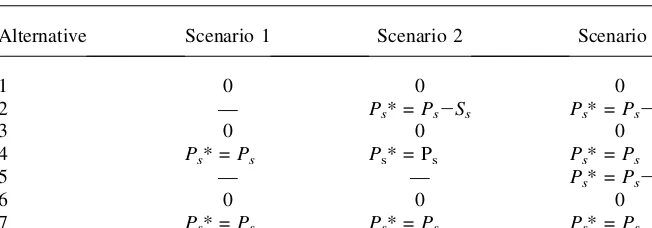
full-time, it will also satisfy this condition when she is employed part-time. Therefore, all seven states listed in Table A1 are in the mother’s choice set. The price of childcare that a mother faces is alternative-specific. If Alternatives 2 or 5 are in the mother’s choice set, the price of childcare in these alternatives is net of the subsidy amount. The appropriate price of childcare under each scenario is dis-played in Table A1. ThePsis the market price of childcare andPs* is the price that the mother faces when making her decisions. If the mother is observed in Alterna-tives 4 or 7, that is, she pays for childcare but does not use a subsidy, then the ob-served price is the market price of childcare, Ps, and therefore the price net of subsidy isPs-Ss. Of course, the use ofPs-Ssis necessary only if the mother is eligible for a subsidy as explained above. If the mother is observed in Alternatives 2 or 5, that is, she uses paid care and receives a childcare subsidy, then the observed price is the market price net of subsidy,Ps-Ss. This is because this figure comes from the mother’s report on her childcare expenditures. As explained in the paper, it is as-sumed that mother reports her childcare expenditures net of subsidy if she receives one. Then the market price for Alternatives 4 and 7, in which paid childcare is used without a subsidy, can be obtained by addingSsto thePs-Ss.23If the mother is in Alternatives 3 or 6, in which she does not pay for childcare, or in Alternative 1, in which she is not employed, a childcare price is still needed to be used in the like-lihood function. In this case, the market price of childcare is accounted for using the Gaussian Quadrature explained in Appendix 2. Finally, the market price net of subsidy is calculated by subtracting theSsfrom the estimated market price in the sub-sidy Alternatives 2 and 5 if the mother is eligible for a subsub-sidy. This is necessary to express the likelihood function correctly.
Table A1
The Relevant Price of Childcare under Different Scenarios
Alternative Scenario 1 Scenario 2 Scenario 3
1 0 0 0
2 — Ps* =Ps2Ss Ps* =Ps2Ss
3 0 0 0
4 Ps* =Ps Ps* = Ps Ps* =Ps
5 — — Ps* =Ps2Ss
6 0 0 0
7 Ps* =Ps Ps* =Ps Ps* =Ps
Appendix 2
A. Heterogeneity Specification
Assume that theuin Equation 9 is drawn from independent extreme-value distribu-tions, and thems in Equations 10–12 are drawn from independent mean-zero normal distributions. Further, the distribution ofhin Equations 9–12 is assumed to be given by the following step function:
Probðh=nmÞ=pm; m = 1;...;M; pm $0; and
+ M
m= 1 pm= 1;
wherenmis themthpoint of support in the factor distribution, andpmis the proba-bility that the factor m takes on the valuenm. Mis the number of points in the support of the distribution ofh. Theps,r, andns are parameters to be estimated along with other coefficients of the explanatory variables in the model.
Following Blau and Hagy (1998), thens andps are parameterized as follows:
n1=20:5; nm=
expðqmÞ 1 + expðqmÞ20:5
ðm= 2;...;M21Þ; and nM= 0:5;
and
pm= expðrmÞ 1 + +
M21
m= 1 expðrmÞ
m= 1;.;M21; and pM= 1
1 + + M21
m= 1 expðrmÞ
;
whereqmandrmare free parameters to be estimated.
B. The Likelihood Function
Note that the total number of alternatives relevant to each mother depends on her eligibility for a childcare subsidy at different employment types. Aside from her el-igibility, a single mother’s contribution to the likelihood function depends on her employment and childcare payment status as well. There are five possible cases available to each mother. These cases are considered below:
In Case 1, the mother is employed full-time and pays for childcare. Then, we ob-serve the full-time wage rate and the price of childcare, but do not obob-serve the part-time wage rate. LetDi= 1 if the motherjchooses statei, andDi= 0 otherwise. Then the likelihood function contribution for this mother is
Lj= + M
m= 1
pmPrjðDijhm;Ps*;lnWFTÞPrjðPsjhmÞPrjðlnWFTjhmÞ; ð13Þ
wage rate. Prj(Psj hm) is the probability of observing Ps conditional on hm, and Prj(lnWFTjhm) is the probability of observing lnWFT conditional onhm.
In Case 2, the mother is employed part-time and pays for childcare. Therefore, we observe the part-time wage rate and price of childcare, but not the full-time wage rate. The likelihood function contribution for this mother is
Lj= + M
m= 1
pmPrjðDijhm;Ps*;lnWPTÞPrjðPsjhmÞPrjðlnWPTjhmÞ:
ð14Þ
In Case 3, the mother is employed full-time and does not pay for childcare. There-fore, we observe the full-time wage rate, but not the part-time wage rate and price of childcare. The likelihood function contribution for this mother is
Lj= + M
m= 1
pmPrjðDijhm;lnWFTÞPrjðlnWFTjhmÞ ð15Þ
Table A2
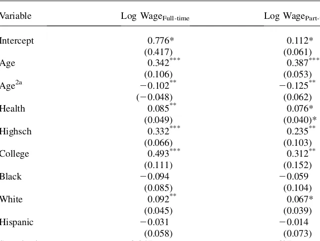
Estimates from the Wage Models
Variable Log WageFull-time Log WagePart-time
Intercept 0.776* 0.112*
(0.417) (0.061)
Age 0.342*** 0.387***
(0.106) (0.053)
Age2a 20.102** 20.125**
(20.048) (0.062)
Health 0.085** 0.076*
(0.049) (0.040)*
Highsch 0.332*** 0.235**
(0.066) (0.103)
College 0.493*** 0.312**
(0.111) (0.152)
Black 20.094 20.059
(0.085) (0.104)
White 0.092** 0.067*
(0.045) (0.039)
Hispanic 20.031 20.014
(0.058) (0.073)
Sample size 2,047 697
Notes: Standard errors are in parentheses. The model also includes state fixed effects.
The symbols *, **, and *** represent statistical significance at the 10 percent, 5 percent, and 1 percent levels, respectively.
In Case 4, the mother is employed part-time and does not pay for childcare. There-fore, we observe the part-time wage rate, but not the full-time wage rate and price of childcare. The likelihood function contribution for this mother is
Lj= + M
m= 1
pmPrjðDijhm;lnWPTÞPrjðlnWPTjhmÞ: ð16Þ
Finally, in Case 5, the mother is not employed and does not pay for childcare. Therefore, we do not observe the full-time wage rate, the part-time wage rate, and the price of childcare. The likelihood function contribution for this mother is
Lj= + M
m= 1
pmPrjðDijhmÞ: ð17Þ
Below, the exact form of the likelihood function contributions for Cases 1 and 5 are derived. The basic approach for other cases is similar and the exact forms are available from the author.
The likelihood function contribution for a mother in Case 1 can be rewritten as
Lj=
where Prj(Di j hm, Ps*, lnWFT, lnWPT) represents the probability that mother j chooses state i conditional on the values of h,Ps*, lnWFT, and lnWPT. Prj(Psjhm), Prj(lnWFT j hm), and Prj(lnWPTjhm) are the probabilities of observing Ps, lnWFT, and lnWPT conditional onhm. As described in the paper, the regression functions for lnWFT, and lnWPTare specified as follows:
lnWPTj=Dsd1PT+Xjd2PT+mPT+rPThm; ð19Þ
lnWFTj=Dsd1FT+Xjd2FT+mFT+rFThm: ð20Þ
Given the assumptions on the distributions of error terms in Equations 9–12, Equa-tion 18 can be rewritten as
Lj=
withb1[0, andKis total number of alternatives available to the mother and can take on the values of five, six, or seven, depending on the eligibility of mother j
for a childcare subsidy as discussed in Appendix 1.
Equation 21 integrates out the distribution ofhmthrough a weighted sum of prob-abilities using the random effects estimator as discussed in the paper. To integrate out the distribution of the error term of lnWPT, the Gaussian Quadrature method is used.24 The Gaussian Quadrature approximates an integral of the form,R
exp(-r2)h(r)dr, as +tY
wth(rt), whereYis the number of points used in the approximation,wtis the weight applied to thetth point of support, andrtis thetth point of support in the approximation.wtandrtare available in statistical handbooks for alternative values ofY.
Note that Equation 21 has the formR
exp(-r2)h(r)dr, wherer=mPT/(sPTO2), and
Incorporating the Gaussian Qudrature into Equation 21, the likelihood function contribution of motherjcan be approximated as follows:
Lj+t
Under similar distributional assumptions about us andms,Ljcan be rewritten as follows:
Equation 23 integrates over the error distributions of the price of childcare, the full-time, and the part-time wage. This equation is similar to Case 1 in which the in-tegration was necessary only for the distribution of the error term in the lnWPT equation. Also, note that each of the integral terms in Equation 23 can be