Calculus
for Biology and Medicine
Calculus
for Biology and Medicine
Claudia Neuhauser
University of Minnesota
Prentice Hall
Senior Project Editor:Joanne Dill Editorial Assistant:Joanne Wendelken Senior Managing Editor:Karen Wernholm Senior Production Supervisor:Tracy Patruno
Project Managers:Rob Merenoff and Lifland et al., Bookmakers Manufacturing Buyer:Debbie Rossi
Executive Marketing Manager:Jeff Weidenaar Marketing Assistant:Kendra Bassi
Art Director:Heather Scott AV Project Manager:Tom Benfatti
Manager, Cover Visual Research & Permissions:Elaine Soares Cover/Interior Designer:Tamara Newnam
Compositor:Dennis Kletzing
Art Studio:Laserwords Private Limited
Cover Image:HI Virus infecting cell / Shutterstock
Photo credits appear on page C1 and constitute a continuation of the copyright page.
Many of the designations used by manufacturers and sellers to distinguish their products are claimed as trademarks. Where those designations appear in this book, and Pearson was aware of a trademark claim, the designations have been printed in initial caps or all caps.
Library of Congress Cataloging-in-Publication Data Neuhauser, Claudia, 1962–
Calculus for biology and medicine / Claudia Neuhauser.--3rd ed.
p. cm.
Includes bibliographical references and index.
ISBN 978-0-321-64468-8 (alk. paper)
1. Biomathematics--Textbooks. 2. Medicine--Mathematics Textbooks.
I. Title.
QH323.5.N46 2011 515--dc22
2011027223
Copyright © 2011, 2004, 2000 Pearson Education, Inc. All rights reserved. No part of this publication may be reproduced, stored in a retrieval system, or transmitted, in any form or by any means, electronic, mechanical, photocopying, recording, or otherwise, without the prior written permission of the publisher. Printed in the United States of America. For information on obtaining permission for use of material in this work, please submit a written request to Pearson Education, Inc., Rights and Contracts Department, 501 Boylston Street, Suite 900, Boston, MA 02116, fax your request to 617-671-3447, or e-mail at http://www.pearsoned.com/legal/permissions.htm.
1 2 3 4 5 6 7 8 9 10—EB—13 12 11 10 09
ISBN 10: 0-321-64468-9 ISBN 13: 978-0-321-64468-8
About the Author
Claudia Neuhauser
is Vice Chancellor for Academic Affairs and Director of the Center for Learning Innovation at the University of Minnesota Rochester (UMR). She is a Distinguished McKnight University Professor, Howard Hughes Medical Institute Professor, and Morse-Alumni Distinguished Teaching Professor. She received her Diploma in Mathematics from the Universität Heidelberg (Germany), and a Ph.D. in Mathematics from Cornell University. Before joining UMR in July 2008, she was Professor and Head in the Department of Ecology, Evolution and Behavior at the University of Minnesota Twin Cities, and a faculty member in mathematics departments at the University of Southern California, UW-Madison, University of Minnesota, and UC Davis.Dr. Neuhauser’s research is at the interface of ecology and evolution. She investigates effects of spatial structure on community dynamics, in particular, the effect of competition on the spatial structure of competitors and the effect of symbionts on the spatial distribution of their hosts. In addition, her research in population genetics has resulted in the development of statistical tools for random samples of genes.
In her role as Director of the Center for Learning Innovation at the University of Minnesota Rochester, Dr. Neuhauser is responsible for the development of the Bachelor of Science in Health Sciences. The Center promotes a learner-centered, concept-based learning environment in which ongoing assessment guides and monitors student learning and is the basis for data-driven research on learning. Dr. Neuhauser’s interest in furthering the quantitative training of biology undergraduate students has resulted in a textbook titledCalculus for Biology and Medicineand a web page called Numb3r5 Count! (http://bioquest.org/numberscount/). In her spare time, she enjoys riding her bike, working out in the gym, and reading history and philosophy.
Contents
Preface xi
1 Preview and Review 1
1.1 Preliminaries 2
1.1.1 The Real Numbers 2 1.1.2 Lines in the Plane 4 1.1.3 Equation of the Circle 6 1.1.4 Trigonometry 7
1.1.5 Exponentials and Logarithms 8 1.1.6 Complex Numbers and Quadratic
Equations 11
1.2 Elementary Functions 16 1.2.1 What Is a Function? 16 1.2.2 Polynomial Functions 19 1.2.3 Rational Functions 21 1.2.4 Power Functions 23 1.2.5 Exponential Functions 24 1.2.6 Inverse Functions 28 1.2.7 Logarithmic Functions 30 1.2.8 Trigonometric Functions 32
1.3 Graphing 39
1.3.1 Graphing and Basic Transformations of Functions 39
1.3.2 The Logarithmic Scale 42
1.3.3 Transformations into Linear Functions 43 1.3.4 From a Verbal Description to a Graph
(Optional) 50 Key Terms 58 Review Problems 58
2 Discrete Time Models, Sequences, and Difference Equations 62
2.1 Exponential Growth and Decay 62 2.1.1 Modeling Population Growth in Discrete
Time 62 2.1.2 Recursions 65
2.2 Sequences 68
2.2.1 What Are Sequences? 68 2.2.2 Limits 71
2.2.3 Recursions 75
2.3 More Population Models 79
2.3.1 Restricted Population Growth: The Beverton–Holt Recruitment Curve 80 2.3.2 The Discrete Logistic Equation 82 2.3.3 Ricker’s Curve 85
2.3.4 Fibonacci Sequences 86 Key Terms 89
Review Problems 89
3 Limits and Continuity 91
3.1 Limits 91
3.1.1 An Informal Discussion of Limits 92 3.1.2 Limit Laws 97
3.2 Continuity 102
3.2.1 What Is Continuity? 102 3.2.2 Combinations of Continuous
Functions 105
3.3 Limits at Infinity 109
3.4 The Sandwich Theorem and Some Trigonometric Limits 113
3.5 Properties of Continuous Functions 119
3.5.1 The Intermediate-Value Theorem 119 3.5.2 A Final Remark on Continuous
Functions 122
3.6 A Formal Definition of Limits (Optional) 123
Key Terms 129 Review Problems 129
4 Differentiation 132
4.1 Formal Definition of the Derivative 133
4.1.1 Geometric Interpretation and Using the Definition 135
4.1.2 The Derivative as an Instantaneous Rate of Change: A First Look at Differential Equations 138
4.1.3 Differentiability and Continuity 141
4.2 The Power Rule, the Basic Rules of Differentiation, and the Derivatives of Polynomials 145
4.3 The Product and Quotient Rules, and the Derivatives of Rational and Power Functions 151
4.3.1 The Product Rule 151 4.3.2 The Quotient Rule 154
4.4 The Chain Rule and Higher Derivatives 159
4.4.1 The Chain Rule 159
4.4.2 Implicit Functions and Implicit Differentiation 165
4.4.3 Related Rates 167 4.4.4 Higher Derivatives 169
4.5 Derivatives of Trigonometric Functions 174
vii
4.6 Derivatives of Exponential Functions 178
4.7 Derivatives of Inverse Functions, Logarithmic Functions, and the Inverse Tangent Function 183
4.7.1 Derivatives of Inverse Functions 183 4.7.2 The Derivative of the Logarithmic
Function 188
4.7.3 Logarithmic Differentiation 190
4.8 Linear Approximation and Error Propagation 193
Key Terms 200 Review Problems 200
5 Applications of Differentiation 202
5.1 Extrema and the Mean-Value Theorem 202
5.1.1 The Extreme-Value Theorem 202 5.1.2 Local Extrema 204
5.1.3 The Mean-Value Theorem 208
5.2 Monotonicity and Concavity 215 5.2.1 Monotonicity 216
5.2.2 Concavity 218
5.3 Extrema, Inflection Points, and Graphing 224
5.3.1 Extrema 224 5.3.2 Inflection Points 230
5.3.3 Graphing and Asymptotes 231
5.4 Optimization 237 5.5 L’Hospital’s Rule 245
5.6 Difference Equations: Stability (Optional) 253
5.6.1 Exponential Growth 254 5.6.2 Stability: General Case 255 5.6.3 Examples 258
5.7 Numerical Methods: The Newton–Raphson Method (Optional) 262
5.8 Antiderivatives 267 Key Terms 273 Review Problems 273
6 Integration 276
6.1 The Definite Integral 276 6.1.1 The Area Problem 277 6.1.2 Riemann Integrals 280
6.1.3 Properties of the Riemann Integral 286
6.2 The Fundamental Theorem of Calculus 293
6.2.1 The Fundamental Theorem of Calculus (Part I) 294
6.2.2 Antiderivatives and Indefinite Integrals 298
6.2.3 The Fundamental Theorem of Calculus (Part II) 301
6.3 Applications of Integration 306
6.3.1 Areas 307
6.3.2 Cumulative Change 311 6.3.3 Average Values 312
6.3.4 The Volume of a Solid (Optional) 315 6.3.5 Rectification of Curves (Optional) 318 Key Terms 323
Review Problems 323
7 Integration Techniques and Computational Methods 325
7.1 The Substitution Rule 325
7.1.1 Indefinite Integrals 325 7.1.2 Definite Integrals 329
7.2 Integration by Parts and Practicing Integration 334
7.2.1 Integration by Parts 334 7.2.2 Practicing Integration 340
7.3 Rational Functions and Partial Fractions 344
7.3.1 Proper Rational Functions 344 7.3.2 Partial-Fraction Decomposition 345
7.4 Improper Integrals 351
7.4.1 Type 1: Unbounded Intervals 351 7.4.2 Type 2: Unbounded Integrand 357 7.4.3 A Comparison Result for Improper
Integrals 360
7.5 Numerical Integration 364
7.5.1 The Midpoint Rule 364 7.5.2 The Trapezoidal Rule 367
7.6 The Taylor Approximation 371
7.6.1 Taylor Polynomials 371
7.6.2 The Taylor Polynomial aboutx =a 376 7.6.3 How Accurate Is the Approximation?
(Optional) 377
7.7 Tables of Integrals (Optional) 382 7.7.1 A Note on Software Packages That Can
Integrate 387 Key Terms 387 Review Problems 387
8 Differential Equations 389
8.1 Solving Differential Equations 390
8.1.1 Pure-Time Differential Equations 391 8.1.2 Autonomous Differential Equations 392 8.1.3 Allometric Growth 401
8.2 Equilibria and Their Stability 406 8.2.1 A First Look at Stability 407 8.2.2 Single Compartment or Pool 412 8.2.3 The Levins Model 415
8.2.4 The Allee Effect 416
8.3 Systems of Autonomous Equations (Optional) 420
8.3.1 A Simple Model of Epidemics 421 8.3.2 A Compartment Model 422
8.3.3 A Hierarchical Competition Model 425 Key Terms 428
Review Problems 428
9 Linear Algebra and Analytic Geometry 432
9.1 Linear Systems 432 9.1.1 Graphical Solution 433
9.1.2 Solving Systems of Linear Equations 436
9.2 Matrices 444
9.2.1 Basic Matrix Operations 444 9.2.2 Matrix Multiplication 446 9.2.3 Inverse Matrices 450 9.2.4 Computing Inverse Matrices
(Optional) 456
9.2.5 An Application: The Leslie Matrix 459
9.3 Linear Maps, Eigenvectors, and Eigenvalues 468
9.3.1 Graphical Representation 468 9.3.2 Eigenvalues and Eigenvectors 473 9.3.3 Iterated Maps (Needed for
Section 10.7) 481
9.4 Analytic Geometry 489 9.4.1 Points and Vectors in Higher
Dimensions 489 9.4.2 The Dot Product 493
9.4.3 Parametric Equations of Lines 497 Key Terms 501
Review Problems 501
10 Multivariable Calculus 503
10.1 Functions of Two or More Independent Variables 504
10.2 Limits and Continuity 512
10.2.1 Informal Definition of Limits 512 10.2.2 Continuity 515
10.2.3 Formal Definition of Limits (Optional) 516
10.3 Partial Derivatives 519
10.3.1 Functions of Two Variables 519 10.3.2 Functions of More Than Two
Variables 523
10.3.3 Higher Order Partial Derivatives 523
10.4 Tangent Planes, Differentiability, and Linearization 526
10.4.1 Functions of Two Variables 526 10.4.2 Vector-Valued Functions 531
10.5 More about Derivatives (Optional) 536 10.5.1 The Chain Rule for Functions of Two
Variables 536
10.5.2 Implicit Differentiation 538
10.5.3 Directional Derivatives and Gradient Vectors 540
10.6 Applications (Optional) 546
10.6.1 Maxima and Minima 546 10.6.2 Extrema with Constraints 559 10.6.3 Diffusion 566
10.7 Systems of Difference Equations (Optional) 572
10.7.1 A Biological Example 572
10.7.2 Equilibria and Stability in Systems of Linear Difference Equations 574 10.7.3 Equilibria and Stability of Nonlinear
Systems of Difference Equations 577 Key Terms 584
Review Problems 584
11 Systems of Differential Equations 586
11.1 Linear Systems: Theory 587
11.1.1 The Direction Field 588 11.1.2 Solving Linear Systems 590 11.1.3 Equilibria and Stability 598
11.2 Linear Systems: Applications 611 11.2.1 Compartment Models 611
11.2.2 The Harmonic Oscillator (Optional) 616
11.3 Nonlinear Autonomous Systems:
Theory 619
11.3.1 Analytical Approach 619 11.3.2 Graphical Approach for2×2
Systems 627
11.4 Nonlinear Systems: Applications 631 11.4.1 The Lotka–Volterra Model of
Interspecific Competition 631 11.4.2 A Predator–Prey Model 637 11.4.3 The Community Matrix 640 11.4.4 A Mathematical Model for Neuron
Activity 643
11.4.5 A Mathematical Model for Enzymatic Reactions 646
Key Terms 656 Review Problems 657
12 Probability and Statistics 659
12.1 Counting 659
12.1.1 The Multiplication Principle 660 12.1.2 Permutations 661
12.1.3 Combinations 662
12.1.4 Combining the Counting Principles 664
12.2 What Is Probability? 667
12.2.1 Basic Definitions 667 12.2.2 Equally Likely Outcomes 672
12.3 Conditional Probability and Independence 678
12.3.1 Conditional Probability 679 12.3.2 The Law of Total Probability 680 12.3.3 Independence 682
12.3.4 The Bayes Formula 684
12.4 Discrete Random Variables and Discrete Distributions 689
12.4.1 Discrete Distributions 689 12.4.2 Mean and Variance 692 12.4.3 The Binomial Distribution 700 12.4.4 The Multinomial Distribution 704 12.4.5 Geometric Distribution 705 12.4.6 The Poisson Distribution 710
12.5 Continuous Distributions 720 12.5.1 Density Functions 720 12.5.2 The Normal Distribution 727 12.5.3 The Uniform Distribution 735 12.5.4 The Exponential Distribution 737 12.5.5 The Poisson Process 741
12.5.6 Aging 743
12.6 Limit Theorems 750
12.6.1 The Law of Large Numbers 750 12.6.2 The Central Limit Theorem 754
12.7 Statistical Tools 760
12.7.1 Describing Univariate Data 760 12.7.2 Estimating Parameters 765 12.7.3 Linear Regression 774 Key Terms 781
Review Problems 781
Appendix A Frequently Used Symbols 783 Appendix B Table of the Standard Normal Distribution 784
Answers to Odd-Numbered Problems A1
References R1
Photo Credits C1
Index I1
Preface
Though it has been several years since the first edition was published, my goal of the first edition ofCalculus for Biology and Medicineremains true in this edition:
To show students right from the beginning how calculus is used to analyze phenomena in nature without compromising the rigor of the presentation of calculus.
The result of this goal is a calculus text that has plentiful life and health sciences applications and that provides students with the knowledge and skills necessary to analyze and interpret mathematical models of a diverse array of phenomena in the living world. Since this text is written for college freshmen, the examples were chosen so that no formal training in biology is needed.
The rigor of the text prepares students well for more advanced courses in math- ematics and statistics. My hope is that students will find calculus concepts easier to understand and more interesting if they are related to their major and career aspirations.
While the table of contents resembles that of a traditional calculus text, the content does not: abstract calculus concepts are introduced in a biological context and students learn how to transfer and apply these concepts to biological situations.
The book does not teach modeling, but students are exposed to and asked to apply numerous models while they begin to see how simple models can capture the essence of natural phenomena.
New to this Edition
Approximately 20% of the problems have been updated and new problems have been added.
The application problems are now labeled to make it easier to identify the area of application.
Learning objectives have been added to each chapter to help students structure their learning and help teachers organize their syllabus and class notes.
Some sections have been rewritten or reorganized in response to users.
Additional explanations and examples have been added to aid student under- standing.
Where necessary, figures have been added to aid students in visualizing the mathematics.
The basic organization of the text has remained the same; however, some changes to the organization have been made: Practicing integration and partial fraction decomposition are now in separate sections. The final chapter on probability and statistics has been expanded to include more statistics and more on stochastic processes, and it can now be used for a semester-based course.
Features of the Text
Examples and Explanations Each topic is inspired by biological examples. This motivating introduction is followed by a thorough discussionoutsideof the life sci- ence context to enable students to become familiar with both the meaning and the mechanics of the mathematical topic. Finally, biological examples are presented to teach students how to apply the material in a life science context. Examples in the text are completely worked out, and the steps in the calculations are frequently explained in words.
xi
Exercises Calculus cannot be learned by watching someone do it. Because of this, Calculus for Biology and Medicine, Third Edition, provides students with skill-based exercises as well as word problems. Word problems are an integral part of teaching calculus in a life science context. The word problems contained in the text are up- to-date and are adapted from either standard biology texts or original research. The exercises and word problems are at the end of each section and are organized by subsection to help students reference specific subsections of content while complet- ing homework. This also aids instructors in assigning homework problems.
Technology Calculus for Biology and Medicinetakes advantage of graphing cal- culators. This allows students to develop a much better visual understanding of the concepts in calculus. Beyond this, no special software is required.
Reflections and Outlook
The process of revising this book gave me good reason to look back and reflect upon how this book came about and to make decisions as to where it should go in the future. The motivation for writing this book more than ten years ago came from my teaching the second quarter of calculus to a large group of students at the University of Minnesota Twin Cities. The course covered standard calculus material, primarily focused on integration techniques, and the students came from diverse majors outside of the physical and engineering sciences. In fact, many of the students were life science majors.
Through interactions with colleagues in the life sciences, I increasingly became aware that much of what was taught in a standard first-year calculus course was of little use to the students in their pursuit of careers in the life and health sciences. Since life science majors rarely take more than a year of calculus, they are left with some rudimentary knowledge of an enormously useful area, but with few skills in applying this knowledge. I was fortunate to be in an environment where I was able to exper- iment with a different kind of calculus course with the support of my department (School of Mathematics) and departments within the College of Biological Sciences.
I developed the course in 1997–98 and taught it for the first time in 1998–99.
Much has happened since then. The life and health sciences have undergone an information revolution. The human genome project was completed in 2003. Many more complete genomes have become available since then. High-throughput tech- nologies, sensor systems, imaging devices, and other new technologies generate data at a breath-taking pace. The data will ultimately enable us to find solutions to chal- lenges in areas as diverse as health, energy, environment, and national security. These revolutionary changes necessitate changes in how we educate future scientists.
National reports on quantitative education of students in the life and health sci- ences have addressed the needed changes. Foremost, Bio2010, a 2003 report1by the National Research Council, examined the undergraduate education of life and health science majors and identified fundamental science and mathematics skills needed to prepare them for a career in biomedical research. More recently, I was a member of a committee that was convened by the Association of the American Medical Colleges (AAMC) and the Howard Hughes Medical Institute (HHMI) and that prepared a report2on scientific competencies for medical school graduates and undergraduate students interested in going to medical school. Both reports emphasize the need for undergraduate students to developquantitative reasoning skillsto analyze, model, and predict phenomena in the natural world. Increasingly, students must be able to extract information from large data sets. Many of the mathematics concepts listed in Bio2010 are covered in this book, including dynamical systems and probability and statistics.
(1)Bio2010: Transforming Undergraduate Education for Future Research Biologists. Committee on Undergraduate Biology Education to Prepare Research Scientists for the 21st Century, Board of Life Sciences, Division on Earth and Life Studies, the National Research Council of the National Academies.
2003.(2)Scientific Foundations for Future Physicians. Report of the AAMC-HHMI Committee. 2009.
I continue to question the way we teach mathematics, statistics, and computation to students in the life and health sciences. We need to prepare our students for this data-rich environment. The traditional way of completing paper-and-pencil exercises and working with moderately-sized data sets (with a focus on developing the skills to master differentiation and integration techniques) is no longer sufficient.
I have been fortunate to receive funding from HHMI as a HHMI Professor to develop quantitative curricula for the life and health sciences. This growing set of resources is available on my web site NUMB3R5 COUNT! (http://bioquest.org/
numberscount/). The goal is to take a data-driven approach to algebra, calculus, probability, and statistics. Worksheets and spreadsheets with authentic data sets have been written to supplement this book and enrich this course. It is my goal that students will begin to explore calculus concepts with real data.
Chapter Summary
Chapter 1 Basic tools from algebra and trigonometry are summarized in Section 1.1. Section 1.2 contains the basic functions used in this text, including exponential and logarithmic functions. Their graphical properties and their biological relevance are emphasized. Section 1.3 covers log-log and semi-log plots; these are graphical tools that are frequently used in the life sciences. In addition, a section on translating verbal descriptions of biological phenomena into graphs will provide students with skills that they will need when they read biological literature.
Chapter 2 This chapter covers difference equations (or discrete time models) and se- quences, which provides a more natural way to explain the need for limits. The chap- ter ends with classical models of population growth, giving students a first glimpse at how models can aid in understanding biological phenomena.
Chapter 3 Limits and continuity are key concepts for understanding the conceptual parts of calculus. Visual intuition is emphasized before the theory is discussed. The formal definition of limits is at the end of the chapter and can be omitted.
Chapter 4 The geometric definition of a derivative as the slope of a tangent line is given before the formal treatment. After the formal definition of the derivative, differential equations are introduced as models for biological phenomena. Differen- tiation rules are discussed. These sections give students time to acquaint themselves with the basic rules of differentiation before applications are discussed. Related rates and error propagation, in addition to differential equations, are the main applica- tions.
Chapter 5 This chapter presents biological and more traditional applications of dif- ferentiation. Many of the applications are consequences of the mean value theorem.
The word problems originate from either biology textbooks or research articles. This use of sources puts the traditional applications (such as extrema, monotonicity, and concavity) in a biological context. Analysis of difference equations is available in an optional section.
Chapter 6 Integration is motivated geometrically. The fundamental theorem of cal- culus and its consequences are discussed in depth. Both biological and traditional applications of integration are provided before integration techniques are covered.
Chapter 7 This chapter contains integration techniques. However, only the most important techniques are covered. A section on Taylor polynomials is also included in this chapter. The section on using tables of integrals was moved to the end of the chapter and is optional. While computer software is not required in this book, it is likely that students will have access via the web to easy-to-use, free software to calculate integrals. For instance, WolframAlpha (http://www.wolframalpha.com/) allows integration of functions on the web and shows the steps.
Chapter 8 This chapter provides an introduction to differential equations. The treat- ment is not complete, but it will equip students with both analytical and graphical skills to analyze differential equations. Eigenvalues are introduced early to facilitate the analytical treatment of systems of differential equations in Chapter 11. Many of the differential equations discussed in the text are important models in biology.
Though this text is not a modeling text, students will see how differential equations can model biological phenomena and will be able to interpret differential equations.
Chapter 8 contains a large number of up-to-date applications of differential equa- tions in biology.
Chapter 9 Matrix algebra is an indispensible tool for every life scientist. The material in this chapter covers the most basic concepts and is tailored to Chapters 10 and 11, where matrix algebra is frequently used. Special emphasis is given to the treatment of eigenvalues and eigenvectors because of their importance in analyzing systems of differential equations.
Chapter 10 This is an introduction to multidimensional calculus. The treatment is brief and tailored to Chapter 11, where systems of differential equations are dis- cussed. The main topics are partial derivatives and linearization of vector-valued functions. The discussions of gradient and diffusion and the section on extrema and Lagrange multipliers are not needed for Chapter 11. If difference equations were covered early in the course, the final section in this chapter provides an introduction to systems of difference equations with many biological examples.
Chapter 11 This material is most relevant for students in the life sciences. Both graphical and analytical tools are developed to enable students to analyze systems of differential equations. The material is divided into linear and nonlinear systems.
Understanding the stability of linear systems in terms of vector fields, eigenvectors, and eigenvalues helps students to master the more difficult analysis of nonlinear systems. Theory is explained before applications are given. This sequencing allows students to become familiar with the mechanics before delving into applications. An extensive problem set allows students to experience the power of this modeling tool in a biological context.
Chapter 12 This chapter contains some basic probabilistic and statistical tools. The statistics section has been expanded and more on stochastic processes has been added.
The chapter can now be used for a full-semester course in probability and statistics, in particular if supplemented by real data sets, which are available on my web site:
NUMB3R5 COUNT! (http://bioquest.org/numberscount/).
How to Use This Book
This book contains more material than can be covered in one year. The intent is to allow for more flexibility in the choice of material covered. Sections whose heading says “Optional” can easily be omitted; the material in those sections is not needed in subsequent sections.
The book’s content can be arranged so that the course can be taught as a one- semester, two-quarter, two-semester, four-quarter, or three-semester course. Chap- ters 1–4 must be covered in that order before any of the other sections are covered.
In addition to Chapters 1–4, the following sections can be chosen:
One semester—integration emphasis 5.1–5.6, 5.8, 6.1–6.3 (without 6.3.4 and 6.3.5) 0ne semester—differential equation emphasis 5.1–5.6, 5.8, 6.1, 6.2, 8.2 (without solv- ing any of the differential equations)
Two quarters 5.1–5.6, 5.8, 6.1–6.3 (without 6.3.4 and 6.3.5), Chapter 7, Chapter 8 Two semesters 5.1–5.6, 5.8, 6.1–6.3, Chapters 7, 8, and 9, 10.1–10.4, 10.7, 11.1–11.4 (select two of the subsections in Section 11.4)
Four quarters or three semesters All sections that are not labeled optional; optional sections should be chosen as time permits
One semester—probability emphasis Chapter 1, only Section 2.2.1 and 2.2.2 in Chap- ter 2, Chapter 3 (except 3.6), Chapter 4, 5.1–5.4, 5.8, 6.1, 6.2, 7.1, 7.2.1, 12.1–12.5 (without 12.5.5), 12.6 (if time permits)
Supplements
Online Instructor’s Solutions Manual Provides fully worked-out solutions to every textbook exercise, including the Chapter Review problems. Available to download online at the Instructor Resource Center at www.pearsonhighered.com/irc
Student’s Solutions Manual Provides fully worked-out solutions to the odd-num- bered exercises in the section and Chapter Review problems. ISBN-13: 978-0-321- 64492-3, ISBN-10: 0-321-64492-1
Acknowledgments
This book would not have been possible without the help of numerous people. The book greatly benefited from critical reviews of an earlier draft.
Youn-Sha Chan,University of Houston—Downtown Jeong-Mi Yoon,University of Houston—Downtown Guillermo Goldsztein,Georgia Institute of Technology Peter Howard,Texas A&M University
Petr Lisonek,Simon Fraser University
Lawrence Marx,University of California—Davis
Thanks to all my students who took this course over the years at the University of Minnesota and the University of California–Davis for their constructive criticism and enthusiasm. I owe a special thanks to George Lobell, my former mathematics editor at Prentice Hall, who made this book possible in the first place; to Eric Frank, my math editor for the second edition; and to the staff at Pearson Education who helped develop this third edition: Deirdre Lynch, Editor-in-Chief; Jennifer Crum, Executive Editor; Joanne Dill, Senior Project Editor; Jeff Weidenaar, Executive Marketing Manager; Heather Scott, Art Director; Bayani DeLeon, Assistant Managing Edi- tor; Rob Merenoff, Project Manager; Tracy Patruno, Senior Production Supervisor;
Joanne Wendelken, Editorial Assistant; and Kendra Bassi, Marketing Coordinator.
Finally, I wish to thank my husband, Maury Bramson, who again patiently put up with my long hours of working on the third edition of the book.
Claudia Neuhauser [email protected]
University of Minnesota Rochester
Calculus
for Biology and Medicine
Preview and Review 1
LEARNING OBJECTIVES
The first two sections of this chapter serve as a review of algebra, trigonometry, and precalculus, material needed to master the topics covered in this book. Section 1.3 reviews graphing functions and introduces the important concept of transforming functions into linear functions. The section includes a subsection on visualizing verbal descriptions of biological phenomena.
A Brief Overview of Calculus
Isaac Newton (1642–1727) and Gottfried Wilhelm Leibniz (1646–1716) are typically credited with the invention of calculus and were the first to develop the subject sys- tematically.
Calculus has two parts: differential and integral calculus. Historically, differential calculus was concerned with finding lines tangent to curves and with calculating ex- trema (i.e., maxima and minima) of curves. Integral calculus has its roots in attempting to determine the areas of regions bounded by curves or in finding the volumes of solids. The two parts of calculus are closely related: The basic operation of one can be considered the inverse of the other. This result is known as thefundamental theorem of calculusand goes back to Newton and Leibniz, who were the first to understand its meaning and to put it to use in solving difficult problems.
Finding tangents, locating extrema, and calculating areas are basic geometric prob- lems, and it may be somewhat surprising that their solution led to the development of methods that are useful in a wide range of scientific fields. The main reason for this historical development is that the slope of a tangent line at a given point is related to how quickly the function changes at that point. Knowing how quickly a function changes at a point opens up the possibility of a dynamic description of biology, such as a description of population growth, the speed at which a chemical reaction proceeds, the firing rate of neurons, and the speed at which an invasive species invades a new habitat. For this reason, calculus has been one of the most powerful tools in the math- ematical formulation of scientific concepts. Applications of calculus are not restricted to biology, however; in fact, physics was the driving force in the original development of calculus. In this text we will be concerned primarily with how calculus is used in biology.
In addition to developing the theory of differential and integral calculus, we will consider many examples in which calculus is used to describe or model situations in the biological sciences. The use of quantitative reasoning is becoming increasingly more important in biology—for instance, in modeling interactions among species in a community, describing the activities of neurons, explaining genetic diversity in pop- ulations, and predicting the impact of global warming on vegetation. Today, calculus (Chapters 2–11) and probability and statistics (Chapter 12) are among the most im- portant quantitative tools of a biologist.
1
1.1 Preliminaries
This section reviews some of the concepts and techniques from algebra and trigonom- etry that are frequently used in calculus. The problems at the end of the section will help you reacquaint yourself with this material.
1.1.1 The Real Numbers
Thereal numberscan most easily be visualized on thereal-number line(see Figure 54321 0 1 2 3 4 5
a b
Figure 1.1 The real-number line.
1.1), on which numbers are ordered so that ifa < b, thenais to the left ofb. Sets (collections) of real numbers are typically denoted by the capital lettersA,B,C, etc.
To describe the setA, we write
A= {x :condition}
where “condition” tells us which numbers are in the setA. The most important sets in calculus areintervals. We use the following notations: Ifa<b, then
theopeninterval(a,b)= {x :a<x <b} and
theclosedinterval[a,b] = {x:a≤x≤b} We also usehalf-openintervals:
[a,b)= {x :a≤x <b} and (a,b] = {x:a<x ≤b}
Unboundedintervals are sets of the form{x :x >a}. Here are the possible cases:
[a,∞)= {x :x ≥a} (−∞,a] = {x :x ≤a} (a,∞)= {x :x >a} (−∞,a)= {x :x <a}
The symbols “∞” and “−∞” mean “plus infinity” and “minus infinity,” respectively.
These symbols arenotreal numbers, but are used merely for notational convenience.
The real-number line, denoted byR, does not have endpoints, and we can writeRin the following equivalent forms:
R= {x : −∞<x <∞} =(−∞,∞)
The location of the number 0 on the real-number line is called theorigin, and we can measure the distance of the numberxto the origin. For instance,−5 is 5 units to the left of the origin. A convenient notation for measuring distances from the origin on the real-number line is the absolute value of a real number.
Definition Theabsolute valueof a real numbera, denoted by|a|, is
|a| =
a ifa≥0
−a ifa<0
For example,| −7| = −(−7) = 7. We can use absolute values to find the distance between any two numbersx1andx2as follows:
distance betweenx1andx2= |x1−x2|
Note that|x1−x2| = |x2−x1|. To find the distance between−2 and 4, we compute
| −2−4| = | −6| =6, or|4−(−2)| = |4+2| =6.
We will frequently need to solve equations containing absolute values, for which the following property is useful:
Letb≥0. Then
1. Fora≥0,|a| =bis equivalent toa=b. 2. Fora<0,|a| =bis equivalent to−a=b.
EXAMPLE 1 Solve|x−4| =2.
Solution
Ifx −4≥0, thenx −4= 2 and thusx = 6. Ifx −4< 0, then−(x−4)=2 and thusx = 2. The solutions, illustrated graphically in Figure 1.2, are thereforex = 6 andx = 2. The points of intersection of y = |x−4|and y = 2 are atx = 6 and x = 2. Solving|x−4| =2 can also be interpreted as finding the two numbers that have distance 2 from 4.1 1 3 4 5 6
1 1 2 3 4 5 6 7 y
x 2 x 4
Figure 1.2 The graph ofy= |x−4|andy=2. The points of intersection are atx =6 andx =2.
We write the solution of an equation of the form|a| = |b|as eithera = bor a= −b, illustrated in the next example.
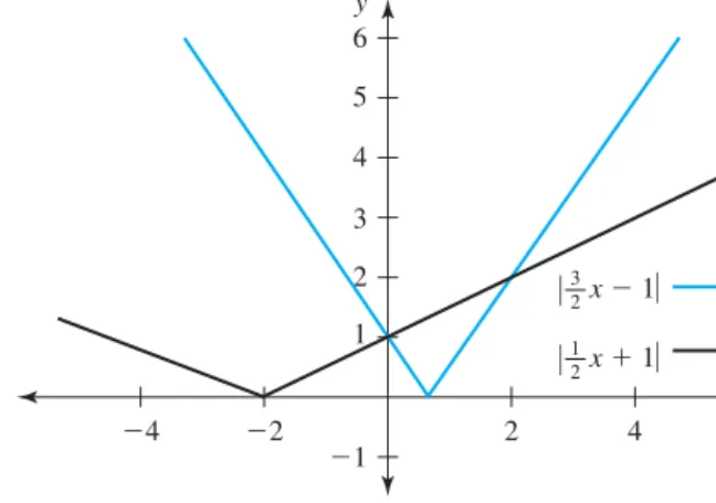
EXAMPLE 2 Solve|32x−1| = |12x+1|.
Solution
Either3
2x−1= 1 2x+1 x =2
or
3
2x−1= − 1
2x+1
3
2x−1= −1 2x−1 2x=0
x=0 A graphical solution of this example is shown in Figure 1.3.
Returning to Example 1, where we found the two points whose distance from 4 was equal to 2, we can also try to find those points whose distance from 4 is less than (or greater than) 2. This amounts to solving inequalities with absolute values.
Looking back at Figure 1.2, we see that the set ofx-values whose distance from 4 is less than 2 (i.e.,|x−4|<2) is the interval(2,6). Similarly, the set ofx-values whose distance from 4 is greater than 2 (i.e.,|x−4| >2) is the union of the two intervals (−∞,2)and(6,∞), or(−∞,2)∪(6,∞).
4 2 2 4 1
1 2 3 4 5 6
x y
x 1
3
2 x 1
1
2
Figure 1.3 The graphs ofy= |32x−1|andy= |12x+1|. The points of intersection are atx=0 andx=2.
In general, to solve absolute-value inequalities, the following two properties are useful:
Letb>0. Then
1. |a|<bis equivalent to−b<a<b. 2. |a|>bis equivalent toa>bora<−b.
EXAMPLE 3 (a) Solve|2x−5|<3. (b) Solve|4−3x| ≥2.
Solution
(a) We rewrite|2x−5|<3 as−3<2x−5<3 Adding 5 to all three parts, we obtain
2<2x<8 Dividing the result by 2, we find that
1<x <4
The solution is therefore the set{x : 1 < x < 4}. In interval notation, the solution can be written as the open interval(1,4).
(b) To solve|4−3x| ≥2, we go through the following steps:
4−3x ≥2
−3x ≥ −2 x ≤ 2
3
or
4−3x ≤ −2
−3x ≤ −6 x ≥2
The solution is the set{x :x ≥2 orx≤ 23}, or, in interval notation,(−∞,23]∪[2,∞).
1.1.2 Lines in the Plane
We will frequently encounter situations in which the relationship between quantities can be described by alinear equation. For example, when a weight is attached to a helical spring made of some elastic material (and the weight is not too heavy), the relationship between the lengthyof the spring and the weightxis
y= y0+kx (1.1)
wherey0denotes the length of the spring when no weight is attached to it andkis a positive constant. Equation (1.1) is an example of a linear equation, and we say that x andysatisfy a linear equation.
Thestandardform of a linear equation is given by Ax+By+C =0
whereA,B, andCare constants,AandBare not both equal to 0, andxandyare the two variables. In algebra, you learned that the graph of a linear equation is a straight line.
If the two points(x1,y1)and(x2,y2)lie on a straight line, then theslopeof the line is
m = y2−y1
x2−x1
(See Figure 1.4.) Two points (or one point and the slope) are sufficient to determine x
y
(x2, y2)
(x1, y1) y2 y1
x2 x1
Figure 1.4 The slope of a straight line.
the equation of a straight line.
If you are given one point and the slope, you can use thepoint–slopeform of a straight line to write its equation, given by
y−y0=m(x−x0)
wheremis the slope and(x0,y0)is a point on the line. If you are given two points, first compute the slope and then use one of the points and the slope to find the equation of the straight line in point–slope form.
Lastly, the most frequently used form of a linear equation is theslope–intercept form
y=mx+b
wheremis the slope andbis they-intercept, which is the point of intersection of the line with they-axis; they-intercept has coordinates(0,b).
We summarize these three forms of linear equations in the following box:
Ax+By+C =0 (Standard Form) y−y0=m(x−x0) (Point–Slope Form)
y=mx+b (Slope–Intercept Form)
EXAMPLE 4 Determine, in slope–intercept form, the equation of the line passing through(−2,1) and(3,−12).
Solution
The slope of the line ism = y2−y1
x2−x1 = −12−1 3−(−2) = −32
5 = − 3 10 Using the point–slope form with(−2,1), we find that
y−1= − 3
10(x−(−2)) or, in slope–intercept form,
y= − 3 10x+ 2
5
We could have used the other point,(3,−12), and obtained the same result.
We now recall two special cases that we illustrate in Figure 1.5:
x h
y k y
h x k
Figure 1.5 The horizontal liney=k and the vertical linex =h.
y=k horizontal line (slope 0) x =h vertical line (slope undefined)
In the next example, we show how to determine the slope and they-intercept of a given straight line.
EXAMPLE 5 Determine the slope and they-intercept of the line 3y−2x+9=0.
Solution
We solve foryin 3y =2x−9. We obtainy= 23x−3. We can now read off the slope m = 23 and they-interceptb= −3.When two quantitiesxandyare linearly related so that y=mx
we say thatyisproportionaltox, withmdenoting theconstant of proportionality, and we write
y∝x
The symbol∝is read “is proportional to.” If we write Equation (1.1) in the form y−y0=kx
then the change in lengthy−y0is proportional to the attached weight with constant of proportionalityk, and we can write
y−y0 ∝x
There are two more properties of straight lines we wish to mention. When two linesl1andl2in the plane have no points in common or are identical, they are called parallel, denoted byl1l2. The following criterion is useful in deciding whether two lines are parallel: Two noncoincident linesl1andl2are parallel (l1 l2) if and only if their slopes are identical. For two noncoincident, nonvertical linesl1 andl2 with slopesm1andm2, respectively, the criterion becomes
l1 l2 if and only if m1=m2
Two linesl1 andl2 are calledperpendicular(l1 ⊥ l2) if their intersection forms an angle of 90◦. The following criterion is useful for deciding whether two lines are perpendicular: Two nonvertical lines are perpendicular if and only if their slopes are negative reciprocals. That is, ifl1andl2are nonvertical lines with slopesm1andm2, then
l1 ⊥l2 if and only if m1m2= −1 We will prove this result in Problem 54 at the end of this section.
1.1.3 Equation of the Circle
Acircleis the set of all points at a given distance, called theradius, from a given point, called thecenter. Ifr is the distance from(x0,y0)to(x,y)(see Figure 1.6), then, using the Pythagorean theorem, we find that
r2=(x−x0)2+(y−y0)2 Ifr =1 and(x0,y0)=(0,0), the circle is called theunit circle.
y
x0 y0
x r
(x, y)
Figure 1.6 Circle with radiusr centered at(x0,y0).
EXAMPLE 6 Find the equation of the circle with center(2,3)and passing through(5,7).
Solution
Using the Pythagorean theorem, we can compute the distance in the plane between (2,3)and(5,7):(5−2)2+(7−3)2=
9+16=5 Thus, this circle has radius 5 and center(2,3), and its equation is
25=(x−2)2+(y−3)2
1.1.4 Trigonometry
We will need a few results from trigonometry. Recall that angles are measured in y
y
x x
sin u (x, y)
tan u
cos u u 1
1 1
Figure 1.7 The trigonometric functions on a unit circle.
either degrees or radians and that a complete revolution on a unit circle (Figure 1.7) corresponds to 360◦, or 2π. For reasons that will become clear, the radian measure is preferred in calculus. To convert between degree and radian measure, we use the formula
θmeasured in degrees
360◦ = θmeasured in radians 2π
For instance, to convert 23◦into radian measure, we compute θ =23◦ 2π
360◦ =0.401 To convertπ6 into degrees, we compute
θ = π 6
360◦ 2π =30◦
There are four trigonometric functions that you should be familiar with: sine, cosine, tangent, and secant; the other two, cotangent and cosecant, are rarely used.
The six are defined on a unit circle (see Figure 1.7) and are abbreviated as sin, cos, tan, sec, cot, and csc, respectively. Recall that a positive angle is measured counter- clockwise from the positivex-axis, whereas a negative angle is measured clockwise.
The six trigonometric functions are defined as follows:
sinθ= y
1 =y cscθ= 1 sinθ = 1
y cosθ= x
1 =x secθ= 1 cosθ = 1
x tanθ= y
x cotθ= 1
tanθ = x y
There are a number of frequently used trigonometric identities. First, since tanθ = y/xwithy =sinθandx=cosθ, it follows that
tanθ = sinθ cosθ
Now, applying the Pythagorean theorem to the triangle in Figure 1.7 and using the notation sin2θ =(sinθ)2, we find that
sin2θ+cos2θ =1
Next, if we divide the preceding identity by cos2θ, we obtain sin2θ
cos2θ +1= 1 cos2θ
Using tanθ =sinθ/cosθand secθ =1/cosθ, we can write this as tan2θ+1=sec2θ
In the next example, we solve a trigonometric equation.
EXAMPLE 7 Solve
2 sinθcosθ =cosθ on[0,2π)
Solution
We should not be tempted to cancel cosθ on each side; this would cause us to lose solutions. Instead, we bring cosθto the left side and factor cosθto obtaincosθ(2 sinθ−1)=0 That is,
cosθ =0 or 2 sinθ−1=0 Solving cosθ =0, we find that
θ = π
2 or θ = 3π
2 Solving 2 sinθ−1=0, we get
sinθ = 1 2 which yields
θ = π
6 or θ = 5π
6 The solution set is therefore{π6,π2,5π6,3π2 }.
Figure 1.8 yields the following two identities when we compare the two angles
x y
u u
(cos u, sin u)
(cos(u), sin(u)) Unit circle
1
1
Figure 1.8 Using the unit circle to define trigonometric identities.
θ and−θ (a positive angle is measured counterclockwise from the positivex-axis, whereas a negative angle is measured clockwise):
sin(−θ)= −sinθ and cos(−θ)=cosθ
Some exact trigonometric values are collected in Table 1-1. Of course,12 0=0,
1 2
1= 12, and12
4=1, and you should memorize these simplified values. Rewriting Table 1-1 will make it easier to re-create the table in case you forget the exact values.
Using tanθ =sinθ/cosθ, you immediately get the values for tanθ. TABLE 1-1 Some Exact Trigonometric Values
Angleθ 0 π
6
π 4
π 3
π 2 (0◦) (30◦) (45◦) (60◦) (90◦)
sinθ 1
2
0 1 2
1 1 2
2 1 2
3 1 2
4
cosθ 1
2
4 1 2
3 1 2
2 1 2
1 1 2
0
1.1.5 Exponentials and Logarithms
Exponentials and logarithms are particularly important in biological contexts.
An exponential is an expression of the form ar
whereais called thebaseandr theexponent. Unlessr is an integer or unlessr is a rational number of the formp/qwherepis an integer andqis an odd integer, we will assume thatais positive. We summarize some of the properties of an exponential as follows:
aras =ar+s (ab)r =arbr ar
as =ar−s
a b
r
= ar br a−r = 1
ar ars
=ar s
EXAMPLE 8 Evaluate the following exponential expressions:
(a) 3235/2=32+5/2 =39/2 (b) 2−423
22 = 2−1
22 =2−1−2=2−3= 1 23 = 1
8 (c) aka3k
a5k =ak+3k−5k =a−k = 1 ak
Logarithms allow us to solve equations of the form 2x =8
The solution of this equation isx =3, which we can write as x =log28=3
In other words, a logarithm is an exponent. The expression logay
is the exponent on the baseathat yields the numbery. Logarithms are defined only fory >0 (where the base is assumed to be positive and different from 1). We have the following correspondence between logarithms and exponentials:
x=logay is equivalent to y=ax
EXAMPLE 9 Which real numberxsatisfies
(a) log3x = −2? (b) log1/28=x?
Solution
(a) We write this in the equivalent form x=3−2 Hence,x = 1 32 = 1
9 (b) We write this in the equivalent form
1 2
x
=8 2−x =23
2x =2−3
Setting the exponents equal to each other, we find thatx = −3. Note that, in order to compare exponents, the bases must be the same.
Some important properties of logarithms are as follows:
loga(x y)=logax+loga y loga
x y
=logax−loga y logaxr =rlogax
The most important logarithm is the natural logarithm, which has the number eas its base. The number eis an irrational number whose value is approximately 2.7182818. The natural logarithm is written lnx; that is, logex=lnx.
EXAMPLE 10 Assume thatxandyare positive, and simplify the following expressions:
(a) log3(9x2)=log39+log3x2=2+2 log3x
(b) log5 x25x+3 =log5(x2+3)−log55−log5x =log5(x2+3)−1−log5x [Note that log5(x2+3)cannot be simplified any further.]
(c) −ln12 =ln(12)−1=ln 2 (d) ln3x√2
y =ln 3+lnx2−ln√
y=ln 3+2 lnx−12lny (In the last step, we used the fact that√
y =y1/2.)
In algebra, you learned how to solve equations of the forme2x =3 or ln(x+1)= 5. We will need to do this frequently. The key to solving such equations are the two identities
logaax= x and alogax =x
The next example illustrates how to use these identities.
EXAMPLE 11 Solve forx.
(a) e2x =3 (b) ln(x+1)=5 (c) 52x−1=2x
Solution
(a) To solvee2x =3 forx, we take logarithms to baseeon both sides:lne2x =ln 3 But lne2x =2x; hence,
2x =ln 3, or x = 1 2ln 3
(b) To solve ln(x+1)=5, we write the equation in exponential form:
eln(x+1) =e5 This simplifies to
x+1=e5, or x =e5−1
(c) To solve 52x−1 = 2x forx, we observe that the two bases are different. We therefore cannot compare the exponents directly. Instead, we take logarithms on both sides. Any positive base (different from 1) for the logarithm would work, and we choose basee, since it is the most commonly used base in calculus. Doing so yields
ln 52x−1=ln 2x or, after simplifying,
(2x−1)ln 5=xln 2 Solving forx, we find that
2xln 5−xln 2=ln 5 x(2 ln 5−ln 2)=ln 5 Hence,
x= ln 5 2 ln 5−ln 2
1.1.6 Complex Numbers and Quadratic Equations
The square of a real number is always nonnegative. However, there are situations in which we need to take a square root of a negative number. Since the resulting square root cannot be a real number, we introduce a new symbol, which we denote byi, that will allow us to deal with this case. We set
i2= −1
The symboliis called theimaginary unit. Thus, instead of writing
−17, for instance, we can now writei
17.
The symboli allows us to introduce a new number system, the set of complex numbers:
Acomplex numberis a number of the form z =a+bi
whereaandbare real numbers. The real numberais thereal partofa+bi, and the real numberbis theimaginary part.
For instance,−3+7ihas real part−3 and imaginary part 7, and 2−5i has real part 2 and imaginary part−5. Sincea+0i =a, it follows that the set of real numbers is a subset of the set of complex numbers. Complex numbers of the formbi are called purely imaginary numbers.
Two complex numbers are equal if their respective real and imaginary parts are equal; that is,
a+bi =c+di if and only if a=c and b=d To add two complex numbers, we use the following rule:
(a+bi)+(c+di)=(a+c)+(b+d)i
This rule says that real and imaginary parts are added separately. To calculate the product of two complex numbers, we proceed as follows:
(a+bi)(c+di)=ac+adi+bci+bdi2
=ac+(ad+bc)i−bd
=(ac−bd)+(ad+bc)i
Note that we usedi2= −1 in the penultimate step. There is no need to memorize the product of two complex numbers, since we can always compute it by the distributive law.
EXAMPLE 12 Find
(a) (2+3i)−(5−6i), (b) (5−3i)(1+2i).
Solution
(a) (2+3i)−(5−6i)=2+3i−5+6i = −3+9i,(b) (5−3i)(1+2i)=5+10i −3i−6i2=5+7i−(6)(−1)=11+7i.
Ifz=a+bi is a complex number, itsconjugate, denoted byz, is defined as z =a−bi