Scenarios of methane emission reductions to 2030:
abatement costs and co-benefits to ozone air quality and human mortality
J. Jason West&Arlene M. Fiore&Larry W. Horowitz
Received: 20 February 2011 / Accepted: 12 February 2012 / Published online: 7 March 2012
#Springer Science+Business Media B.V. 2012
Abstract Methane emissions contribute to global baseline surface ozone concentrations;
therefore reducing methane to address climate change has significant co-benefits for air quality and human health. We analyze the costs of reducing methane from 2005 to 2030, as might be motivated to reduce climate forcing, and the resulting benefits from lower surface ozone to 2060. We construct three plausible scenarios of methane emission reductions, relative to a base scenario, ranging from 75 to 180 Mton CH4yr−1decreased in 2030. Using compilations of the global availability of methane emission reductions, the least aggressive scenario (A) does not incur any positive marginal costs to 2030, while the most aggressive (C) requires discovery of new methane abatement technologies. The present value of implementation costs for Scenario B are nearly equal to Scenario A, as it implements cost-saving options more quickly, even though it adopts positive cost measures. We estimate the avoided premature human mortalities due to surface ozone decreases by combining transient full-chemistry simulations of these scenarios in a global atmospheric chemical transport model, with concentration-mortality relationships from a short-term epidemiologic study and projected global population. An estimated 38,000 premature mortalities are avoided globally in 2030 under Scenario B. As benefits of methane reduction are positive but costs are negative for Scenario A, it is justified regardless of how avoided mortalities are valued. The incremental benefits of Scenario B also far outweigh the incremental costs.
Scenario C has incremental costs that roughly equal benefits, only when technological
Electronic supplementary material The online version of this article (doi:10.1007/s10584-012-0426-4) contains supplementary material, which is available to authorized users.
J. J. West (*)
Department of Environmental Sciences and Engineering, University of North Carolina at Chapel Hill, CB#7431, Chapel Hill, NC 27599, USA
e-mail: [email protected] A. M. Fiore
:
L. W. HorowitzGeophysical Fluid Dynamics Laboratory, National Oceanic and Atmospheric Administration, 201 Forrestal Road, Princeton, NJ 08540, USA
Present Address:
A. M. Fiore
Lamont-Doherty Earth Observatory, 61 Route 9W, Palisades, NY 10964, USA
learning is assumed. Benefits within industrialized nations alone also exceed costs in Scenarios A and B, assuming that the lowest-cost emission reductions, including those in developing nations, are implemented. Monetized co-benefits of methane mitigation for human health are estimated to be $13–17 per ton CO2eq, with a wider range possible under alternative assumptions. Methane mitigation can be a cost-effective means of long-term and international air quality management, with concurrent benefits for climate.
1 Introduction
Emissions of methane (CH4) related to human activities have caused global atmospheric methane concentrations to more than double since the preindustrial period, causing a positive radiative climate forcing that is second only to CO2(Forster et al.2007). In addition to being a greenhouse gas, methane also reacts in the atmosphere to produce ozone (Crutzen1973). Since methane is long-lived in the atmosphere (a perturbation lifetime of 12 years, Forster et al.2007), it affects global baseline (i.e., not affected by local sources) concentrations of ozone (Wang and Jacob1998). In fact, methane is the dominant anthropogenic volatile organic compound (VOC) contributing to ozone formation in the global troposphere (Fiore et al.2002). Anthropogenic increases in emissions of methane and nitrogen oxides (NOx) have been identified as the most important causes for the historic increases in background ozone concentrations since preindus- trial times (Wang and Jacob1998; Lelieveld and Dentener2000).
Reductions in methane emissions to address climate change therefore have significant co- benefits for improving air quality and human health globally, regardless of where those reductions occur (Hansen et al.2000; Fiore et al.2002). These co-benefits, however, have received little attention (West et al. 2006). In contrast, the co-benefits of mitigating CO2
emissions for air quality and human health have been analyzed extensively, with the majority of these studies finding that air pollution co-benefits are significant in comparison with the costs of mitigation or monetized benefits of slowing climate change (Ekins1996; WGPHFFC1997;
OECD2000; Cifuentes et al.2001a,b; Syri et al.2001; Hourcade et al.2001; Burtraw et al.
2003; Aunan et al.2003,2004; Vennemo et al.2006; van Vuuren et al.2006a; Barker et al.
2007). Co-benefits of CO2mitigation are realized via reductions in air pollutants co-emitted with CO2. In contrast, co-benefits of methane mitigation are realized through reactions that methane participates in directly. In addition, methane emissions are expected to grow, partic- ularly from developing nations, and several measures are known to reduce methane emissions at low cost (Nakicenovic et al.2000; IEA2003; EPA2006a; EPA2006b; Moss et al.2010).
Including methane reductions in has been shown to reduce overall costs of multi-gas GHG reduction programs (Reilly et al. 1999; Weyant et al. 2006; van Vuuren et al. 2006b).
Consequently, methane mitigation has increasingly been included in discussions of long-term planning for ozone management (EMEP 2005; Royal Society 2008; HTAP 2010), in addition to its role as an important forcing agent with a short lifetime (Jackson 2009;
UNEP 2011).
We previously analyzed the potential for reducing global baseline ozone as a function of the costs of identified methane controls, and presented the strengths and weaknesses of managing ozone through methane reductions relative to more traditional ozone precursors—
NOx, VOCs, and carbon monoxide (West and Fiore 2005). We also showed that among reductions in these four ozone precursors to improve ozone air quality, reducing methane best decreases climate forcing (West et al.2007a). Finally, we simulated an immediate 20%
global reduction of anthropogenic methane emissions and showed that the monetized co- benefits of avoided premature mortalities from reduced ozone are comparable to previous
estimates of co-benefits for CO2, and can exceed the costs of methane control, suggesting that this reduction could be justified for ozone air quality purposes alone (West et al.2006).
In this study, we reevaluate the costs and benefits of reducing methane emissions, using realistic future scenarios of methane abatement. We present here three plausible scenarios of global methane emissions abatement relative to a base scenario to 2030, which are based on compilations of the global potential for methane abatement. These scenarios were modeled by Fiore et al. (2008) in fully transient 25-year simulations using the MOZART-2 model of global atmospheric chemistry and transport, to assess future concentrations of methane and ozone, and as a bounding case, we also consider a complete removal of anthropogenic methane emissions in 2030. The changes in surface ozone concentrations from these simulations are used here to estimate the global avoided premature mortalities, and these benefits are compared with the estimated costs of methane emission control.
2 Base methane emissions and abatement scenarios
Anthropogenic emissions of methane derive from many source categories, including energy production and distribution (in the coal, oil, and natural gas sectors), landfills, and wastewater treatment. Agricultural operations also contribute substantially to current anthropogenic emis- sions, mainly in the production of rice and ruminant animals (mainly cows) (Denman et al.
2007). Because methane is the main component of natural gas, several actions that capture methane for energy use involve a net cost-savings or small positive cost. While these cost-saving actions have increasingly been adopted in industrialized countries, causing emissions from these countries to decrease since 1990 (EPA2006a), they are much less widespread elsewhere, and recent estimates suggest that roughly 10% of current global anthropogenic emissions can be reduced at a net cost-savings using presently available technology (IEA2003; EPA2006b).
Here we construct three plausible and illustrative scenarios of future methane emissions abatement over the period 2005 to 2030, relative to a base scenario, the IIASA Current Legislation (CLE) scenario (Dentener et al. 2005; Cofala et al. 2007).
The CLE scenario projects global anthropogenic methane emissions to increase by 40%
between 2000 and 2030, an increase that falls in the middle of the Intergovernmental Panel on Climate Change (IPCC) Special Report on Emissions Scenarios (SRES) scenarios (Nakicenovic et al. 2000).
Relative to this base scenario, three scenarios of methane emission reductions are developed beginning in 2005. These scenarios use as benchmarks studies of the global availability of methane emission reductions using current technologies by 2030: the IIASA Maximum Feasible Reduction (MFR) scenario (Dentener et al.2005; Cofala et al.2007), and compilations of the global availability of methane emission reductions as a function of cost by the International Energy Agency (IEA2003) and the US Environmental Protection Agency (EPA 2006b). The IEA (2003) and EPA (2006b) report the technical costs of implementation, including capital costs, operation and maintenance, and avoided costs from the recovery of methane, but omit transaction costs, such as the costs to administer a methane reduction strategy. They created marginal abatement cost curves for annualized costs under assumptions of a discount rate (10% per year), future energy prices, and for the EPA, a tax rate that applies to corporations considering methane reductions (40%).
For our purpose of comparing social costs and benefits, we apply a more appropriate social discount rate of 5% per year and no tax rate, and adjust cost estimates accordingly.
Both the IEA (2003) and EPA (2006b) report costs in US dollars for the year 2000, and we use these units here.
Figure1shows global methane abatement in the three benchmark studies and the three methane reduction scenarios developed here. The MFR scenario is intended to be an aggressive scenario which immediately deploys all currently-available methane reduction technologies, even though some are costly, but assumes no future discovery of new abatement technologies (Dentener et al. 2005). Methane reductions under IEA and EPA are shown in 2030 for marginal costs of $15 per ton of CO2equivalent (CO2eq) reduced, as this is roughly the monetized benefit of reducing methane estimated in previous studies of benefits for human mortality (West et al.2006) and other benefits to health, agriculture, and forestry (West and Fiore2005). Throughout this paper, we use a 100-year global warming potential for methane of 21, the value currently used in emission trading markets, such that 1 ton of CH4 equals 21 tons of CO2eq.
The IEA (2003) reported base results as the global availability of methane reductions in 2010 at a 10% discount rate, using current technologies in five sectors: coal, oil, gas, wastewater, and landfills. We use their sensitivity case for 2020, and adjust the cost curve by multiplying by the ratio of available reductions in other reported sensitivity cases (relative to the base) for a 5% discount rate and twice the base energy price. Because these reported sensitivity cases are based on original data on the time profile of costs for each abatement measure, the error in our extrapolation is low. We then add global abatement opportunities in
0 20 40 60 80 100 120 140 160 180 200
CH4(Tgyr-1)CH4(Tgyr-1)
0 50 100 150 200 250 300 350 400 450 500
2000 2005 2010 2015 2020 2025 2030
2000 2005 2010 2015 2020 2025 2030
a
b
Scen A Scen B Scen C MFR EPA IEA
CLE Scen A Scen B
Scen C MFR RCP8.5
RCP6.0 RCP4.5 RCP2.6
Fig. 1 aMethane emissions reductions relative to the base CLE scenario, andbtotal anthropogenic emissions, for the CLE base and MFR scenarios, available reductions at <$15 per ton CO2equivalent for the IEA and EPA compilations of global methane abatement opportunities (extended to 2030 and modified as described in the text), three scenarios defined in this study, and the RCP scenarios
agricultural sources (manure management, enteric fermentation, and rice cultivation) as reported by DeAngelo et al. (2006) and EPA (2006b) for 2020. Finally, we extrapolate these results to 2030 proportionally to the growth in base scenario methane emissions. Accounting for these changes gives a global availability of about 79 Mton CH4yr−1in 2030 at a negative marginal cost, and 122 Mton CH4yr−1in 2030 at <$15 per ton CO2eq (Fig.1a).
The EPA (2006b) reports global methane reductions available for four industrial sectors (coal, oil, natural gas, and landfills), and three agricultural sectors (manure management, enteric fermentation, and rice cultivation), in 2020, which we extrapolate to 2030 as for IEA (2003). The EPA (2006b) reports generally lower availability of methane reductions than does IEA (2003). The reductions from agriculture for EPA (2006b) are the same that we added to the results from IEA (2003); consequently, the major difference is that EPA (2006b) does not include possible reductions in wastewater treatment, which is a large source of cost-effective reductions for IEA (2003). The EPA (2006b) does not report the sensitivity of their results at a 5% discount rate, 0% tax rate, or at a higher energy price, but clearly, changing these assumptions in line with our assumptions above for IEA would increase the availability of methane reductions at a given cost. Because of these inconsistencies, we do not use EPA (2006b) estimates in forthcoming sections.
In Fig.1, Scenario A is constructed such that it clearly can be achieved for less than $15 per ton CO2eq marginal cost, and is well within the reductions considered possible in the MFR scenario. Under Scenario B, the 2030 reduction roughly equals the global available reduction at <$15 per ton CO2eq of IEA (2003), after modifying the IEA (2003) marginal cost curves as described above. Scenario B is also possible according to the MFR scenario, but exceeds the available reductions of EPA (2006b). Scenario C cannot be achieved using only the technologies included in the MFR, IEA, or EPA datasets, requiring development of new technologies before 2030.
These three scenarios span a range of methane emission reductions, with totals of 75, 125 and 180 Mton yr−1in 2030 from Scenarios A, B, and C, respectively, which are 18%, 29%
and 42% of global anthropogenic CLE emissions in 2030. Total anthropogenic methane emissions (Fig.1b) would stabilize under Scenario A at slightly more than 2005 emissions, while Scenarios B and C would decrease emissions relative to 2005. These scenarios are also compared with the new Representative Concentration Pathway scenarios (Moss et al.2010), which show a wider range of 2030 emissions, with the no-policy scenario (RCP8.5) growing faster than CLE, and the aggressive policy scenario (RCP2.6) reaching lower emissions than Scenario C.
The marginal costs of each of these scenarios are shown in Fig.2, based on IEA (2003) data, modified as described above, and assuming that measures are applied strictly from the least costly alternatives to the most costly. Estimating the true time profile of costs is not entirely possible, as the IEA (2003) and EPA (2006b) report annualized costs. In many cases, these projects involve large capital costs at the beginning of the project. Since it is not possible to reconstruct the actual cost history, we report the annual costs (as if the investment were financed with a loan) over the lifetime of the technology, but this approach will tend to underestimate the actual costs early in the period analyzed. The lifetimes of these technol- ogies range from 5 to 30 years (IEA2003; EPA2006b) and we assume that each technology can be replaced at the end of its lifetime with another at the same annual cost, as would generally be expected.
In Fig.2, we project the marginal cost in each year assuming no technological learning through 2030. This assumption is conservative, as we expect the costs of individual technologies to decrease through time and new technologies make greater emission reduc- tions possible. Scenario A has a 2030 marginal cost of $0 per ton CH4, assuming no
technological learning. Likewise, under Scenario B, marginal costs remain less than or equal to $0 until 2017. Scenario C incurs very high marginal costs in 2021 and 2022 (>$1500 per ton), incorporating the most costly measures in IEA (2003), and becomes infeasible in 2023 when available technologies are exhausted.
Scenario C could be possible with an increase in methane abatement opportunities through technological innovation. The existing literature on innovation, including for emission controls, has focused on a single type of technology and the reduction in marginal cost as that technology matures (Dutton et al.1984; Grubb et al.2002; Taylor et al.2003;
Rubin et al.2004; Riahi et al.2004; EPA, 2006b). Here we are more interested in how innovation will increase the availability of emission reductions from a suite of many possible technologies through time, rather than the decrease in cost of one technology, especially as Scenario C is not possible using identified technologies at any cost. Experience has shown that after beginning to control emissions of a pollutant, innovation both decreases the costs per ton reduced and increases the emission reductions possible below a given marginal cost.
However, the current literature does not provide a good basis for quantifying the growth in emission reduction potential through time from an expanding suite of technologies.
Methane abatement costs are therefore presented both without and with technological learning. Lacking historical evidence on which to base our assumptions for learning, we consider the rate of growth in emission reduction potential that would be required to make Scenario C possible. We define emission reduction potential as the available emission reduction from all known technologies at or less than a given marginal cost; in a future year, it is the available reductions plus those reductions that have been implemented between the present and the future year. We therefore assume a growth rate of emission reduction potential that applies to reductions at each marginal cost; in doing so, we expand the reductions available at each cost, but conservatively ignore the likelihood that the marginal costs of each individual technology will decrease through time (shifting the cost curve right, but not down). We find that a 1% per year growth rate in the emission reduction potential is more than sufficient to make Scenario C possible; this growth rate is not unreasonable should aggressive policies for methane mitigation be instituted. In Fig.2, assuming techno- logical learning decreases the marginal costs of Scenarios A and B, particularly in the 2020s, and Scenario C becomes feasible with a 2030 marginal cost of $859 per ton CH4($40.9 per ton CO2eq). Many projections of future emissions over the next century must assume
-1500 -1000 -500 0 500 1000 1500
2005 2010 2015 2020 2025 2030 Marginal cost ($/tonCH4)
Scen A Scen B Scen C Fig. 2 Marginal cost of methane
emission reduction scenarios to 2030, based on the marginal costs reported by IEA (2003) and modified as described in the text, for no technological learning (solid), and learning to expand the emission reductions possible at each marginal cost by 1% per year (dashed). These costs can be divided by the global warming potential of methane, to obtain costs per ton CO2eq
technological innovation, and our assumption of Scenario C in 2030 is in line with global methane emissions in recent scenarios with aggressive climate policies (e.g., for RCP2.6 in Fig.1; Clarke et al.2006; Moss et al.2010).
Because of the long atmospheric lifetime of methane, the benefits of reduced ozone are realized over decades. Accordingly, we evaluate scenarios to 2060 in order to fully account for the costs and benefits of all implemented actions. Here we assume that annual costs of implementation in 2030 are constant to 2060, assuming that the same technologies continue to be applied, and with no further innovation beyond 2030 in the case of technological learning.
3 Changes in surface ozone concentrations due to methane abatement
The CLE base scenario and these three methane abatement scenarios were simulated by Fiore et al. (2008) using MOZART-2 in fully transient simulations to 2030, with emissions of all other species following the CLE scenario (Dentener et al.2005; Cofala et al.2007).
Fiore et al. (2008) report the difference in surface ozone concentrations between CLE and the three methane reduction scenarios, as well as the radiative climate forcing. Here we present the changes in population-weighted ozone concentration in several world regions, as these indicators are more directly relevant for human health.
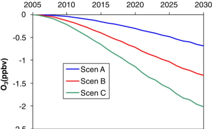
Figure 3 shows the decreases in the global annual average population-weighted 8-hr.
daily maximum ozone under the three methane reduction scenarios. Relative to the base scenario, ozone concentration decreases smoothly in each scenario, reaching global average reductions of 0.7, 1.3, and 2.0 ppb in 2030 for Scenarios A, B, and C, respectively. In Table1, the changes in ozone are shown for individual world regions defined in FigureS1.
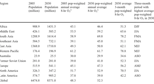
Table 1 shows the population-weighted ozone concentrations in the base simulation, as averages annually and in the “ozone season” in each region, which is defined as the three-month period with the greatest average population-weighted 8-hr. daily maximum ozone concentration in 2030. In 2005, the Western Pacific region has the highest population-weighted annual average 8-hr. ozone, followed by South Asia and the Middle East. From 2005 to 2030, ozone in the base scenario increases markedly in South Asia, such that it is the region with highest ozone in 2030, as well as in Southeast Asia and the Middle East. The ozone growth in these regions is consistent
-2.5 -2 -1.5 -1 -0.5 0
2005 2010 2015 2020 2025 2030
O3(ppbv)
Scen A Scen B Scen C Fig. 3 Change in global annual
average population-weighted 8-hr. ozone, in the three methane reduction scenarios relative to the CLE baseline
with other models that analyzed the CLE scenario (Dentener et al.2006), and is due to large projected increases in emissions in these regions and the large sensitivity to changes in emissions in tropical regions (West et al. 2009a). Industrialized nations show much less growth in ozone as a result of planned emission reductions included in CLE.
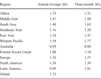
Reducing methane (Table2) causes the greatest decrease in surface ozone in the Middle East, in agreement with previous results (West and Fiore2005; West et al.2006; Fiore et al.
2008). The Western Pacific, South Asia, and Europe also see ozone decreases greater than the global average. We find that the regional pattern of the response to changes in methane
Table 1 Population and surface ozone concentrations (in ppb) in the base simulation, in each of 11 world regions and globally
Region 2005
Population (million)
2030 Population (million)
2005 pop-weighted annual average 8-hr O3
a
2030 pop-weighted annual average 8-hr O3
a
2030 average 3-month pop-weighted 8-hr O3
Three-month period with highest average pop-weighted 8-hr O3in 2030
Africa 908.9 1431.5 43.1 46.4 51.3 DJF
Middle East 426.1 585.2 53.5 59.2 65.6 JJA
South Asia 1288.9 1614.4 58.9 69.8 78.2 FMA
Southeast Asia 584.5 732.1 39.1 45.0 51.1 FMA
East Asia 1368.0 1710.8 49.3 50.8 62.1 MJJ
Western Pacific 176.4 196.9 61.2 61.7 78.8 MJJ
Australia 23.9 25.5 30.0 29.9 34.6 ASO
Former Soviet Union 281.0 281.0 39.0 41.0 52.3 JJA
Europe 515.9 541.1 45.1 47.3 56.2 AMJ
North America 326.3 347.2 51.7 52.9 70.5 JJA
Latin America 574.7 905.2 37.8 39.0 42.2 ASO
Global 6474.8 8371.0 48.3 52.3
aThe 2005 and 2030 results differ in the spatial distribution of population, as well as ozone concentrations. If we use the 2030 population distribution in 2005, the global population-weighted annual average 8-hr O3is 48.0 ppb
Table 2 Decreases in the population-weighted 8-hr.
ozone concentrations (ppb) in 2030 in Scenario B relative to the CLE scenario, for the annual average and average in the three-month period with highest ozone. Changes in ozone for Scenarios A and C follow the same pattern, scaling simply to results for Scenario B (see text)
Region Annual averageΔO3 Three-monthΔO3
Africa 1.33 1.32
Middle East 1.67 1.98
South Asia 1.48 1.63
Southeast Asia 1.16 1.20
East Asia 1.34 1.47
Western Pacific 1.54 1.77
Australia 0.89 0.86
Former Soviet Union 1.08 1.34
Europe 1.36 1.57
North America 1.26 1.38
Latin America 0.99 1.01
Global 1.33
emissions is nearly the same in the three scenarios (Fiore et al.2008). The global average ozone change in Scenario A is 52% of that in Scenario B, and the results in each individual region and season are also very nearly 52% of those in Scenario B. Likewise, changes in ozone in Scenario C are very nearly 152% that in Scenario B in all regions and seasons.
Fiore et al. (2008) also present the steady-state change in ozone where anthropogenic emissions are eliminated (by fixing methane globally to the preindustrial concentration of 700 ppb). The global population-weighted annual average 8-hr. daily maximum ozone decreases by 5.6 ppb, which would be the greatest ozone reduction possible by reducing methane emissions. If we assume that anthropogenic emissions of methane are eliminated starting in 2006, methane would not have reached the preindustrial concentration by 2030, nor would ozone have reached steady state. Using the perturbation lifetime of methane of 11.3 years diagnosed for MOZART-2 (Fiore et al.2008), 89% of this steady state change would be achieved by 2030, giving a reduction in the global population-weighted annual average 8-hr. daily maximum ozone of 5.0 ppb, and we estimate ozone changes between 2005 and 2030 similarly. The spatial pattern of the surface ozone change does not differ substantially with the other scenarios, as the change in ozone in 2030 from eliminating anthropogenic methane emissions is roughly 3.75 times that in Scenario B. These relation- ships between methane and surface ozone concentrations are consistent with others in the literature (Fiore et al.2008). A multimodel study finds that responses of surface ozone to changes in methane vary among 18 models by a coefficient of variation (σ/μ) of 20%, and that MOZART-2 is not an outlier (Fiore et al.2009).
We evaluate changes in ozone beyond these simulations until 2060, assuming no further changes in emissions of methane or other species, so that benefits can be fully evaluated.
Here we calculate the steady-state methane calculation corresponding to the methane emissions in 2030 in each scenario, and have methane approach this steady state exponentially according to its perturbation lifetime. Changes in ozone are then calculated in each year, grid cell, and day by scaling to the changes in ozone between a present-day simulation (1760 ppb methane) and a methane perturbation simulation (1460 ppb) (Fiore et al. 2008). Scaling to these steady-state simulations is justified, irrespective of changes in base scenario methane and other emissions, as ozone is very nearly linear with methane changes (Fiore et al. 2008).
4 Avoided premature mortalities associated with ozone reductions
Ozone has been associated with premature mortality in a large number of daily time-series epidemiological studies (Levy et al.2001,2005; Thurston and Ito2001; Gryparis et al.2004;
Bell et al.2004,2005; Ito et al.2005; Bell and Dominici2006; NAS 2008). The global avoided premature mortalities associated with modeled ozone reductions are assessed using the general methods of West et al.(2006;2007b;2009b) and Anenberg et al. (2009;2010), which are supported by the US National Academy of Sciences (NAS2008). The relationship between changes in ozone concentration and daily mortalities is derived from a daily time-series study of 95 United States cities (Bell et al.2004), and we use their results for 8-hr. daily maximum ozone. Bell et al.(2004) show a smaller relationship between ozone and mortality than meta-analyses (Bell et al. 2005; Ito et al. 2005; Levy et al.
2005), but we select this study because it is not subject to a possible publication bias (the tendency to selectively publish studies showing stronger relationships). In addition to these results for short-term ozone mortality, Jerrett et al. (2009) find evidence for a relationship between ozone and long-term (chronic) mortality; as there are few other
studies to support long-term ozone mortality, we conservatively limit our estimates to short-term mortality, but note that mortality impacts may be greater had we estimated long-term mortality. While the majority of epidemiologic evidence is derived from studies in the US and Europe, available studies from elsewhere are not inconsistent (HEI Scientific Oversight Committee 2004), and we apply this relationship globally.
Global atmospheric models are now commonly used to drive air pollution health impact assessments (West et al.2006;2007b;2009b; Corbett et al.2007; Jacobson2008; Liu et al.
2009; Anenberg et al. 2009; 2010; Barrett et al. 2010). These studies have important uncertainties due to the coarse resolution of global models. For the present case, these uncertainties are expected to be small, as methane affects the global ozone background and is not expected to play a major role in ozone formation in polluted urban plumes.
Nonetheless, the possible effects of methane on ozone on finer scales, including urban areas (see Fiore et al. 2008), and the uncertainties of coarse grid resolution for health impact analysis, should be investigated more fully.
Population is projected annually into the future in each of four world regions based on the IPCC SRES B2 scenario, in which the global population increases to 8.37 billion in 2030, selected because B2 is near the center of the SRES scenarios (Nakicenovic et al.2000). The spatial distribution of population is from the LandScan database (Oak Ridge National Lab 2005) for the global 2003 population, which is then mapped onto the grid used for atmospheric modeling (1.9°×1.9°). Baseline mortality rates are taken as the“non-accident”
baseline mortality in each of fourteen world regions from WHO (2004). Avoided premature mortalities are calculated using the change in 8-hr. daily maximum ozone concentration between the methane reduction scenario and the base scenario, in each grid cell on each day to 2060. We apply a low-concentration threshold of 25 ppb, below which changes in ozone concentration are not assumed to affect mortality, and compare to results with no threshold.
In Fig.4, the time profile of avoided premature mortalities roughly follows that for ozone (Fig.2), but also reflects the growth in population, with avoided mortalities in 2030 of about 19,500, 37,800, and 57,200, in Scenarios A, B, and C, respectively. Accumulated over the period 2005–2030, 187,000 premature mortalities are avoided in Scenario A, 411,000 in Scenario B, and 644,000 in Scenario C. These results are for a low-concentration ozone
0 10000 20000 30000 40000 50000 60000 70000 80000 90000 100000
2005 2015 2025 2035 2045 2055
Avoided Mortalities per Year
Scen A Scen B Scen C Fig. 4 Global annual avoided
premature mortalities due to ozone, under the three methane emissions abatement scenarios, for total avoided mortalities with a low-concentration
threshold of 25 ppb (solid lines), total mortalities with no low-concentration threshold (dotted lines), and cardiovascular and respiratory mortalities with a 25 ppb threshold (dashed lines)
threshold of 25 ppb; results with no threshold are ~5% higher (Fig. 4). Beyond 2030, avoided mortalities continue to rise, but less slowly, as methane approaches a steady state change and as population continues to grow. We previously showed that ozone mortality has little sensitivity to changes in threshold below about 30 ppb, but that higher thresholds substantially reduce the avoided mortalities (West et al.2006; West et al.2007b). In the scenario where methane emissions are eliminated (not shown) 140,000 mortalities are avoided in 2030 with 2.19 million avoided mortalities between 2005 and 2030, assuming a 25 ppb threshold.
As expected, annual avoided mortalities are small compared to the total annual prema- ture mortalities attributed to ozone (~700,000) and fine particulate matter (~3.7 million) (Anenberg et al. 2010). Across all scenarios, changes in mortality scale roughly proportionally to the changes in ozone concentration, and since the change in ozone is proportional to the methane reduction, mortalities roughly scale with methane.
In Scenario B in 2030, the greatest numbers of avoided premature mortalities are observed to occur in Africa, South Asia, and East Asia (Fig.5and Table3), as these regions are projected to have the greatest population in 2030 (Table1). The avoided mortalities per million people are greatest in Africa, as Africa has the highest baseline mortality rates in the world and experiences a high change in ozone (Table 2). High numbers of avoided premature mortalities per million people are also seen in South Asia, Europe, the Former Soviet Union, Western Pacific, and the Middle East due to large changes in ozone and/or high baseline mortality.
As a sensitivity analysis, we also consider the avoided cardiovascular and respiratory (C&R) mortalities. Because the proximate causes of death differ between the US and Europe (where most epidemiological studies are performed) and elsewhere, there is likely error in applying these ozone-mortality relationships elsewhere. Estimating only C&R mortalities reduces this error by controlling for differences in the causes of death, but may underestimate the total mortalities. We use the C&R ozone-mortality relationship from Bell et al. (2004) and baseline C&R mortality rates. The results (Table3) show that Scenario B causes 21,000 avoided premature C&R mortalities in 2030, with the greatest number of avoided premature C&R mortalities in South Asia, followed by East Asia and Africa, as a smaller fraction of the population dies of C&R causes in Africa. The avoided C&R mortalities per million people is greatest in the Former Soviet Union and Europe, as these regions have an older population, in which a greater fraction dies of C&R causes.
The sensitivity to the choice of total mortalities versus C&R mortalities highlights the uncertainty in the results overall. While we do not estimate uncertainty explicitly, it is explored more fully for similar applications elsewhere (West et al.2006,2007b; Anenberg et al.2009,2010). The uncertainty in the ozone-mortality relationships of Bell et al. (2004) is roughly ±50% (95% posterior interval), while uncertainty is greater if the diversity among studies is taken into account. This uncertainty would combine with the uncertainty in the response of ozone to changes in methane of ±20% (one standard deviation), based on the range of several models (Fiore et al.2009).
5 Comparison of costs and benefits of methane abatement
Costs of methane reductions and avoided mortality benefits of the three scenarios are shown in Fig.6. Here, total annual costs are the sum of the annual costs of all measures in Fig.2 less than a given marginal cost, as all measures are assumed to remain in effect through 2060 (replacing at the same marginal cost after its useful lifetime). In Scenarios A and B, the costs borne in each year remain negative through 2060. For Scenario B, this annual cost starts to
increase in 2016, as measures with positive marginal costs are added. Scenario C becomes infeasible in 2023 using only known technologies, but is feasible with technological learning, as described earlier, with positive annual costs after 2021.
We monetize benefits using a value of a statistical life (VSL) of $1 million per avoided premature mortality in 2005, applied globally, as this value has been suggested to be a
90oS 60oS 30oS 0o 30oN 60oN 90oN
180o 150oW 120oW 90oW 60oW 30oW 0o 30oE 60oE 90oE 120oE 150oE
90oS 60oS 30oS 0o 30oN 60oN 90oN
180o 150oW 120oW 90oW 60oW 30oW 0o 30oE 60oE 90oE 120oE 150oE
< 0 50 100 150 200
o
< 0 3 6 9 12 15
a
b
Fig. 5 Annual avoided premature mortalities in 2030 under scenario B relative to CLE (assuming a low-concentration threshold of 25 ppb), shown foratotal avoided premature mortalities, andbavoided mortalities per million people
reasonable global average VSL (Markandaya et al.2001), and calculate benefits for both the total avoided mortalities and for C&R mortalities only. Although different VSLs have been applied for analyses focused on particular nations—the US Environmental Protection Agency currently uses $6.9 million for domestic decisions involving air pollution mortality, while much lower values are applied in developing nations—here we evaluate the effects of a global reduction in methane affecting citizens of all nations, for which a common global VSL is more justifiable. We assume that the VSL grows in the future, proportionally with world GDP, based on the GDP growth in the IPCC SRES B2 scenario (Nakicenovic et al.
2000), to $2.7 million in 2060. These estimates of benefits can be scaled simply to other choices of a global average 2005 VSL.
For all scenarios, the benefits are positive and increase through time as methane reductions are phased in, as ozone responds to the long lifetime of methane, and as population grows. For Scenario C, the benefits exceed the costs with technological learning in each year of the analysis. As mentioned earlier, Fig. 6 is not an accurate reflection of when the actual costs would be borne, since we use annualized costs, but we accurately report the present value (PV) since a common discount rate (5%) is used throughout.
The PV of costs and monetized benefits are summarized in Table4. Here we analyze the costs and benefits for each scenario incrementally—e.g., for the reductions in Scenario B additional to those in A. We use these incremental results as proxies for the marginal costs and benefits of each scenario, providing a basis for determining if the additional emissions controls are justified. For Scenario A, the net costs are negative, and any positive benefits would be expected to outweigh the costs and justify the actions. Scenario B has very small positive costs of implementation beyond the negative costs of measures included in Scenario A; although Scenario B adopts some positive cost measures, it also imple- ments the cost-saving measures sooner, such that these cost savings are then discounted less. These small positive costs are easily outweighed by the monetized health benefits.
Table 3 Avoided total premature and cardiovascular and respiratory (C&R) mortalities per year in 2030, under scenario B relative to the base scenario, using a low-concentration threshold of 25 ppb
Region Totala C&Ra Total per million people C&R per million people
Africa 9860 3320 6.89 2.32
Middle East 2800 1640 4.79 2.81
South Asia 8820 5190 5.46 3.21
Southeast Asia 2280 1370 3.12 1.88
East Asia 5660 3890 3.31 2.28
Western Pacific 940 570 4.78 2.91
Australia 50 30 2.01 1.24
Former Soviet Union 1390 1240 4.95 4.41
Europe 2700 1870 5.00 3.46
North America 1340 840 3.86 2.43
Latin America 1890 1030 2.09 1.14
Global 37800 21000 4.51 2.51
Annex 1 nationsb 5840 4130 4.59 3.24
a Regional totals are rounded to the nearest ten mortalities, global totals to the nearest 100.
b The nations listed in Annex 1 of the United Nations Framework Convention on Climate Change
-25000 -5000 15000 35000 55000 75000 95000
2005 2015 2025 2035 2045 2055
Annual Cost & Benefit ($mill) Annual Cost & Benefit ($mill) Annual Cost & Benefit ($mill)
-20000 0 20000 40000 60000 80000 100000 120000 140000 160000
2005 2015 2025 2035 2045 2055
-20000 0 20000 40000 60000 80000 100000 120000 140000 160000 180000 200000 220000 240000
2005 2015 2025 2035 2045 2055
a
b
c
Cost - No learning Cost - Learning Benefit - Total Benefit - C&R
Cost - No learning Cost - Learning Benefit - Total Benefit - C&R
Cost - No learning Cost - Learning Benefit - Total Benefit - C&R Fig. 6 The annual costs and
monetized benefits of avoided total and cardiovascular and respiratory (C&R) mortalities (evaluated at $1 million per mortality) realized inaScenario A,bB, andcC. Costs are based on presently available methane mitigation technologies (no technological learning) and with technological learning to increase the availability of controls at each marginal cost by 1% per year.
Benefits scale simply to other choices of the VSL
Table4Costsandmonetizedavoidedmortalitybenefitsunderthethreescenarios.TotalcostsandbenefitsareshownasincrementalcostsforScenarioAwithrespecttotheBase, ScenarioBwithrespecttoA,andCwithrespecttoB.CostsarebasedontheIEAdataset,modifiedasdiscussedinthetext.Monetizedbenefitsuseresultswithalow- concentrationthresholdof25ppb,andarebasedonaVSLof$1millionperavoidedmortalityforglobalbenefits,and$5millionwhenonlymortalitiesinAnnex1nationsare evaluated.Costsandbenefitsarediscountedtopresentvaluesusingadiscountrateof5%peryear ScenarioNotechnologicallearningTechnologicallearningPVofBenefits Marginalcostin 2030($/tonCH4) ($/tonCO2eqin parenthesis) PVof costs ($billion) Averagecost peravoided mortalitya ($thousands) Marginalcostin 2030($/tonCH4) ($/tonCO2eqin parenthesis) PVofcosts ($billion)Averagecostper avoidedmortalitya ($thousands) Totalmortalities globally($billion)Benefitpertonb ($/tonCH4) ($/tonCO2eqin parenthesis)
C&Rmortalities globally($billion)Totalmortalities inAnnex1nations ($billion) A(wrtbase)$0($0)−$238−$212−$69(−$3.2)−$271−$241$375$269($12.8)$207$220 B(wrtA)$161($7.7)$4$4$115($5.5)$18$20$329$353($16.8)$183$203 C(wrtB)infeasibleinfeasibleinfeasible$859($40.9)$333$342$351$343($16.3)$195$216 athepresentvalueofimplementationcostsdividedbythetotalglobalavoidedmortalities(2005–2060),forScenarioAwithrespecttotheBase,BwithrespecttoA,andCwith respecttoB. btheannualizedpresentvalueofbenefitsfortotalmortalitiesgloballydividedbythetotalmethaneemissionsreduced(in2030),forScenarioAwithrespecttotheBase,Bwith respecttoA,andCwithrespecttoB
The additional reductions for Scenario C with technological learning, beyond those in B, come at a large positive cost, as measures with positive cost begin to be imple- mented in 2012.
While the total benefits of Scenario C outweigh the costs in Fig. 6, Table 4 shows that the incremental costs of Scenario C (beyond the reductions in Scenario B) are roughly equal to the benefits. As Scenario C is not feasible without technological learning, we conclude that Scenario C is possibly cost-effective, but that this conclu- sion would depend heavily on the rate of technological learning and other key assumptions in this study, including the concentration-response function and discount rate.
We also show the monetized benefit per ton of methane reduced, which is compa- rable for the three scenarios, differing mainly in discounting, and range from $269 to
$353 per ton CH4 ($12.8 to $16.8 per ton CO2eq). This range reflects the concentration-response function for total mortality and a VSL of $1 million; use of alternative assumptions would result in a much larger range for the co-benefit. This monetized benefit is comparable to the $12 per ton CO2eq estimated by West et al.
(2006) despite differences in study design—particularly the use of scenarios that are gradually phased in here compared to immediate implementation. This monetized benefit can be taken as the point at which measures with lower annual marginal costs would be justified, but more expensive measures would not be, suggesting that the least costly measures in Scenario C would have benefits exceeding costs, but the most costly would not be justified.
6 Comparing costs and benefits for Annex 1 nations
Were the costs of international methane reductions to be borne entirely by wealthy nations, there may be interest in seeing whether the benefits of avoided mortalities within these nations would justify the cost, apart from additional benefits in devel- oping nations. In Table 4, we show the PV of mortality benefits realized within only Annex 1 nations of the United Nations Framework Convention on Climate Change.
Rather than the $1 million applied globally, a higher VSL would likely be appropriate for Annex 1 nations, and we choose $5 million for illustration. This VSL then grows with GDPs in wealthy nations at a rate that is slower than the global GDP growth, to
$8.3 million in 2060. Even though avoided mortalities in Annex 1 are ~15% of the global, using the higher VSL makes the total Annex 1 monetized benefits ~60% of the global.
These benefits can be compared against the global costs of methane reductions in Table 4, if we assume that Annex 1 nations can invest in the least expensive methane reductions globally. Doing so, the comparison between costs and benefits is similar to that for global benefits (Section 5) but with Scenario C appearing less attractive. We also analyze the case where methane is only reduced in Annex 1 nations, based on the locations of available methane reductions reported by IEA (2003), DeAngelo et al.
(2006), and EPA (2006b), and using assumptions consistent with those inSection 2. We find that the maximum methane reduction available in Annex 1 nations in 2030, assuming no technological learning, is about 70 Mton CH4 yr−1, which would make all three scenarios impossible using only current technologies. The costs of a large methane reduction program would therefore be expected to be much higher if low-cost opportunities are not employed globally.
7 Conclusions
Mitigation of methane emissions for climate purposes provides an important co-benefit for ozone air quality and human health. We find that the benefits of improved global ozone air quality, evaluated as avoided premature mortalities, outweigh the costs of an aggressive global methane control scenario (Scenario B), without considering benefits of reduced climate impacts. Two compilations of the costs of reducing global methane emissions used here (IEA (2003) and EPA (2006b)) both show that a substantial fraction (~10%) of global anthropogenic methane emissions can be reduced at a net cost-savings due to the value of the captured methane as an energy resource. Consequently, Scenario A can be justified simply because the costs of implementation are negative while costs are positive. We find that the additional reductions in Scenario B (beyond those in Scenario A) come at very low cost, despite adopting positive cost measures, because it implements cost-saving measures more quickly than Scenario A. Scenario B also has nearly twice the monetized benefits of Scenario A, and those benefits easily exceed the costs. This would suggest that policies that aggressively take advantage of cost-saving methane mitigation opportunities in the near term would best increase social welfare. Scenario C requires technological learning in order to be feasible, and we estimate that Scenario C with technological learning has benefits roughly equal to costs, and is therefore strongly dependent on choices of the VSL, the rate of learning, and the other uncertainties in this study. As benefits exceed costs in several scenarios, methane mitigation is a cost-effective means of improving ozone air quality.
We estimate the monetized co-benefits of reduced mortalities to be $13–$17 per ton CO2eq, under base assumptions, but with a wider range of values possible under alternative assumptions (e.g., the VSL and concentration-response factor). This co-benefit is compara- ble to the $12 per ton CO2eq estimated by West et al. (2006), but differs from that of West et al. (2006) because we have simulated realistic emission control scenarios through time, which distributes benefits such that they are discounted more. On the other hand, the present study accounts for the costs and benefits of scenarios beyond 2030, and allows VSLs to increase in the future as incomes rise, and these improvements tend to make abatement more attractive. Consequently, many of the reductions in Scenario C would likely be justified, but the most expensive may not be.
The benefits of reduced methane for human health have large uncertainties associated with the surface ozone response to methane, and the global health response to ozone.
Understanding the effects of changes in the global ozone background on mortality can be improved through further studies in developing nations and over a range of concentrations.
In particular, while we emphasize short-term mortalities, estimated benefits may increase if evidence for chronic mortalities (Jerrett et al.2009) is supported in future studies. The effects of methane on ozone in urban regions, and the importance of grid cell resolution for health impact analysis should be investigated further. Future research should also investigate the effects of ozone on several morbidity outcomes globally, as inclusion of morbidity would likely increase benefits, and should consider valuation of benefits based on disability- adjusted life years. Further, a wide range of VSLs may be considered to be appropriate for this global analysis, and the estimated benefits would scale with different 2005 VSLs.
Costs are also uncertain as new technologies for reducing emissions are developed and improved. Here we consider the costs of implementing technologies, and ignore the trans- action costs or costs of administrating large national or international emission reduction policies. These costs would be relatively small for industrial sources, as a smaller number of companies would be involved, and current actions to reduce methane target these sectors.
Widespread implementation would likely be more difficult and costly for agricultural
emissions, due to the large number of entities involved globally. Significant progress has been made in reducing industrial emissions from industrialized nations, and since methane emissions are projected to grow in developing nations (EPA 2006a; Moss et al. 2010), effectively transferring technologies to developing nations can make significant reductions tractable and affordable. Future work should further analyze the rates at which methane reductions are plausible, and identify barriers to rapid implementation.
In addition to the benefits evaluated here, methane mitigation would also have important benefits for slowing global climate change, which would manifest in a variety of avoided impacts, including sea level rise, agriculture, water resources, and human health (IPCC 2007). Reduced ozone concentrations would also provide benefits in avoided morbidity impacts on human health and agricultural productivity (West and Fiore2005), ecosystems and the global carbon cycle (Felzer et al. 2005; Sitch et al. 2007), and materials. This research suggests that while methane mitigation is important for global climate change, as methane is a dominant short-lived forcing agent, the co-benefits of methane mitigation for air quality and human health are substantial. Methane mitigation deserves consideration as a cost-effective tool for long-term management of global baseline ozone. Both air quality and climate goals should be accounted for as methane mitigation is evaluated, and methane should play a key role in coordinating actions to address both problems simultaneously.
Acknowledgments We thank Joe Chaisson, Ellen Baum, Ben DeAngelo, Dale Whittington, John Alic, and three anonymous referees for their helpful input. This research was supported by the National Oceanographic and Atmospheric Administration and by the Merck Foundation.
References
Anenberg SC, West JJ, Fiore AM, Jaffe DA, Prather MJ, Bergmann D, Cuvelier C, Dentener FJ, Gauss M, Hess P, Jonson JE, Lupu A, MacKenzie IA, Marmer E, Park RJ, Sanderson M, Schultz M, Shindell DT, Szopa S, Vivanco MG, Wild O, Zeng G (2009) Intercontinental impacts of ozone pollution on human mortality. Environ Sci Technol 43:6482–6487
Anenberg SC, Horowitz LW, Tong DQ, West JJ (2010) An estimate of the global burden of anthropogenic ozone and fine particulate matter on premature human mortality using atmospheric modeling. Environ Health Perspect 118(9):1189–1195
Aunan K, Fang J, Heidi Elizabeth Staff Mestl D, O’Connor HM, Seip HV, Zhai F (2003) Co-benefits of CO2-reducing policies in China—a matter of scale? Int J Global Energ Issues 3(3):287–304 Aunan K, Fang JH, Vennemo H, Oye K, Seip HM (2004) Co-benefits of climate policy—lessons learned from
a study in Shanxi, China. Energy Policy 32(4):567–581
Barker T, Bashmakov I, Alharthi A, Amann M, Cifuentes L, Drexhage J, Duan M, Edenhofer O, Flannery B, Grubb M, Hoogwijk M, Ibitoye FI, Jepma CJ, Pizer WA, Yamaji K (2007) Mitigation from a cross- sectoral perspective. In: Metz B, Davidson OR, Bosch PR, Dave R, Meyer LA (eds) Climate change 2007: Mitigation. Contribution of Working Group III to the Fourth Assessment Report of the Intergovernmental Panel on Climate Change. Cambridge University Press, Cambridge Barrett SRH, Britter RE, Waitz IA (2010) Global mortality attributable to aircraft cruise emissions. Environ
Sci Technol 44(19):7736–7742
Bell M, Dominici F (2006) Analysis of threshold effects for short-term exposure to ozone and increased risk of mortality. Epidemiology 17(6):S223–S223
Bell ML, McDermott A, Zeger SL, Samet JM, Dominici F (2004) Ozone and short-term mortality in 95 US urban communities, 1987–2000. JAMA 292(19):2372–2378
Bell ML, Dominici F, Samet JM (2005) A meta-analysis of time-series studies of ozone and mortality with comparison to the National Morbidity, Mortality, and Air Pollution Study. Epidemiology 16 (4):436–445