Difference-in-differences, fixed effect estimators, and a propensity score matching model are used to demonstrate model dependence in previous studies of the influence of voting technology on residual voting percentage. The first essay uses difference-in-differences, fixed-effects estimators, and a propensity score-matching model to demonstrate model dependence in previous studies of the influence of voting technology on voter retention.
Voting technology and residual votes
However, there are many district-specific factors that affect a voter's ability to vote and be counted that are independent of voting technology. The presence of a particularly salient issue or a prominent race on the ballot may bring voters to polling places they might not normally vote, or a district may have a higher-than-average number of young people turn out. part in their first election - both can affect the rate of voter turnout in a given district or election year.
Estimating treatment effects
The quantity of interest is the difference YiOS−YiP, the effect of using optical scanners versus using punched cards in countyi. How can we learn the average effect of using a different technology, such as paper ballots, compared to punch cards in the US?
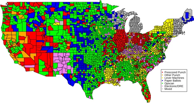
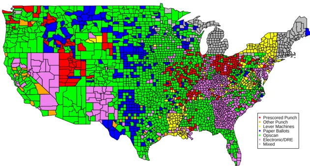
Data
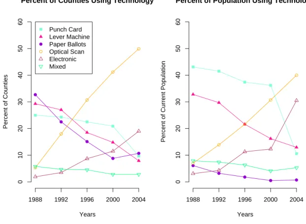
Such counties occur most often in the New England states, where municipal governments administer elections. Paper ballots are most widely used in the Midwestern states; New York and Louisiana are the main states that still use lever machines.
Methods
Difference-in-differences
The distribution of residual voting rates is skewed to the right and a transformation is required to maintain the normality assumption in the least squares specification. However, it is also the case that the distribution of residual voting rates, Yit, has a mass at zero, which is problematic for the log transformation.
Fixed effects models
1{p= 1}is a dummy variable equal to unity if the observation takes place in the second half of the period (that is, for the period 1988-1992, p=1 in 1992); and 1{i∈OS} is a dummy variable with a value equal to unity, indicating that the observation belongs to the treatment group (regions switching to optical scanners). In addition, all observations are weighted by turnout, so that the interpretation of the dependent variable is relative to the total number of votes cast.
Propensity score matching model
This means that the treatment and control outcomes Y1 and Y0 are independent of the treatment assignment, T, dependent on the observed variables, X, and that there is overlap in treatment probabilities. In the context of this particular data, Tit0 are punched card machines, while the processing group is one of the other types of equipment that are considered one by one.10 The Xit vector varies depending on the processing considered, but generally consists of the same covariate, used as controls in fixed-effects regression.
Empirical results
Difference-in-differences estimates
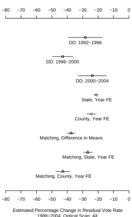
In each of the remaining three periods, counties that switched to punch card optical scanning machines experienced an average decline in residual voting percentage, compared to counties that used punch cards in both elections.
Fixed effects estimates
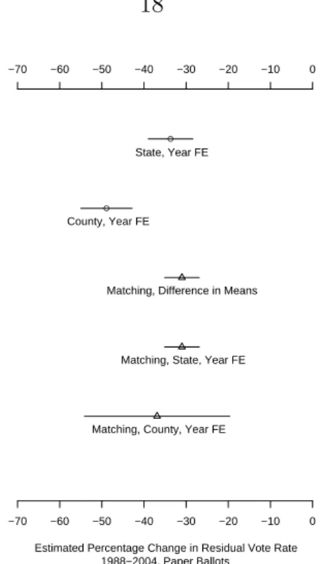
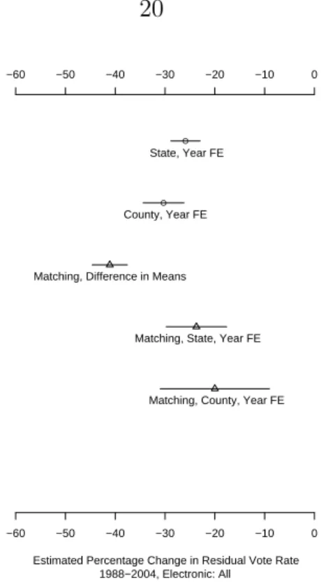
This specification produces the same sequence of equipment types, in terms of reduction in residual voting rates among punched card machines, as the previous model. Although electronic machines and optically scanned ballots do not reduce residual votes to the level estimated for paper ballots, they certainly do much better than punched cards.
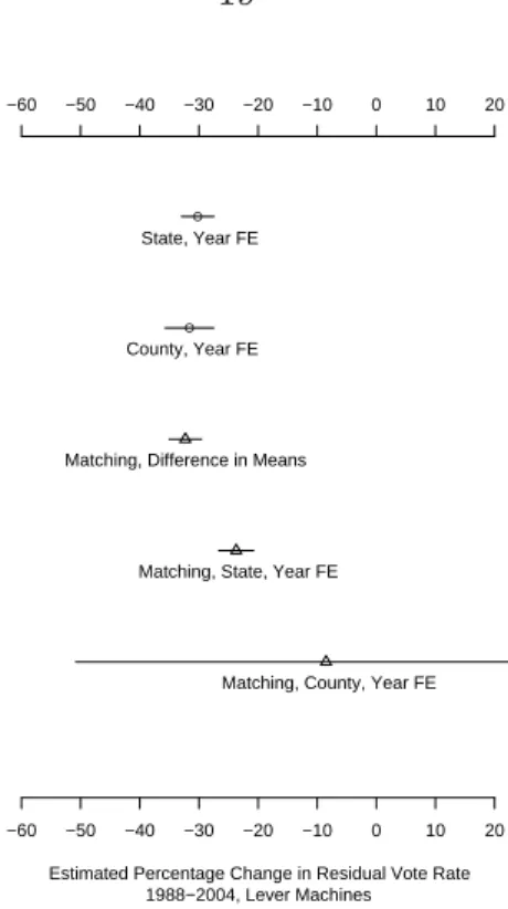
Propensity score matching estimates
Here, paper ballots are the stars, with a 31% reduction in residual voting rates, while optical scanners are a close second with a 28% reduction in rates. Electronic machines produce an estimated 24% reduction in residual voting rates when counties switch from punch cards.
An extension and future research
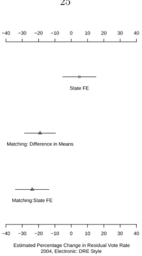
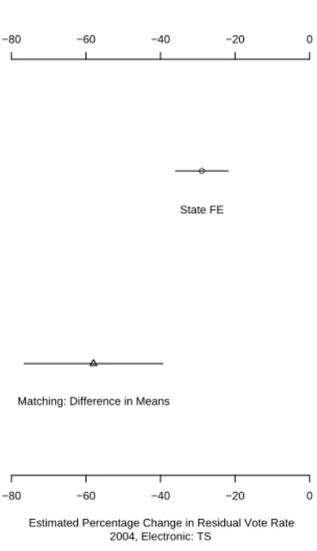
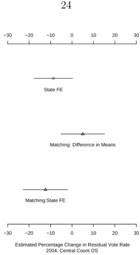
Additionally, by including fixed effects in the parametric analysis, unobserved fixed confounding variables are also controlled. Applying the first fixed-effects model to the data, using the same covariates as in the matching procedure, as well as state and year fixed effects, again yields a new pattern. The analysis of the 2004 data begins with a linear model, which has the transformed residual voting rate as the dependent variable, and the same covariates as in the first fixed effects regression above.
Counties that switch from punch cards to centrally counted optical scanners do not achieve a noticeable improvement in residual vote percentage by either estimate.
Notes
13 This estimate is too small because it does not take into account uncertainty involved in the matching procedure or uncertainty in propensity score estimation. 15To test whether partial or total pooling is appropriate for these data, dummy variables for each period were interacted with the independent variables in the estimated equation, detailed in Section 5.1. The unobservable, fixed temporal effects can be captured by introducing annual fixed effects in the model, the starting point for the specifications in the next section.
The existence preference is an interesting example of causal inference in political science because the treatment—existence status—is initially relatively independent of the other predictors in the model.
Formulating incumbency advantage as a causal inference problem
The rest of the chapter proceeds as follows: Section 3.1 formulates the task advantage as a causal inference problem and discusses in more detail previous attempts to measure it. One way to measure incumbency advantage, then, is to compare the incumbent's vote share in the T −1 election (his last election) and the president's party's vote share in the T election (the open seat election). . Further, while the average of these two quantities, the "slurge," is a better estimate of the task advantage, it is still biased.
The paper continues with the definition of a linear regression model, which reveals the advantage of unbiased measurement of existence.
Data and methods
This formulation compares vote shares in incumbent districts to vote shares in open-seat districts, controlling for the effect of incumbent party and vote share in the previous election. Gelman and Huang (2007) present a hierarchical model of incumbent advantage that allows the advantage to vary among incumbents. An extremely important, but underemphasized, feature of the Gelman-Huang model is the inclusion of a lagged value of the incumbent.
To see this, first consider that one of the best known predictors of current outcomes is generally the past outcome(s).
Classical linear regression approach
To this end, the Gelman-King structural models have vote share, vjt, as a function of position, Ijt, established party, Pjt, and past vote share, vj,t−1.
Propensity score matching approach
A generally acceptable place to start is with a logistic (or probit) regression of the treatment on the covariates in the linear model. The estimated propensity score is a balancing score when we have a consistent estimate of the true propensity score. We know we have a stable estimate of the propensity score when matching on the propensity score balances the raw covariates.
Another advantage of the parametric model applied to the raw data is the repeatability of the results.
Discussion
Notes
Second, I propose a model for properly handling the ordinal nature of the voter identification variable. This article proposes the use of Bayesian shrinkage (or empirical Bayes) estimators to model the ordinal nature of the voter identification variable. However, the sparseness of the data requires some form of parametric or interval restrictions on the variable.
The individual-level data are based on a subset of the questions asked in the 2000 and 2004 Current Population Survey Voter Supplements.
Model
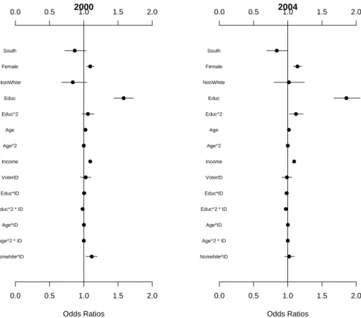
Modeling the impact of voter ID on individuals
Education*VoterID: the interaction between the respondent's reported level of education and the voter identification requirement in the respondent's state;. Education2*VoterID: the interaction between the squared value of Education and the voter identification requirement in the respondent's state;. Age2*VoterID: the interaction between the squared value of Age and the voter identification requirement in the respondent's state; and.
Non-White*VoterID: the interaction between the indicator indicating a reported race other than White and the voter identification requirement in the respondent's state.
Modeling the ordinal nature of voter ID
Specifically for these data, the estimated parameters are a 4 x 1 matrix of group-level intercepts, a 9 x 1 matrix of coefficients on the 9 control variables, and a 1 x 2 matrix of coefficients on the group-level predictor variable for each of the years in the data. This parameter is partially not identified between it and the linear trend in the νj parameters. To correct for this problem, after estimation, the data are “post-processed” to obtain finite population slope parameters based on the regression of αj on Zj.
Given the large scale of the CPS data and the computational intensity of the program, the results presented below are based on only one year, 2000.25 However, previous estimates on the years separately indicate very little difference in the estimates across years.
The impact of voter identification on subgroup turnout
Comparing estimates of the ordinal models
The estimates in figure 4.6 are based on models where the covariates are deprecated and the restricted model is forced to have no intercept term. In the unconstrained model, there is no difference at all between the four coefficients, and the relationship across the regime is non-linear. The Bayesian shrinkage estimator essentially calculates a weighted average between the line and the point corresponding to each ID regime.
In this model, the logistic curve is shifted by an intercept for each identification regime - the difference between this model and the unrestricted model is that these intercepts are drawn to a group of linear trends.
Discussion and future research
It is interesting to note that there is no clear pattern of the effect of the voter identification regime on the likelihood of voting. First, interaction terms between the voter identification variable and the covariates of interest would be included in the model. Because it may also be the case that a voter identification requirement is implemented differently across states, the model will include a random coefficient on voter identification that varies by state.
Then, the model over time would include the voter identification mean for the group and the individual-level identification intercept, in addition to the state group-level mean for the voter identification levels and the state, year, and state*year random intercepts.
Notes
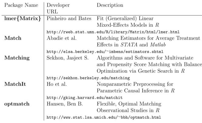
Old Voters, New Voters, and the Personal Vote: Using Redistricting to Measure Incumbency Advantage.” American Journal of Political Science 44:17–34. Designing Observational Studies of Human Populations (with discussion). Journal of the Royal Statistical Society Series A. Assessing the task advantage and its variation, as an example of a before-after study.” Journal of the American Statistical Association (forthcoming).
Causal Inference with General Treatment Regimes: Generalizing the Propensity Score." Journal of the American Statistical Association. The Central Role of the Propensity Score in Observational Studies of Causal Effects." Biometrics. How Does Voting Equipment Affect the Racial Gap in Voided Ballots?” American Journal of Political Science.
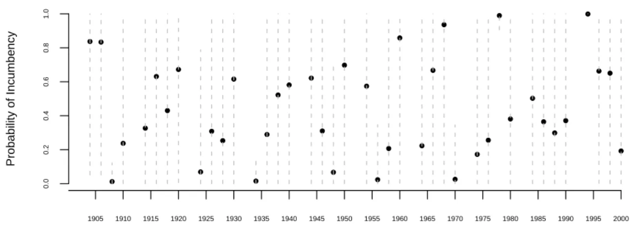
Estimates and 95% Confidence Intervals of Incumbency Advantage, Matched
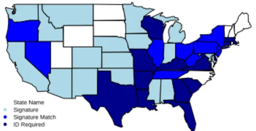
Voter Identification Laws, 2000
Voter Identification Laws, 2004
Marginal Odds of Voting Relative to the Mean Observation
Predicted probability of turnout by ID regime, education level and mi-
Predicted probability of turnout by ID regime, education level and mi-
Point estimates and 95% credible intervals for the three ordinal variable
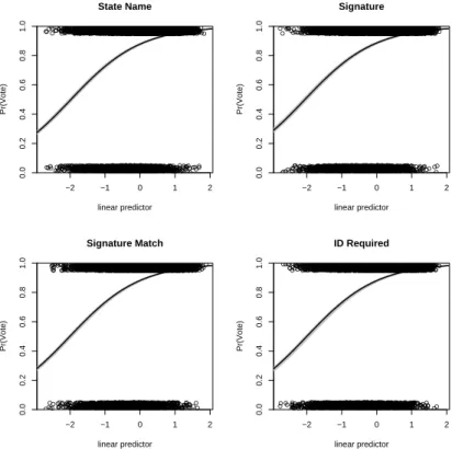
Estimated probability of voting by by ID regime