Habitability Through Time: Photochemistry and Aerosols of Planetary Atmospheres

Introduction

Mars Evolution

Extensive geological evidence, including fluvial features and hydrous minerals, on present-day Mars suggests that a 100–1500 m global equivalent layer (GEL) in meters of liquid surface water once flowed onto the surface of ancient Mars during the late Noachian (> 3.7 Ga ) (Michael H Carr and James W Head, 2003; Clifford and Parker, 2001; Di Achille and Hynek, 2010; Kurokawa et al., 2014). It is currently unknown whether the surface of early Mars was habitable (or habitable).

Exoplanet Observations

Clouds are defined as collections of particles that form in the atmosphere under thermochemical equilibrium (Gao, Wakeford, et al., 2021). Methane clathrates may have formed in the presence of surface ice and serpentine (Lasue et al., 2015).

Crustal Hydration Primed Early Mars with Warm and Habitable

A Comprehensive Photochemical and Climate Model

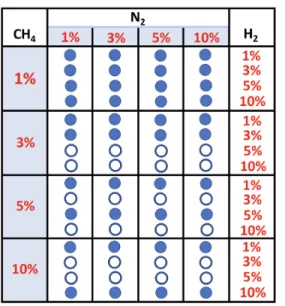
Nair et al., 1994 ) (details in S1), to consider an initial set of five atmospheric pressures and bulk compositions for early Mars. We parametrize sputtering for carbon species (Hu, Kass, et al., 2015) at the upper boundary condition, and we implement crustal hydration (in hot cases) or oxidant.

Figure 2.1: Mars H, C, O chemistry including ground sinks and escape processes.

Crustal Hydration: A Sustained Source of Atmospheric 𝐻

We conclude that lower geological estimates of crustal hydration are not supported by our chemistry and climate model if crustal hydration was indeed the main source of 𝐻2, as low hydrogen fluxes result in surface temperatures too low for surface liquid water. If crustal hydration occurred consistently over long periods of time during the Noachian, we can conclude that the total amount of water lost to the crust is near the upper range of geological estimates.

Figure 2.2: Mixing ratio profiles of 𝐻

Volcanic Fluxes Are Too Low to Sustain Large Ratios of 𝐻

The surface pressure during the warm periods of the Noachian era was probably at least close to 800 mbar, since thinner atmospheres cannot sustain high enough surface temperatures. This pressure constraint agrees with the results of an isotope evolution model (Hu, Kass, et al., 2015), which finds surface pressures of up to 1.5 bar during the Noachian, as well as recent 𝐶 𝑂.

Cool, Dry 𝐶 𝑂

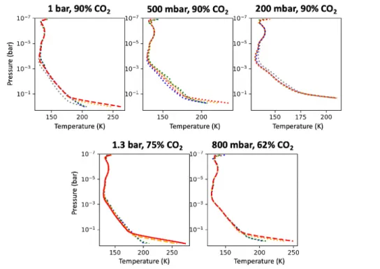
Models are run for the duration of the Noachian era (400 million years), and the resulting profiles after 400 million years are shown. Geologic events could have helped episodically warm a thinning atmosphere (on a short timescale of 105 years), delaying the onset of the CO runaway.

Figure 2.3: Mixing ratio profiles of 𝐻

Implications for Early Mars’ Redox Chemistry

Interestingly, there are both reduced species, including chlorobenzene (Glavin et al., 2013), trichloromethane (Glavin et al., 2013), 𝐻. Hypotheses of perchlorate formation include, for example, not only atmospheric oxidation of chlorine species (Catling et al., 2010) but also formation of brine (Steele et al., 2018) or irradiation of chlorine-containing parent material (Carrier and Kounaves, 2015).

Supporting Information: Materials and Methods

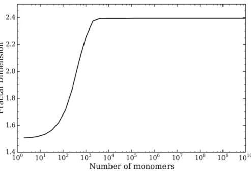
For aggregates, Rannou et al. 1997) treats each monomer as a Mie sphere, and the fractal structure (equation 1) allows a description of the relative position between monomers in the aggregate. These spectroscopic albedo measurements are invaluable for constraining the nature of scattering particles in the atmospheres of these planets (e.g. Barstow et al., 2014).

Figure 2.4: Temperature-pressure profiles computed by REDFOX after iteration with KINETICS

Nitrogen Fixation at Early Mars

Introduction

The astrobiological relevance of lightning-induced nitrogen fixation in the early Earth atmosphere has been considered and motivated by these mechanisms in (Wong, Charnay, et al., 2017). The climate model presented in Wordsworth et al. 2017) produces a global mean surface temperature of >273 K with an atmospheric pressure of less than 2 bar.

Figure 3.1: Summary of the 40 atmospheric compositions we consider. 𝐶 𝐻

Photochemistry due to Lightning at Early Mars

The global mean flash rate is taken into account in the later calculations in this paper, and we derive a value of 5.2𝑥10−17 flash 𝑐𝑚−2𝑠−1 (for details regarding this derivation, refer to Appendix 4), which is comparable to the current - day land speed and early land speed (as determined by the generic LMDZ 3D global climate model; (Wong, Charnay, et al., 2017)). The former can be compared to the NO fluxes on the early Earth, estimated by Wong, Charnay, et al.

Figure 3.2: Annual mean lightning flash rate (log-scale, flash 𝑐𝑚 − 2 𝑠 − 1 ) in a warm, wet, early Mars climate, assuming a global northern ocean for topography at an altitude of -2.54 km

Dissociation of 𝑁

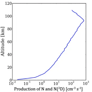
The data from the figure were extrapolated to 6 GeV, assuming the linear log–log relationship shown in the figure, and we assume zero flux for energies greater than 6 GeV. 2dissociation to give N and N(2D) in order to obtain the profiles of production rates 𝑁 and𝑁(2𝐷) induced by SEP events, as shown in Figs.

Photochemical Production and Precipitation of HNOx and HCN

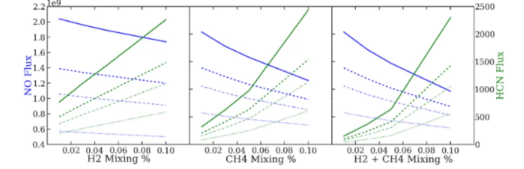
Therefore, the abundance of 𝑁 affects the slope at which reduced gas abundance reduces HO2 production and hence the production rate of 𝐻 𝑁 𝑂. We recall that both 𝑁 and 𝑁(2𝐷) are products of 𝑁 . 2 dissociation via solar events.) This mechanism is summarized in Fig.

Figure 3.4: 𝑁 and 𝑁 ( 2 𝐷 ) production rates (atoms 𝑐𝑚 − 3 𝑠 − 1 ) that result from SEP events as a function of altitude, for an atmospheric composition of 10% 𝑁

Oceanic Concentrations and Astrobiological Implications

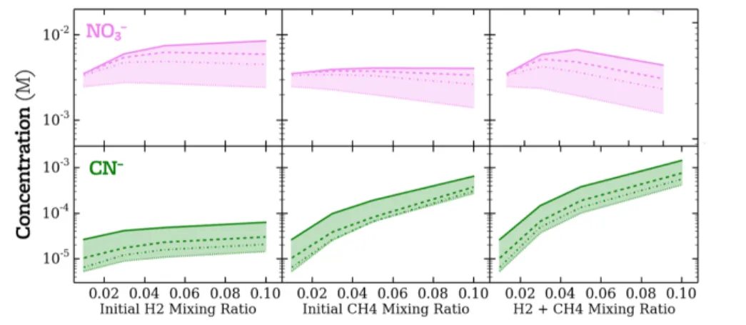
Because hydrothermal vent circulation acts as the sole source of nitrate destruction in early surface waters, concentrations of 0.001−0.01 nitrate are found, which is slightly lower than the expected early Earth concentration of 0.024 M under the same assumption (Wong, Charnay, et al. al., 2017). We find nitrate and cyanide concentration values ​​of 0.1−2𝑛 𝑀 and 0.01−2𝑚 𝑀 (respectively) in a putative northern ocean on early Mars.

Figure 3.9: Concentrations of nitrate (top) and cyanide (bottom) assuming hy- hy-drothermal vent circulation as the only loss mechanism for both species (as in Wong et al., 2017)

Estimating Nitrate Precipitation

In the absence of oceans (e.g. ponds), photodestruction would be more efficient (because they would be shallower), but the deposition area would be reduced. Likewise, if nitrates were involved in biological processes, the death of ocean creatures would also result in sinking and deposition of nitrate-containing compounds on the ocean floor.

Discussion

In future work, we plan to incorporate the feedback mechanism of Hu and Diaz (2019) to determine its impact on early nitrate formation on Mars. Surface lakes and/or ponds are a likely scenario (e.g., Grotzinger et al., 2015); however, investigating steady-state nitrogen concentrations in smaller bodies of water would require some estimate of the fraction of the surface of early Mars covered by this water (which is currently poorly constrained).

Conclusions

HCN hydrolysis is not sensitive to depth and would be approximately homogeneous in any water body (although the rate of destruction would be responsive to water pH (Miyakawa, James Cleaves, and Miller, 2002). Hence, the concentration of HCN in small amounts The water masses would be inversely related to the total amount of surface water over the entire planet.

Appendix 1: KINETICS Model

A critical difference between the two terms is the scale height: in the isothermal case, molecular diffusion drives the system toward diffusive equilibrium as each species follows its own scale height, follow the mass atmospheric scale height,𝐻𝑎.

Appendix 2: GCM Outputs

Appendix 3: Lightning-Induced Fluxes of NO and HCN

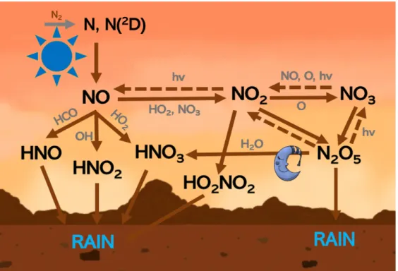
A cartoon of the dominant production and loss mechanisms in the unequal nitrogen cycle is shown in Figure 4.1. Mineral clouds and hydrocarbon particulates in the atmosphere of the hot Jupiter JWST target WASP-43b”.

Explaining Nitrogen Fixation at Paleo-Mars by Investigating

Introduction

2014) considered this mechanism and the subsequent dry deposition of nitric acid gas to estimate the rate of nitrate delivery to the surface. 2021) was the first work to explain the nitrate abundance observed by MSL; however, their mechanism required lightning-induced nitrogen fixation in a warm, wet climate.

Methods

We consider the chemistry of the following species coupled by 152 reactions on a height grid with 1-2 km spacing: 𝑂, 𝑂(1𝐷), 𝑂. We invoke diurnal variations in KINETICS, and the model runs through simulated time to the diurnal cycle of the stratospheric 𝑁 𝑂.

Diurnal Cycle of NOy Reservoirs

We consider a 𝛾 of 0.01 according to Michelangeli et al. 1989), and we calculate the cross section according to an average particle radius of 1.41 microns based on the particle size distributions of Kleinbohl et al. The calculated time-averaged J-profile is plotted in black in Figure 4.2, and the temporal variations are overlaid in various colors.

Heterogeneous Removal of NOy

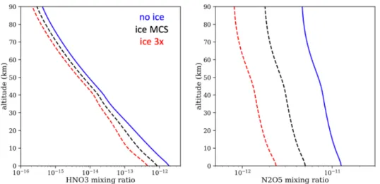
5 on Mars, derived from diurnal variations of NO3, a species sensitive to dayside photolysis. We recognize that ice density varies greatly over time, and as a sensitivity study we consider a third case with ice density increased by a factor of 3; in this case, the steady-state mixing ratios are again reduced by a factor of 2.

Deposition Rate of HNOx on Ice Particles

We consider a case without heterogeneous chemistry (blue; labeled “no ice”) as a control to compare with the scenario considering heterogeneous chemistry with MCS-informed ice data (black). In a third scenario, we accept that the ice number density changes overtime and consider a scenario with tripled ice density.

Figure 4.4: Steady-state mixing ratio of 𝐻 𝑁 𝑂

Interpreting the Formation of MSL-Measured Volatiles

C in the Cumberland, John Klein, and Rocknest samples; 𝑁 𝑂peaks at temperatures above 400 C occur in several samples. We suggest that future work examines the thermal degradation of nitrite- and nitrate-bearing species in Martian soil samples to better constrain the interpretation of the presence or absence of nitrite.

Introduction

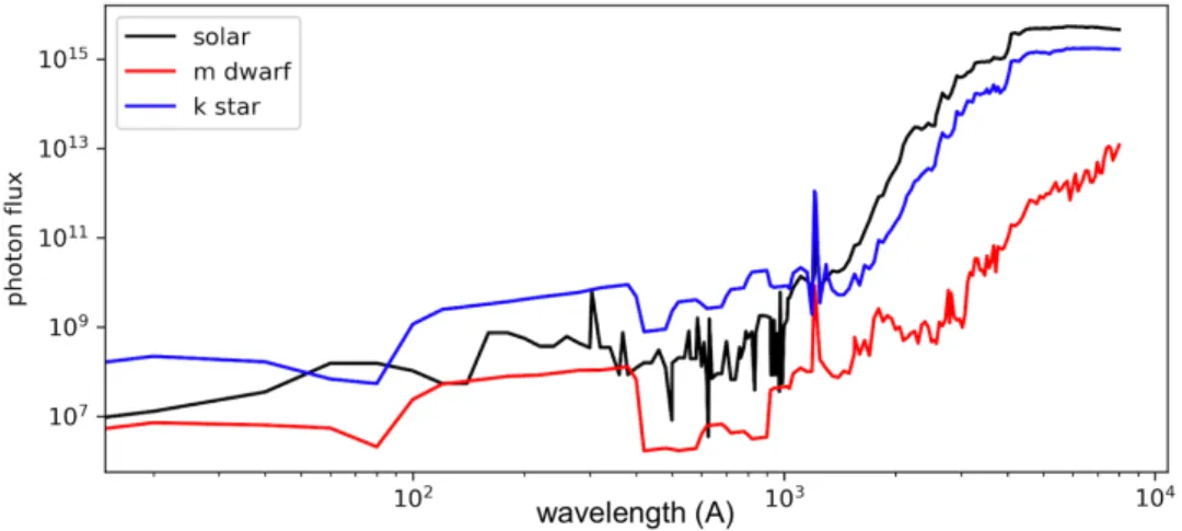
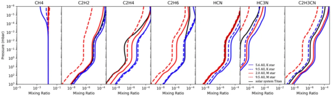
Previous studies have mainly examined the surface climate and atmospheric circulation of Earth-like exoplanets (e.g., Kaspi Showman 2015; Shields et al. Merlis Shneider 2010; Kopparapu et al., 2013), but fewer studies have examined the range of possible conditions on exoplanets. with photochemical hazes, reduced atmospheres and/or different equilibrium temperatures (e.g. Morley et al., 2015; Lora et al. investigate the response of a Titan-like atmosphere to various host stars and find (consistent with the results presented here in section 3 ) that the greater shortwave activity but lower luminosity of M-Dwarfs both result in lower hydrocarbon production Here we investigate the response of a Titan-like atmosphere to a wider range of planetary parameters than previously considered in order to better understand the known atmospheric chemistry to adapt to the conditions of nearby super-Earths: to a warmer temperature, a greater radiation flux, a different stellar type and a different background 𝐻.

Methods

The spectra of K and M stars are obtained from the MUSCLES database (France et al., 2016), and the solar flux is adapted from Gladstone et al. We use Exo-Transmit (Kempton et al., 2016), an open source radiative transfer code that calculates the atmospheric transmission spectrum of transiting exoplanets.

Figure 5.1: Stellar spectra of the Sun (black), an M4.5 host star (red), and a K star (blue), all shown at 1 AU

Results

4 (as on Titan), and the main destruction is again via photolysis to form C2H+H occurs in the upper atmosphere. In the middle atmosphere, most of these inner cycle feedback rates are comparable to the rates on Titan.

Figure 5.2: Response to stellar type and irradiation; all cases are at a Titan-like temperature and 𝑁

GJ 1132b: A Warm 𝐻

Reactions highlighted in blue indicate those with a strong temperature dependence, thus dominating the chemistry in warmer atmospheres.

Discussion

Photochemical nebulae are also common on exoplanets and influence observable observations by acting as gray absorbers and dampening spectral features (e.g., Adams et al., 2019; Kawashima Ikoma, 2019; Zahnle et al., 2016; Marley et al., 2013 ). JWST observations (Batalha et al., 2017), to GJ 1132b, and we find a noise floor of 400 ppm for NIRCAM's G395H instrument (assuming this value varies with wavelength).

Figure 5.14: Mixing ratio profiles of 𝐶 𝐻

Conclusion

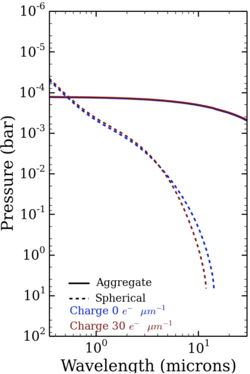
The wavelength dependence of the optical depth of spherical opacity is significant compared to the dependence of aggregate opacity, as shown in Fig. Occasionally, the western zone includes a limb area in the east; see Table 7.3 for a list of zone definitions for each planet.

Aggregate Hazes in Exoplanet Atmospheres

Introduction

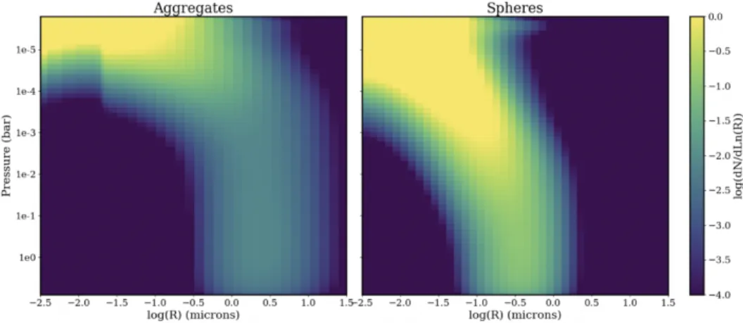
Hazes composed of small (< 0.1 micron) spherical particles, probably of photochemical origin, are generally thought to produce slopes in the optical and NIR regions of the transmission spectra, while condensation clouds with larger spherical particles (1 micron) flatten the spectra at all wavelengths (e.g. Barstow et al. 2017). They concluded that Pluto's photochemical nebulae consist primarily of fractal aggregate particles, although spherical particles may also be present, as inferred from forward scattering observations (Cheng et al. 2017).

Model

The reader is referred to the appendix of Rannou et al. 1997) for more details on this calculation. Recent laboratory work by Horst et al. 2018) showed that the photochemical haze formation rate for a high-metal atmosphere.

Figure 6.1: Variation of aggregate fractal dimension as a function of the number of monomers in the aggregate.

Results

6.8, the optical depth unit occurs 7 scale heights and <1 scale height deeper in the atmosphere for spherical or aggregate nebula. The slope of the unit optical depth level is mostly consistent between the 1 and 10 nm monomer size cases, but the unit.

Figure 6.4: Color map of particle size distributions with respect to atmospheric pressure for aggregate particles (left) and spherical particles (right)

Discussion

The "jump" for the 1 nm monomer cases probably arises from the forced constant mass flux at the top of the atmosphere, which results in a 1 nm monomer haze. The most prominent spectral feature occurs at 6.5 microns and is seen in the spherical case due to the small particle size.

Figure 6.10: Comparison of the pressure level at which unit optical depth occurs when charge is varied from 0 𝑒 − 𝜇𝑚 − 1 (blue) to 30 𝑒 − 𝜇𝑚 − 1 (red) for both aggregate (solid) and spherical (dashed) haze particles

Conclusions

In §7.3, we compare our predicted daily integrated optical albedos with observations of six planets of interest. ATMOSPHERIC CIRCULATION OF HOT JUPITER WASP-43b: COMPARISON OF THREE-DIMENSIONAL MODELS WITH SPECTROPHOTOMETRIC DATA”.

Spatially Resolved Modeling of Optical Albedos for a Sample

Introduction

Vivien Parmentier, Adam P. Showman and Jonathan J. Fortney, 2021; M. T. Roman et al., 2021) use their models to calculate predicted albedos in the Kepler bandpass. Roman et al., 2021, also consider a more extensive grid of planetary models, while also varying cloud compositions, densities and vertical extents.

Figure 7.1: Optical geometric albedo measurements for a sample of hot Jupiters observed in the Kepler bandpass; at these temperatures thermal emission is neg-ligible for planets with cloudy skies and the measured secondary eclipse depth is dominated by re

Methods

For the CARMA simulations in this study, we use the same model setup as in Gao, Thorngren, et al. With the possible exception of Kepler-7b (see §7.4), we expect that such shifts in temperature will not substantially change the pressure of the cloud covers or reduce their horizontal extent for the planets investigated here.

Figure 7.2: Map of the dayside temperatures (in Kelvin) of each planet at 1 mbar, roughly the pressure of unit optical depth in a clear atmosphere in the Kepler bandpass

Results

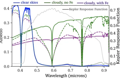
In Figure 7.7 we show the 10×10 grid of albedos in the Kepler bandpass for each planet as a function of 𝑓𝑠𝑒 𝑑. In Figure 7.8 we show the hemisphere-integrated albedos from the full-resolution Virga model from §7.2 rather than the two-zone model discussed in this section.

Figure 7.6: Hemisphere-averaged albedo of K2-107b as a function of wavelength for a clear atmosphere (black) and cloudy atmospheres of varying 𝑓 𝑠𝑒 𝑑 values (green;

Discussion

However, our models for Kepler-7b prefer small cloud particles with a large vertical size; these small particles may have a relatively short lifetime in the hotter substellar region of the dayside atmosphere. For Kepler-7b, whose clouds span much of the Western Hemisphere, it's unclear which of these two competing effects would dominate.

Conclusions

The Atmospheres of the Hot Jupiters Kepler-5b and Kepler-6b Observed During Occultations with Warm Spitzer and Kepler”. An Investigation of Possible Causes of the Holes in the Venus Condensing Cloud Using a Microphysical Cloud Model with a Radiative Dynamical Feedback”.

Conclusion