C H A P T E R 1
Introduction
Market professionals and investors take long and short positions on elementary assets such as stocks, default-free bonds and debt instruments that carry a default risk. There is also a great deal of interest in trading currencies, commodities, and, recently, volatility. Looking from the outside, an observer may think that these trades are done overwhelmingly by buying and selling the asset in question outright, for example by paying “cash” and buying a U.S.-Treasury bond.
This is wrong. It turns out that most of the financial objectives can be reached in a much more convenient fashion by going through a proper swap. There is an important logic behind this and we choose this as the first principle to illustrate in this introductory chapter.
1. A Unique Instrument
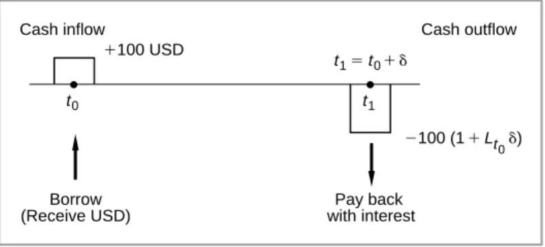
First, we would like to introduce the equivalent of the integer zero, in finance. Remember the property of zero in algebra. Adding (subtracting) zero to any other real number leaves this number the same. There is a unique financial instrument that has the same property with respect to market and credit risk. Consider the cash flow diagram in Figure 1-1. Here, the time is continuous and thet0, t1, t2represent some specific dates. Initially we place ourselves at timet0. The following deal is struck with a bank. At timet1 we borrow USD100, at the going interest rate of time t1, called the Libor and denoted by the symbolLt1. We pay the interest and the principal back at time t2. The loan has no default risk and is for a period ofδunits of time.1 Note that the contract is written at timet0, but starts at the future datet1. Hence this is an example of forward contracts. The actual value ofLt1 will also be determined at the future datet1.
Now, consider the time interval fromt0tot1, expressed ast∈[t0, t1]. At any time during this interval, what can we say about the value of this forward contract initiated att0?
It turns out that this contract will have a value identically equal to zero for allt∈[t0, t1] regardless of what happens in world financial markets. Perceptions of future interest rate
1 Theδis measured in proportion to a year. For example, assuming that a “year” is 360 days and a “month” is always 30 days, a 3-month loan will giveδ=14.
1
t2 t1
t0
Contract initiation
Proceeds received
Interest and Principal paid 1100
2100 2Lt
1d100
FIGURE 1-1
movements may go from zero to infinity, but the value of the contract will still remain zero. In order to prove this assertion, we calculate the value of the contract at timet0. Actually, the value is obvious in one sense. Look at Figure 1-1. No cash changes hand at timet0. So, the value of the contract at timet0must be zero. This may be obvious but let us show it formally.
To value the cash flows in Figure 1-1, we will calculate the timet1-value of the cash flows that will be exchanged at timet2. This can be done by discounting them with the proper discount factor. The best discounting is done using theLt1 itself, although at timet0 the value of this Libor rate is not known. Still, the timet1value of the future cash flows are
P Vt1 = Lt1δ100
(1 +Lt1δ)+ 100
(1 +Lt1δ) (1)
At first sight it seems we would need an estimate of the random variableLt1to obtain a numerical answer from this formula. In fact some market practitioners may suggest using the corresponding forward rate that is observed at timet0in lieu ofLt1, for example. But a closer look suggests a much better alternative. Collecting the terms in the numerator
P Vt1 = (1 +Lt1δ)100
(1 +Lt1δ) (2)
the unknown terms cancel out and we obtain:
P Vt1 = 100 (3)
This looks like a trivial result, but consider what it means. In order to calculate the value of the cash flows shown in Figure 1-1, we don’t need to knowLt1. Regardless of what happens to interest rate expectations and regardless of market volatility, the value of these cash flows, and hence the value of this contract, is always equal to zero for anyt∈[t0, t1]. In other words, the price volatility of this instrument is identically equal to zero.
This means that given any instrument at timet, we can add (or subtract) the Libor loan to it, and the value of the original instrument will not change for allt∈[t0, t1]. We now apply this simple idea to a number of basic operations in financial markets.
1.1. Buying a Default-Free Bond
For many of the operations they need, market practitioners do not “buy” or “sell” bonds. There is a much more convenient way of doing business.
1. A Unique Instrument
3
1100
2100 Pay cash
Receive interest and principal
t2 t1
t0
1rt
0d100
FIGURE 1-2. Buying default-free bond.
The cash flows of buying a default-free coupon bond with par value 100 forward are shown in Figure 1-2. The coupon rate, set at timet0, isrt0. The price is USD100, hence this is a par bond and the maturity date ist2. Note that this implies the following equality:
100 = rt0δ100
(1 +rt0δ)+ 100
(1 +rt0δ) (4)
which is true, because att0, the buyer is paying USD100 for the cash flows shown in Figure 1-2.
Buying (selling) such a bond is inconvenient in many respects. First, one needs cash to do this. Practitioners call this funding, in case the bond is purchased. When the bond is sold short it will generate new cash and this must be managed.2Hence, such outright sales and purchases require inconvenient and costly cash management.
Second, the security in question may be a registered bond, instead of being a bearer bond, whereas the buyer may prefer to stay anonymous.
Third, buying (selling) the bond will affect balance sheets, called books in the industry.
Suppose the practitioner borrows USD100 and buys the bond. Both the asset and the liability sides of the balance sheet are now larger. This may have regulatory implications.3
Finally, by securing the funding, the practitioner is getting a loan. Loans involve credit risk.
The loan counterparty may want to factor a default risk premium into the interest rate.4 Now consider the following operation. The bond in question is a contract. To this con- tract “add” the forward Libor loan that we discussed in the previous section. This is shown in Figure 1-3a. As we already proved, for allt∈[t0, t1], the value of the Libor loan is identically equal to zero. Hence, this operation is similar to adding zero to a risky contract. This addition does not change the market risk characteristics of the original position in any way. On the other hand, as Figure 1-3a and 1-3b show, the resulting cash flows are significantly more convenient than the original bond.
The cash flows require no upfront cash, they do not involve buying a registered security, and the balance sheet is not affected in any way. Yet, the cash flows shown in Figure 1-3 have exactly the same market risk characteristics as the original bond.
Since the cash flows generated by the bond and the Libor loan in Figure 1-3 accomplish the same market risk objectives as the original bond transaction, then why not package them as a separate instrument and market them to clients under a different name? This is an Interest Rate
2 Short selling involves borrowing the bond and then selling it. Hence, there will be a cash management issue.
3 For example, this was an emerging market or corporate bond, the bank would be required to hold additional capital against this purchase.
4 If the Treasury security being purchased is left as collateral, then this credit risk aspect mostly disappears.
(a)
(b)
2100
2100 1100
1100
t2 t1
t0
t0 t1 t2
1Lt
0d100
2Lt
1d100
Received fixed Add vertically
Interest rate swap
Pay floating t2
t1 t0
1st
0 d100
2Lt
1 d100
FIGURE 1-3
Swap (IRS). The party is paying a fixed rate and receiving a floating rate. The counterparty is doing the reverse. IRSs are among the most liquid instruments in financial markets.
1.2. Buying Stocks
Suppose now we change the basic instrument. A market practitioner would like to buy a stockSt at timet0with at1delivery date. We assume that the stock does not pay dividends. Hence, this is, again, a forward purchase. The stock position will be liquidated at timet2. Also, assume that the time-t0perception of the stock market gains or losses is such that the markets are demanding a price
St0 = 100 (5)
for this stock as of timet0. This situation is shown in Figure 1-4a, where theΔSt2is the unknown stock price appreciation or depreciation to be observed at timet2. Note that the original price
1. A Unique Instrument
5
1100
1100 2100
2100 (If Iosses)
t2 t1
t0
t2
t0 t1
DSt
2
DSt
2
2Lt
1d100 (a)
(b)
Equity and commodity swap
Pay if losses DSt
2
Libor
Pay Libor and any losses
Receive any gains (Note the there will be either gains or losses, not both as shown in the graph)
t2 t1
t0
FIGURE 1-4
being 100, the timet2stock price can be written as St2 =St1+ ΔSt2
= 100 + ΔSt2 (6)
Hence the cash flows shown in Figure 1-4a.
It turns out that whatever the purpose of buying such a stock was, this outright purchase suffers from even more inconveniences than in the case of the bond. Just as in the case of the Treasury bond, the purchase requires cash, is a registered transaction with significant tax implications, and immediately affects the balance sheets, which have regulatory implications.
A fourth inconvenience is a very simple one. The purchaser may not be allowed to own such a stock.5Last, but not least, there are regulations preventing highly leveraged stock purchases.
Now, apply the same technique to this transaction. Add the Libor loan to the cash flows shown in Figure 1-4a and obtain the cash flows in Figure 1-4b. As before, the market risk
5 For example, only special foreign institutions are allowed to buy Chinese A-shares that trade in Shanghai.
characteristics of the portfolio are identical to those of the original stock. The resulting cash flows can be marketed jointly as a separate instrument. This is an equity swap and it has none of the inconveniences of the outright purchase. But, because we added a zero to the original cash flows, it has exactly the same market risk characteristics as a stock. In an equity swap, the party is receiving any stock market gains and paying a floating Libor rate plus any stock market losses.6
Note that ifStdenoted the price of any commodity, such as oil, then the same logic would give us a commodity swap.7
1.3. Buying a Defaultable Bond
Consider the bond in Figure 1-1 again, but this time assume that at timet2the issuer can default.
The bond pays the couponct0with
rt0 < ct0 (7)
wherert0is a risk-free rate. The bond sells at par value, USD100 at timet0. The interest and principal are received at timet2 if there is no default. If the bond issuer defaults the investor receives nothing. This means that we are working with a recovery rate of zero. Figure 1-5a shows this characterization.
(a)
(b)
No default
Default 1100
2100
t2 t1
t0
t2
t2 t1
t0
Libor loan
2100 1100
Ct0d100
2Lt
1d100
FIGURE 1-5
6 If stocks decline at the settlement times, the investor will pay the Libor indexed cash flows and the loss in the stock value.
7 To be exact, this commodity should have no other payout or storage costs associated with it, it should not have any convenience yield either. Otherwise the swap structure will change slightly. This is equivalent to assuming no dividend payments and will be discussed in Chapter 3.
1. A Unique Instrument
7
This transaction has, again, several inconveniences. In fact, all the inconveniences mentioned there are still valid. But, in addition, the defaultable bond may not be very liquid.8Also, because it is defaultable, the regulatory agencies will certainly impose a capital charge on these bonds if they are carried on the balance sheet.
A much more convenient instrument is obtained by adding the “zero” to the defaultable bond and forming a new portfolio. Visualized together with a Libor loan, the cash flows of a defaultable bond shown in Figure 1-5a change as shown in Figure 1-5b. But we can go one step further in this case. Assume that at timet0 there is an interest rate swap (IRS) trading actively in the market. Then we can add this interest rate swap to Figure 1-5b and obtain a much clearer picture of the final cash flows. This operation is shown in Figure 1-6. In fact, this last step eliminates the unknown future Libor rates Lti and replaces them with the known swap ratest0.
The resulting cash flows don’t have any of the inconveniences suffered by the defaultable bond purchase. Again, they can be packaged and sold separately as a new instrument. Letting the st0 denote the rate on the corresponding interest rate swap, the instrument requires receipts of a known and constant premiumct0−st0 periodically. Against this a floating (contingent) cash flow is paid. In case of default, the counterparty is compensated by USD100. This is similar to buying and selling default insurance. The instrument is called a credit default swap (CDS).
Since their initiation during the 1990s CDSs have become very liquid instruments and completely changed the trading and hedging of credit risk. The insurance premium, called the CDS spread cdst0, is given by
cdst0=ct0−st0 (8)
This rate is positive since thect0should incorporate a default risk premium, which the default- free bond does not have.9
No default
Default
2100 t2 t1
t0
2Lt
1
2Lt1 1Ct
0
(Assumingd51)
FIGURE 1-6
8 Many corporate bonds do not trade in the secondary market at all.
9 The connection between the CDS rates and the differentialct0−st0is more complicated in real life. Here we are working within a simplified setup.
1.4. First Conclusions
This section discussed examples of the first method of financial engineering. Switching from cash transactions to trading various swaps has many advantages. By combining an instrument with a forward Libor loan contract in a specific way, and then selling the resulting cash flows as separate swap contracts, the financial engineer has succeeded in accomplishing the same objectives much more efficiently and conveniently. The resulting swaps are likely to be more efficient, cost effective and liquid than the underlying instruments. They also have better regulatory and tax implications.
Clearly, one can sell as well as buy such swaps. Also, one can reverse engineer the bond, equity, and the commodities by combining the swap with the Libor deposit. Chapter 5 will generalize this swap engineering. In the next section we discuss another major financial engi- neering principle: the way one can build synthetic instruments.
We now introduce some simple financial engineering strategies. We consider two examples that require finding financial engineering solutions to a daily problem. In each case, solving the problem under consideration requires creating appropriate synthetics. In doing so, legal, institutional, and regulatory issues need to be considered.
The nature of the examples themselves is secondary here. Our main purpose is to bring to the forefront the way of solving problems using financial securities and their derivatives. The chapter does not go into the details of the terminology or of the tools that are used. In fact, some readers may not even be able to follow the discussion fully. There is no harm in this since these will be explained in later chapters.
2. A Money Market Problem
Consider a Japanese bank in search of a 3-month money market loan. The bank would like to borrow U.S. dollars (USD) in Euromarkets and then on-lend them to its customers. This interbank loan will lead to cash flows as shown in Figure 1-7. From the borrower’s angle, USD100 is received at time t0, and then it is paid back with interest 3 months later at time t0+δ. The interest rate is denoted by the symbolLt0and is determined at timet0. The tenor of the loan is 3 months. Therefore
δ= 1
4 (9)
and the interest paid becomesLt0
1
4. The possibility of default is assumed away.10
t15t01 d t1 t0
Borrow (Receive USD)
Cash inflow Cash outflow
Pay back with interest 1100 USD
2100 (11Lt
0d)
FIGURE 1-7. A USD loan.
10 Otherwise at timet0+δthere would be a conditional cash outflow depending on whether or not there is default.
2. A Money Market Problem
9
The money market loan displayed in Figure 1-7 is a fairly liquid instrument. In fact, banks purchase such “funds” in the wholesale interbank markets, and then on-lend them to their customers at a slightly higher rate of interest.
2.1. The Problem
Now, suppose the above-mentioned Japanese bank finds out that this loan is not available due to the lack of appropriate credit lines. The counterparties are unwilling to extend the USD funds.
The question then is: Are there other ways in which such dollar funding can be secured?
The answer is yes. In fact, the bank can use foreign currency markets judiciously to construct exactly the same cash flow diagram as in Figure 1-7 and thus create a synthetic money market loan. The first cash flow is negative and is placed below the time axis because it is a payment by the investor. The subsequent sale of the asset, on the other hand, is a receipt, and hence is represented by a positive cash flow placed above the time axis. The investor may have to pay significant taxes on these capital gains. A relevant question is then: Is it possible to use a strategy that postpones the investment gain to the next tax year? This may seem an innocuous statement, but note that using currency markets and their derivatives will involve a completely different set of financial contracts, players, and institutional setup than the money markets. Yet, the result will be cash flows identical to those in Figure 1-7.
2.2. Solution
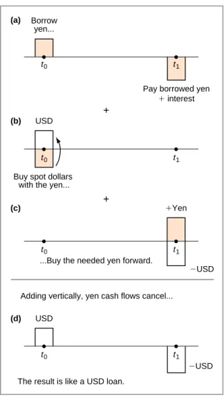
To see how a synthetic loan can be created, consider the following series of operations:
1. The Japanese bank first borrows local funds in yen in the onshore Japanese money markets.
This is shown in Figure 1-8a. The bank receives yen at timet0and will pay yen interest rateLYt0δat timet0+δ.
2. Next, the bank sells these yen in the spot market at the current exchange rateet0to secure USD100. This spot operation is shown in Figure 1-8b.
3. Finally, the bank must eliminate the currency mismatch introduced by these operations.
In order to do this, the Japanese bank buys100(1 +Lt0δ)ft0 yen at the known forward exchange rate ft0, in the forward currency markets. This is the cash flow shown in Figure 1-8c. Here, there is no exchange of funds at timet0. Instead, forward dollars will be exchanged for forward yen att0+δ.
Now comes the critical point. In Figure 1-8, add vertically all the cash flows generated by these operations. The yen cash flows will cancel out at timet0because they are of equal size and different sign. The timet0+δyen cash flows will also cancel out because that is how the size of the forward contract is selected. The bank purchases just enough forward yen to pay back the local yen loan and the associated interest. The cash flows that are left are shown in Figure 1-8d, and these are exactly the same cash flows as in Figure 1-7. Thus, the three operations have created a synthetic USD loan. The existence of the FX-forward played a crucial role in this synthetic.
2.3. Some Implications
There are some subtle but important differences between the actual loan and the synthetic. First, note that from the point of view of Euromarket banks, lending to Japanese banks involves a principal of USD100, and this creates a credit risk. In case of default, the 100 dollars lent may not be repaid. Against this risk, some capital has to be put aside. Depending on the state of money
1 1
t0 t1
Borrow yen...
(a)
USD
Pay borrowed yen 1 interest
Buy spot dollars with the yen...
(b)
2USD ...Buy the needed yen forward.
Adding vertically, yen cash flows cancel...
1Yen (c)
USD
The result is like a USD loan.
2USD (d)
t0 t1
t0 t1
t0 t1
FIGURE 1-8. A synthetic USD loan.
markets and depending on counterparty credit risks, money center banks may adjust their credit lines toward such customers.
On the other hand, in the case of the synthetic dollar loan, the international bank’s exposure to the Japanese bank is in the forward currency market only. Here, there is no principal involved.
If the Japanese bank defaults, the burden of default will be on the domestic banking system in Japan. There is a risk due to the forward currency operation, but it is a counterparty risk and is limited. Thus, the Japanese bank may end up getting the desired funds somewhat easier if a synthetic is used.
There is a second interesting point to the issue of credit risk mentioned earlier. The original money market loan was a Euromarket instrument. Banking operations in Euromarkets are con- sidered offshore operations, taking place essentially outside the jurisdiction of national banking authorities. The local yen loan, on the other hand would be subject to supervision by Japanese authorities, obtained in the onshore market. In case of default, there may be some help from the Japanese Central Bank, unlike a Eurodollar loan where a default may have more severe implications on the lending bank.
3. A Taxation Example
11
The third point has to do with pricing. If the actual and synthetic loans have identical cash flows, their values should also be the same excluding credit risk issues. If there is a value discrepancy the markets will simultaneously sell the expensive one, and buy the cheaper one, realizing a windfall gain. This means that synthetics can also be used in pricing the original instrument.11
Fourth, note that the money market loan and the synthetic can in fact be each other’s hedge.
Finally, in spite of the identical nature of the involved cash flows, the two ways of securing dollar funding happen in completely different markets and involve very different financial contracts.
This means that legal and regulatory differences may be significant.
3. A Taxation Example
Now consider a totally different problem. We create synthetic instruments to restructure taxable gains. The legal environment surrounding taxation is a complex and ever-changing phenomenon, therefore this example should be read only from a financial engineering perspective and not as a tax strategy. Yet the example illustrates the close connection between what a financial engineer does and the legal and regulatory issues that surround this activity.
3.1. The Problem
In taxation of financial gains and losses, there is a concept known as a wash-sale. Suppose that during the year 2007, an investor realizes some financial gains. Normally, these gains are taxable that year. But a variety of financial strategies can possibly be used to postpone taxation to the year after. To prevent such strategies, national tax authorities have a set of rules known as wash-sale and straddle rules. It is important that professionals working for national tax authorities in various countries understand these strategies well and have a good knowledge of financial engineering.
Otherwise some players may rearrange their portfolios, and this may lead to significant losses in tax revenues. From our perspective, we are concerned with the methodology of constructing synthetic instruments.
Suppose that in September 2007, an investor bought an asset at a priceS0= $100. In Decem- ber 2007, this asset is sold atS1= $150. Thus, the investor has realized a capital gain of$50.
These cash flows are shown in Figure 1-9.
Dec. 2007
$50
$100
2$100 invest
Liquidate and realize the capital gains
Jan. 2008 Jan. 2007
Sept. 2007
FIGURE 1-9. An investment liquidated on Dec. 2007.
11 However, the credit risk issues mentioned earlier may introduce a wedge between the prices of the two loans.
One may propose the following solution. This investor is probably holding assets other than theStmentioned earlier. After all, the right way to invest is to have diversifiable portfolios. It is also reasonable to assume that if there were appreciating assets such asSt, there were also assets that lost value during the same period. Denote the price of such an asset byZt. Let the purchase price beZ0. If there were no wash-sale rules, the following strategy could be put together to postpone year 2007 taxes.
Sell theZ-asset on December 2007, at a priceZ1, Z1< Z0, and, the next day, buy the same Ztat a similar price. The sale will result in a loss equal to
Z1−Z0<0 (10)
The subsequent purchase puts this asset back into the portfolio so that the diversified portfolio can be maintained. This way, the losses inZtare recognized and will cancel out some or all of the capital gains earned fromSt. There may be several problems with this strategy, but one is fatal. Tax authorities would call this a wash-sale (i.e., a sale that is being intentionally used to
“wash” the 2007 capital gains) and would disallow the deductions.
3.1.1. Another Strategy
Investors can find a way to sell theZ-asset without having to sell it in the usual way. This can be done by first creating a syntheticZ-asset and then realizing the implicit capital losses using this synthetic, instead of theZ-asset held in the portfolio.
Suppose the investor originally purchased theZ-asset at a priceZ0= $100and that asset is currently trading atZ1= $50, with a paper loss of$50. The investor would like to recognize the loss without directly selling this asset. At the same time, the investor would like to retain the original position in theZ-asset in order to maintain a well-balanced portfolio. How can the loss be realized while maintaining theZ-position and without selling theZt?
The idea is to construct a proper synthetic. Consider the following sequence of operations:
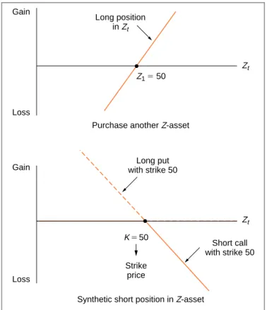
• Buy anotherZ-asset at priceZ1= $50on November 26, 2007.
• Sell an at-the-money call onZwith expiration date December 30, 2007.
• Buy an at-the-money put onZwith the same expiration.
The specifics of call and put options will be discussed in later chapters. For those readers with no background in financial instruments we can add a few words. Briefly, options are instruments that give the purchaser a right. In the case of the call option, it is the right to purchase the underlying asset (here theZ-asset) at a prespecified price (here $50). The put option is the opposite. It is the right to sell the asset at a prespecified price (here $50). When one sells options, on the other hand, the seller has the obligation to deliver or accept delivery of the underlying at a prespecified price.
For our purposes, what is important is that short call and long put are two securities whose expiration payoff, when added, will give the synthetic short position shown in Figure 1-10. By selling the call, the investor has the obligation to deliver theZ-asset at a price of $50 if the call holder demands it. The put, on the other hand, gives the investor the right to sell theZ-asset at
$50 if he or she chooses to do so.
The important point here is this: When the short call and the long put positions shown in Figure 1-10 are added together, the result will be equivalent to a short position on stockZt. In fact, the investor has created a synthetic short position using options.
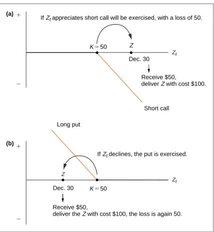
Now consider what happens as time passes. IfZt appreciates by December 30, the call will be exercised. This is shown in Figure 1-11a. The call position will lose money, since the investor has to deliver, at a loss, the originalZ-stock that cost $100. If, on the other hand, theZt
3. A Taxation Example
13
Gain
Loss
Long position inZt
Purchase another Z-asset
Synthetic short position in Z-asset Long put with strike 50
Short call with strike 50 K550
Strike price
Zt Z15 50
Zt Gain
Loss
FIGURE 1-10. Two positions that cancel each other.
decreases, then the put position will enable the investor to sell the originalZ-stock at $50. This time the call will expire worthless.12This situation is shown in Figure 1-11b. Again, there will be a loss of $50. Thus, no matter what happens to the priceZt, either the investor will deliver the originalZ-asset purchased at a price $100, or the put will be exercised and the investor will sell the originalZ-asset at $50. Thus, one way or another, the investor is using the original asset purchased at $100 to close an option position at a loss. This means he or she will lose $50 while keeping the sameZ-position, since the secondZ, purchased at $50, will still be in the portfolio.
The timing issue is important here. For example, according to U.S. tax legislation, wash-sale rules will apply if the investor has acquired or sold a substantially identical property within a 31- day period. According to the strategy outlined here, the secondZis purchased on November 26, while the options expire on December 30. Thus, there are more than 31 days between the two operations.13
3.2. Implications
There are at least three interesting points to our discussion. First, the strategy offered to the investor was risk-free and had zero cost aside from commissions and fees. Whatever happens
12 For technical reasons, suppose both options can be exercised only at expiration. They are of European style.
13 The timing considerations suggest that the strategy will be easier to apply if over-the-counter (OTC) options are used, since the expiration dates of exchange-traded options may occur at specific dates, which may not satisfy the legal timing requirements.
Z
Z
Dec. 30
Short call
IfZtappreciates short call will be exercised, with a loss of 50.
Receive $50,
deliverZ with cost $100.
Zt (a)
K550
Long put
Receive $50,
deliver the Z with cost $100, the loss is again 50.
Dec. 30
Zt (b)
IfZtdeclines, the put is exercised.
K550 1
2 1
2
FIGURE 1-11. The strategy with theZinitially at 50. Two ways to realize loss.
to the new long position in the Z-asset, it will be canceled by the synthetic short position.
This situation is shown in the lower half of Figure 1-10. As this graph shows, the proposed solution has no market risk, but may have counterparty, or operational risks. The second point is that, once again, we have created a synthetic, and then used it in providing a solution to our problem. Finally, the example displays the crucial role legal and regulatory frameworks can play in devising financial strategies. Although this book does not deal with these issues, it is important to understand the crucial role they play at almost every level of financial engineering.
4. Some Caveats for What Is to Follow
A newcomer to financial engineering usually follows instincts that are harmful for good under- standing of the basic methodologies in the field. Hence, before we start, we need to lay out some basic rules of the game that should be remembered throughout the book.
1. This book is written from a market practitioner’s point of view. Investors, pension funds, insurance companies, and governments are clients, and for us they are always on the other side of the deal. In other words, we look at financial engineering from a trader’s, broker’s, and dealer’s angle. The approach is from the manufacturer’s perspective rather than the viewpoint of the user of the financial services. This premise is crucial in understanding some of the logic discussed in later chapters.
5. Trading Volatility
15
2. We adopt the convention that there are two prices for every instrument unless stated otherwise. The agents involved in the deals often quote two-way prices. In economic theory, economic agents face the law of one price. The same good or asset cannot have two prices. If it did, we would then buy at the cheaper price and sell at the higher price.
Yet for a market maker, there are two prices: one price at which the market participant is willing to buy something from you, and another one at which the market participant is willing to sell the same thing to you. Clearly, the two cannot be the same. An automobile dealer will buy a used car at a low price in order to sell it at a higher price. That is how the dealer makes money. The same is true for a market practitioner. A swap dealer will be willing to buy swaps at a low price in order to sell them at a higher price later. In the meantime, the instrument, just like the used car sold to a car dealer, is kept in inventories.
3. It is important to realize that a financial market participant is not an investor and never has “money.” He or she has to secure funding for any purchase and has to place the cash generated by any sale. In this book, almost no financial market operation begins with a pile of cash. The only “cash” is in the investor’s hands, which in this book is on the other side of the transaction.
It is for this reason that market practitioners prefer to work with instruments that have zero-value at the time of initiation. Such instruments would not require funding and are more practical to use.14They also are likely to have more liquidity.
4. The role played by regulators, professional organizations, and the legal profession is much more important for a market professional than for an investor. Although it is far beyond the scope of this book, many financial engineering strategies have been devised for the sole purpose of dealing with them.
Remembering these premises will greatly facilitate the understanding of financial engineering.
5. Trading Volatility
Practitioners or investors can take positions on expectations concerning the price of an asset.
Volatility trading involves positions taken on the volatility of the price. This is an attractive idea, but how does one buy or sell volatility? Answering this question will lead to a third basic methodology in financial engineering. This idea is a bit more complicated, so the argument here will only be an introduction. Chapter 8 will present a more detailed treatment of the methodology.
In order to discuss volatility trading, we need to introduce the notion of convexity gains.
We start with a forward contract. Let us stay within the framework of the previous section and assume thatFt0 is the forward dollar-yen exchange rate.15Suppose at timet0we take a long position in the U.S. dollar as shown in Figure 1-15. The upward sloping line is the so-called payoff function.16 For example, if at timet0+ Δthe forward price becomesFt0+Δ, we can close the position with a gain:
gain=Ft0+Δ−Ft0 (11)
It is important, for the ensuing discussion, that this payoff function be a straight line with a constant slope.
14 Although one could pay bid-ask spreads or commissions during the process.
15 Theet0denotes the spot exchange rate USD/JPY, which is the value of one dollar in terms of Japanese yen at timet0.
16 Depending on at what point the spot exchange rate denoted byeT, ends up at timeT, we either gain or lose from this long position.
Now, suppose there exists another instrument whose payoff depends on theFT. But this time the dependence is nonlinear or convex as shown in Figure 1-12 by the17 convex curve C(Ft). It is important that the curve be smooth, and that the derivative
∂C(Ft)
∂Ft (12)
exist at all points.
Finally suppose this payoff function has the additional property that as time passes the function changes shape. In fact as expiration timeTapproaches, the curve becomes a (piecewise) straight line just like the forward contract payoff. This is shown in Figure 1-13.
5.1. A Volatility Trade
Volatility trades depend on the simultaneous existence of two instruments, one whose value moves linearly as the underlying risk changes, while the other’s value moves according to a convex curve.
First, suppose{Ft1, . . . Ftn}are the forward prices observed successively at times t <
t1, . . . , tn < T as shown in Figure 1-12. Note that these values are selected so that they oscillate aroundFt0.
Ft
4 Ft
2 Ft
0 Ft
1 Ft
3
SlopeD4
SlopeD3 SlopeD1 SlopeD0 SlopeD2
FIGURE 1-12
At time t, t0,t,T
Ft
0
At expiration
FIGURE 1-13
17 Options on the dollar-yen exchange rate will have such a pricing curve. But we will see this later in Chapter 8.
5. Trading Volatility
17
F1 F0
D0
D1
Ignore the movement of the curve, assumed small.
Note that as the curve moves down slope changes
Sell |D02D1| units at F1 Buy |D02D1| units at F0
FIGURE 1-14
Gain at time t, t0,t,T before expiration Expiration gain
Expiration loss
eT eT
Ft
0 Ft
Ft
Slope5 11
FIGURE 1-15
Second, note that at every value ofFti we can get an approximation of the curveC(Ft) using the tangent at that point as shown in Figure 1-12. Clearly, if we know the function C(.), we can then calculate the slope of these tangents. Let the slope of these tangents be denoted byDi.
The third step is the crucial one. We form a portfolio that will eliminate the risk of directional movements in exchange rates. We first buy one unit of theC(Ft)at timet0. Note that we do need cash for doing this since the value att0is nonzero.
0< C(Ft0) (13)
Simultaneously, we sellD0units of the forward contractFt0. Note that the forward sale does not require any upfront cash at timet0.
Finally, as time passes, we recalculate the tangentDiof that period and adjust the forward sale accordingly. For example, if the slope has increased, sellDi−Di−1units more of the
forward contracts. If the slope has decreased coverDi−Di−1units of the forwards.18AsFti oscillates continue with this rebalancing.
We can now calculate the net cash flows associated with this strategy. Consider the oscilla- tions in Figures 1-12 and 1-13,
(Fti−1 =F0)→(Ft1 =F1)→(Fti =F0) (14) withF0< F1. In this setting if the trader follows the algorithm described above, then at every oscillation, the trader will
1. First sellDi–Di−1additional units at the priceF1. 2. Then, buy the same number of units at the price ofF0. For each oscillation the cash flows can be calculated as
gain= (D1−D0)(F1−F0) (15)
SinceF0< F1andD0< D1, this gain is positive as summarized in Figure 1-14. By hedging the original position inC(.)and periodically rebalancing the hedge, the trader has in fact succeeded to monetize the oscillations ofFti(see also Figure 1-15).
5.2. Recap
Look at what the trader has accomplished. By holding the convex instrument and then trading the linear instrument against it, the trader realized positive gains. These gains are bigger, the bigger the oscillations. Also they are bigger, the bigger the changes in the slope termsDi. In fact the trader gains whether the price goes down or up. The gains are proportional to the realized volatility.
Clearly this dynamic strategy has resulted in extracting cash from the volatility of the under- lying forward rateFt. It turns out that one can package such expected volatility gains and sell them to clients. This leads to volatility trading. It is accomplished by using options and, lately, through volatility swaps.
6. Conclusions
This chapter uses some examples in order to display the use of synthetics (or replicating portfo- lios as they are called in formal models). The main objective of this book is to discuss methods that use financial markets, instruments, and financial engineering strategies in solving practi- cal problems concerning pricing, hedging, risk management, balance sheet management, and product structuring. The book does not discuss the details of financial instruments, although for completion, some basics are reviewed when necessary. The book deals even less with issues of corporate finance. We assume some familiarity with financial instruments, markets, and rudi- mentary corporate finance concepts.
Finally, the reader must remember that regulation, taxation, and even the markets themselves are “dynamic” objects that change constantly. Actual application of the techniques must update the parameters mentioned in this book.
18 This means buy back the units.
Suggested Reading
19
Suggested Reading
There are excellent sources for studying financial instruments, their pricing, and the associ- ated modeling. An excellent source for instruments and markets is Hull (2008). For corporate finance, Brealey and Myers (2000) and Ross et al. (2002) are two well-known references.
Bodie and Merton (1999) is highly recommended as background material. Wilmott (2000) is a comprehensive and important source. Duffie (2001) provides the foundation for solid asset pricing theory.
CASE STUDY: Japanese Loans and Forwards
You are given the Reuters news item below. Read it carefully. Then answer the following questions.
1. Show how Japanese banks were able to create the dollar-denominated loans synthetically using cash flow diagrams.
2. How does this behavior of Japanese banks affect the balance sheet of the Western coun- terparties?
3. What are nostro accounts? Why are they needed? Why are the Western banks not willing to hold the yens in their nostro accounts?
4. What do the Western banks gain if they do that?
5. Show, using an “appropriate” formula, that the negative interest rates can be more than compensated by the extra points on the forward rates. (Use the decompositions given in the text.)
NEW YORK, (Reuters) - Japanese banks are increasingly borrowing dollar funds via the foreign exchange markets rather than in the traditional international loan markets, pushing some Japanese interest rates into negative territory, according to bank officials.
The rush to fund in the currency markets has helped create the recent anomaly in short- term interest rates. For the first time in years, yields on Japanese Treasury bills and some bank deposits are negative, in effect requiring the lender of yen to pay the borrower.
Japanese financial institutions are having difficulty getting loans denominated in U.S. dol- lars, experts said. They said international banks are weary of expanding credit lines to Japanese banks, whose balance sheets remain burdened by bad loans.
“The Japanese banks are still having trouble funding in dollars,” said a fixed-income strate- gist at Merrill Lynch & Co.
So Japan’s banks are turning to foreign exchange transactions to obtain dollars. The pre- dominant mechanism for borrowing dollars is through a trade combining a spot and forward in dollar/yen.
Japanese banks typically borrow in yen, which they have no problem getting. With a three- month loan, for instance, the Japanese bank would then sell the yen for dollars in the spot market to, say, a British or American bank. The Japanese bank simultaneously enters into a three-month forward selling the dollars and getting back yen to pay off the yen loan at the stipulated forward rate. In effect, the Japanese bank has obtained a three-month dollar loan.
Under normal circumstances, the dealer providing the transaction to the Japanese bank should not make anything but the bid-offer spread.
But so great has been the demand from Japanese banks that dealers are earning anywhere from seven to 10 basis points from the spot-forward trade.
The problem is that the transaction saddles British and American banks with yen for three months. Normally, international banks would place the yen in deposits with Japanese banks and earn the three-month interest rate.
But most Western banks are already bumping against credit limits for their banks on exposure to troubled Japanese banks. Holding the yen on their own books in what are called NOSTRO accounts requires holding capital against them for regulatory purposes.
So Western banks have been dumping yen holdings at any cost—to the point of driving interest rates on Japanese Treasury bills into negative terms. Also, large western banks such as Barclays Plc and J.P. Morgan are offering negative interest rates on yen deposits—in effect saying no to new yen-denominated deposits.
Case Study
21
Western bankers said they can afford to pay up to hold Japanese Treasury bills—in effect earning negative yield—because their earnings from the spot-forward trade more than compen- sate them for their losses on holding Japanese paper with negative yield.
Japanese six-month T-bills offer a negative yield of around 0.002 percent, dealers said.
Among banks offering a negative interest rate on yen deposits was Barclays Bank Plsc, which offered a negative 0.02 percent interest rate on a three-month deposit.
The Bank of Japan, the central bank, has been encouraging government-lending institu- tions to make dollar loans to Japanese corporations to overcome the problem, said [a market professional]. (Reuters, November 9, 1998).