Precision Measurement of the Neutron Lifetime

Introduction

Lifetime of a free neutron

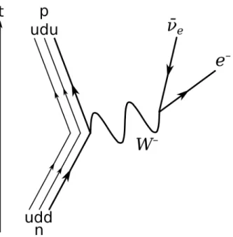
The amplitude of the tree-level process, shown in Figure 1.1, can be calculated using Feynman's rules for weak interactions. This differs from the current global average of free neutron lifetime measurements of 𝜏meas s [1] by '4%.

Figure 1.1: Feynman diagram for the tree-level approximation of the 𝛽 -decay of a free neutron.

Unitarity of the Cabibbo–Kobayashi–Maskawa quark weak mixing

This difference is mostly due to ignoring higher order terms in the 𝛽-neutron decay process. The purpose of the UCN𝜏 experiment is to precisely measure the lifetime of a free neutron.

Big Bang nucleosynthesis and the neutron lifetime

Past measurements of the neutron lifetime

Bottle lifetime experiments
Beam lifetime experiments
Differences between bottle and beam lifetime experiments . 8

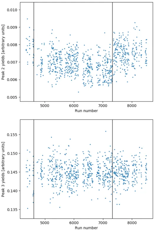
However, the primary detector was only able to sample a fraction of the UCN in the trap at the height of Peak 2. Instability in UCN production during the filling process added uncertainty to the amount of UCN loaded into the trap.

Figure 1.2: A simplified version of how a generic bottle experiment measures the neutron lifetime.

UCN 𝜏 experimental design

Properties of ultra-cold neutrons (UCN)

The defining property of UCN is that they are neutrons that can be stored in material bottles. Given that the maximum energy of UCN is 335 neV, a magnetic field > 5.6 T can completely polarize UCN from their spin.

Overview

The gate valve and the opening in the bottom of the siphon close and the production of UCN stops. The primary detector is lowered to count any UCN remaining in the trap.

Figure 2.1: A CAD drawing of the UCN 𝜏 experimental apparatus. The UCN are produced in the source (left of figure) and diffuse rightward

Production of UCN

This repeated cycle of source temperature causes frost layers to form on the surface of sD2. If most of the sD2 source is in a bad state, then a spontaneous excursion has only a small effect on UCN production.

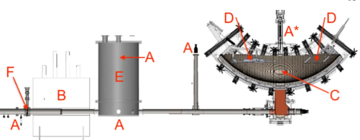
Figure 2.2: A CAD drawing of the LANSCE UCN source [34]. Neutrons are produced by spallation from the W target that is caused by protons that come into the source from the right

Transport of UCN

The first item in the above list is completely outside the control of the UCN𝜏 experiment. The fourth and fifth items in the list can be adjusted if the sD2 resource is reconditioned.

Polarization of UCN

These losses are small enough not to be a problem for the transport of UCN, but would have a significant impact on the service life measured using a material wall trap.

UCN trap

Geometry
Halbach array magnetic walls
Holding field
Putting UCN into the trap

The minimum magnitude of the magnetic field 2 mm above the surface of the trap is 0.81 T. The magnitude of the magnetic field produced by equation 2.5 decreases exponentially as the distance from the surface of the trap increases.

Figure 2.4: A subset of a one-dimensional Halbach array constructed of nine PMs [37]. The direction of the remnant field in each PM is shown with arrows

UCN detectors

Primary detector
Upstream monitors

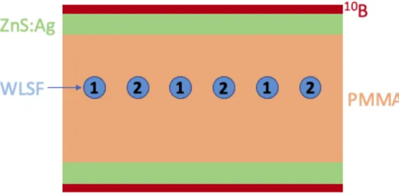
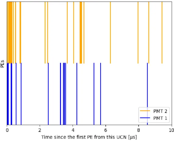
The main feature of the primary detector is the random detection of scintillation light in two PMTs. The primary detector rises above the entire usable volume of the trap while the UCN is stored in the trap.

Figure 2.8: A schematic of the layers of the primary detector. The WLSF alternate which PMT they are connected to, as denoted by the numbering

Removing above-threshold UCN from the trap

Upstream monitors are installed at the bottom of the buffer volume and near the top of the buffer volume. The two detergents remain 43 cm above the bottom of the trap while the UCN is stored in the trap.

Figure 2.10: A CAD drawing of the large cleaner assembly and actuator. The small cleaner has a similar assembly

Upstream buffer volume

However, the buffer size also reduces the number of UCNs loaded into the trap by ~50%. The contributions to the statistical uncertainty of the extracted lifetime from the final number of UCN counted in the trap and the uncertainty of the number of UCN loaded into the trap will be quantified in Section 3.11.

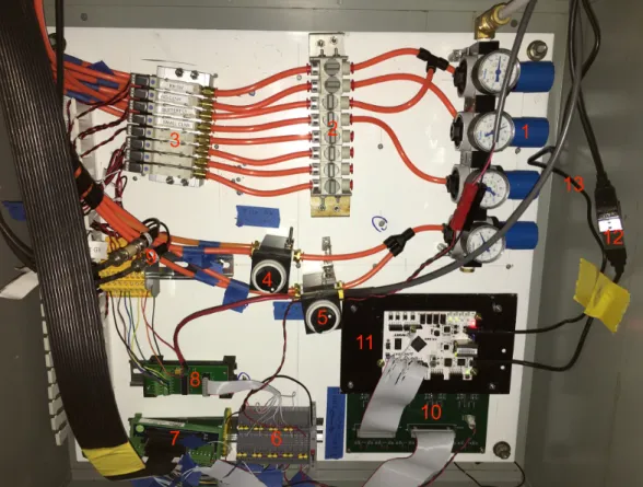
Data acquisition

These marks are caused either by the movement of the components or by the voltage signals that control the components. The rate at which events of any type are recorded is & 300 Hz, so the tags are used to reconstruct component state histories with high accuracy.

Experimental control system

The number of expected CCs was a function of the estimated number of UCN loaded into the trap. The time evolution of the trajectories of UCN in the trap was studied with Monte Carlo simulations [43].

Figure 2.11 shows the hardware that allows the evaluation kit to interface with the rest of the experiment

Extraction of the neutron lifetime

Introduction

An unknown number of UCN is trapped, and the number of UCN in the trap was estimated as𝑁. Fluctuations in the production of UCN resulted in different runs loading different numbers of UCN into the trap at the beginning of each run.

Data structure

Production runs
Background runs
Blinding the data

In the next 100 seconds, the primary detector captured 99.99% of the remaining UCNs in the trap. The primary detector spent 250 s at each of the four heights before the background run ended.

Run selection

Introduction
Fill quality
Blinding bug
Changes in the condition of the primary detector
Conclusion

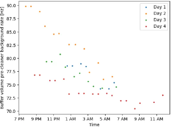
In the lower plot, both the lower and upper monitors were located inside the buffer volume. Occasionally, actions were taken that caused step changes in the behavior of the primary detector.

Figure 3.1: Comparison of UCN monitor rates with and without abnormal pro- pro-duction of UCN

Identification of UCN events in the primary detector

Introduction
Modeling
Simulating UCN events using Monte Carlo simulations
Reconstructing UCN events from PEs
Software dead time
UCN-event-tail interactions
Testing the software-dead-time and UCN-event-tail correc-
Choice of the parameters of the reconstruction algorithm
Conclusion

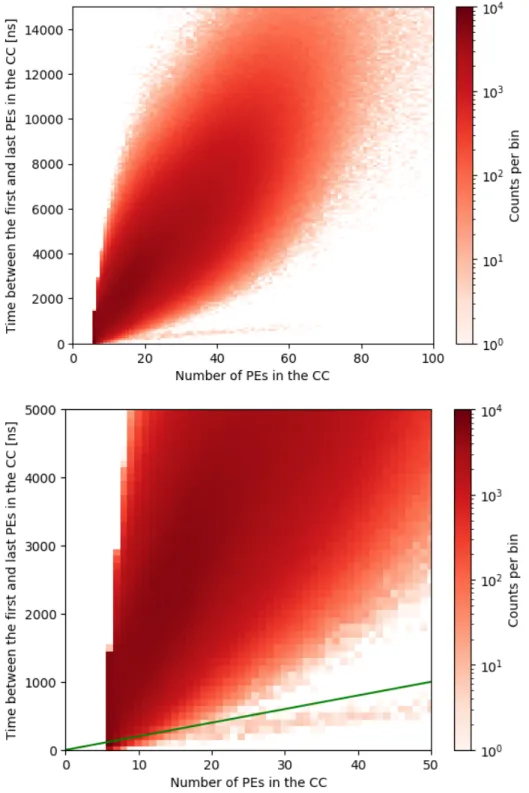
This algorithm estimated the number of PEs in the call window of the current CC that originated from previous UCN events. The potential bias of the extracted lifetime due to errors in the UCN-tail correction of the event will be investigated in Section 3.4.7.

Figure 3.6: PEs generated when one UCN was captured by the primary detector.

Backgrounds

Introduction
Classification of background events
Height-dependent background rates
Time-dependent background rates
Check of the estimation of the background CC rates
Conclusion

No increases in the background CC rates were observed as the primary detector moved between positions. Evidence of this was seen in the background PEs in both PMTs of the primary detector.

Figure 3.15: CCs in the primary detector during the unloading process. The green line in the lower plot represents a CC that consisted of PEs that arrived at a rate of 1 PE per 20 ns

Normalization

Introduction
Normalization monitors
Normalization model
Changes in running conditions
Conclusion

To complete the extraction of a lifetime, an estimate was needed for the number of UCN trapped at the start of the run. Both monitors provided a good measure of the overall number of UCN produced by the source.

Figure 3.21: Changes of the background rate in the buffer volume pre-cleaner as a function of time of day

Likelihood model

Introduction
Step 1: Loading UCN into the trap
Step 2: Holding UCN in the trap
Step 3: Detection efficiency of UCN in the trap
Step 4: Software-dead-time and UCN-event-tail interactions 95
Constructing a likelihood equation
Checking the assumptions using Monte Carlo simulations
Normalization optimization
Conclusion

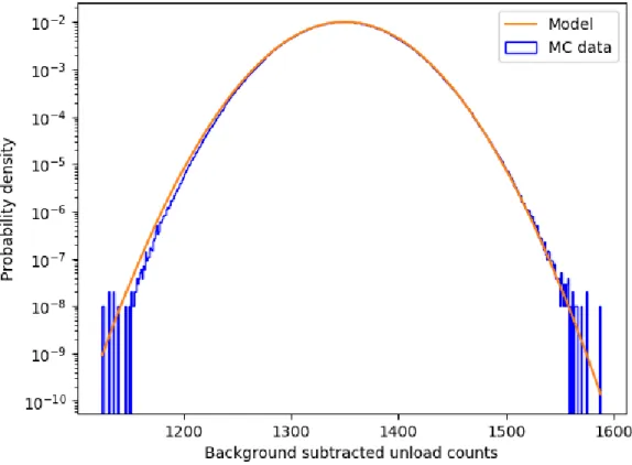
A Monte Carlo value for the number of UCN loaded into the trap is plotted as𝑛 ∼ Integer[Gaussian(𝑁 ,p . 𝑓 𝑁)]. A Monte Carlo value for the number of CCs recorded in the primary detector is plotted as𝑐 ∼Integer[Gauss(𝑠 𝑑 , 𝜎𝑠 . √ 𝑑)].

Figure 3.24 compares the Gaussian distribution in Equation 3.13 to Monte Carlo data generated by sequentially drawing random values following the processes laid out in Sections 3.7.2 through 3.7.6

Holding length

Fixed offsets in holding length
Time evolution of UCN trajectories within the trap

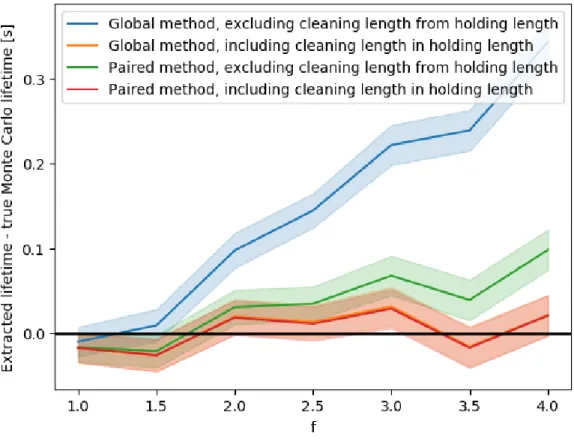
The relatively large number of UCN in Peak 3 outweighed the difference in the Peak 2 component of the arrival time distributions. When the average arrival times of each run are included in the calculation of the Δ𝑡s, the extracted lifetime s was smaller than the actual Monte Carlo lifetime.

Figure 3.26: Bias in the extracted lifetime as a function of the scale of the uncertainty of the normalization estimate 𝜎 𝑁 relative to the ideal case of 𝜎 𝑁 = √

Global analysis

Introduction
Extracting a global lifetime
Statistical bias
Results and conclusion

For a fixed value of 𝜏, the MLE of the normalization parameters was found using the method described in section 3.7.9. If no spectral correction was used in the normalization estimate (see equation 3.6), the global lifetime was 𝜏0.

Figure 3.29: The results of a global lifetime fit of all runs. Top: average yields for each holding length, as well as residuals for each average yield

Paired analysis

Introduction
Bias corrections
Forming run pairs
Extracting a paired lifetime
Statistical bias
Results
Inefficiencies of the paired analysis
Conclusion

First, the paired lifetime extraction used less of the available data because not every run could reasonably fit into a short-long pair. Second, the associated lifetime extraction made less efficient use of the data it did use.

Figure 3.30: Correction to the average of the ratio of yields in a paired lifetime extraction

Conclusion

As discussed in section 5.2, an increase of approximately 10x in the number of UCN loaded into the trap could allow a measurement of neutron lifetimes with a total uncertainty of . Monte Carlo simulations of UCN trajectories in the trap [43] depend on models for the magnetic fields in the trap.

Systematic effects

Introduction

However, there were two cases where UCN in the UCN𝜏 trap interacted with other materials. The corrections that will be developed in Sections 4.2 and 4.3 will be applied on a run-to-run basis before a lifetime is extracted.

Aluminum block interactions

Identifying when the aluminum block fell into the trap
Estimating the effect of the aluminum block on trapped UCN 127

The aluminum block was found and the polyethylene block was placed 6.32 cm above the bottom of the trap. The lifetime of UCN in the trap that did not interact with the aluminum block was not affected.

Figure 4.1: Fraction of total background-subtracted CCs found during Peaks 2 (top) and 3 (bottom) of the unloading process for all of the production runs gathered during the 2017 run cycle

Residual gas interactions

A simple scaling of the lifetime shift by a factor of 𝐴 led to an estimate that the aluminum block reduced the trapped UCN lifetime by between 𝐴×0.11 s=0.08 s and 𝐴×0.28 s=0.21 s. The corrections from Equation 4.4 were applied to batches where the aluminum block was assumed to be trapped.

Figure 4.3: Rate of loss of UCN due to upscattering on residual gasses that remained inside of the trap

Definition of a reconstructed UCN event in the primary detector

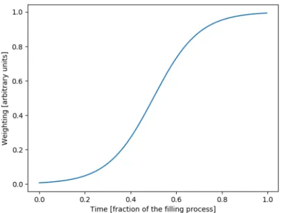
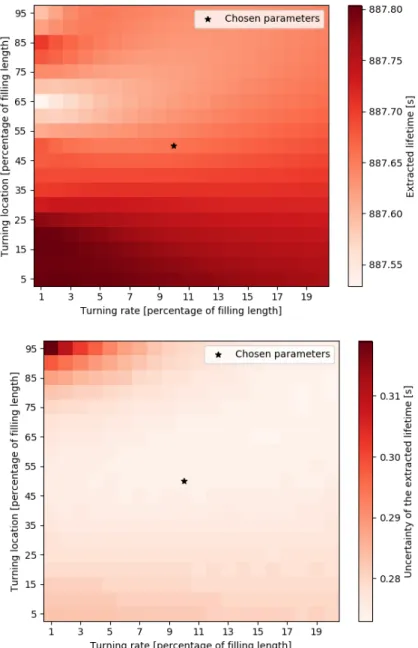
Choice of normalization weighting function

In both plots, the black star represents the spin location and spin rate used in the analyzes of Chapter 3. Earlier turning points gave more weight to the counts recorded earlier in the normalization monitors, even though these counts are mostly uncorrelated with the number of UCN in the trap at the end of the filling process.

Depolarization of trapped UCN

As explained at the beginning of this section, any correction to the extracted lifetime due to loss of depolarized UCN must be strictly nonnegative. The fit shown used the model from equation 4.6, but the fit parameters were extracted using only lifetimes measured with 𝐵 >0.5 mT.

Figure 4.6: Measured lifetimes of UCN in the trap as a function of the magnetic holding field [26]

Insufficient cleaning of quasi-bound UCN

The difference between 𝜅pure and 𝜏 was the estimate of the difference in lifetime extracted due to insufficiently purified nearly bound UCN escaping the trap. Therefore, the systematic uncertainty of the extracted lifetime due to insufficient purification of the quasi-bound UCN was reported as +0.10 s.

Figure 4.7: The results of fitting the no-cleaning data. Top: the 2017 no-cleaning data

Vibrational heating of UCN

Vibrational heating did not cause any UCN to escape the trap during the holding process. As explained at the beginning of this section, any correction to the extracted lifetime due to vibrationally heated UCN escaping the trap must have been strictly non-negative.

Summary of systematic effects

A conservative estimate of 0.08±0.02 s of the correction to the extracted lifetime due to vibrational heating of the UCN was established by summing the two estimates. Therefore, the systematic uncertainty of the extracted lifetime due to vibrational heating of the UCN was reported to be +0.08 s.

Implications of this measurement

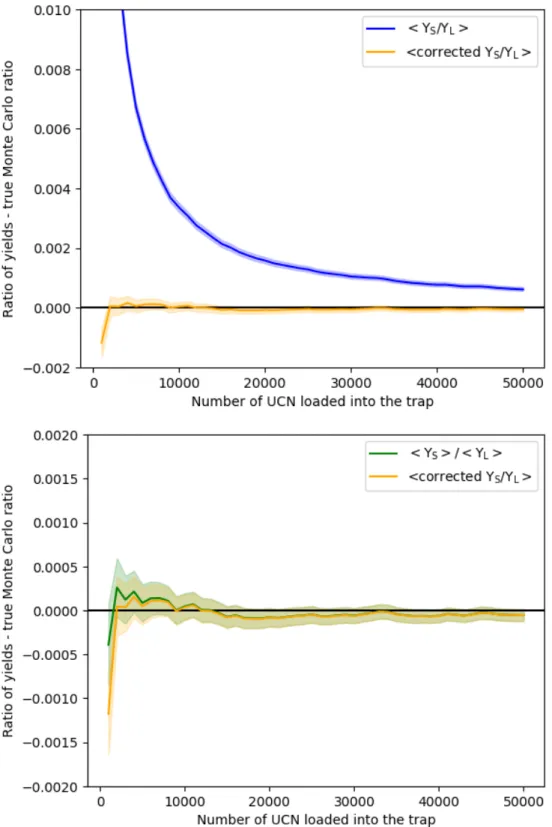
During a typical run from the 2020 run cycle, there was approximately 106UCN in the buffer volume at the end of the fill process. A new method has been realized to use this UCN to reduce the uncertainty of the estimates of the number of UCN loaded into the trap.

Figure 4.8: History of measurements of the neutron lifetime [1, 5–27]. Inset: mod- mod-ern measurements of the neutron lifetime, as well as the current global averages for lifetimes measured using the beam and bottle methods

The future of UCN 𝜏

Introduction

It is expected that after analyzing all data from the UCN𝜏 experiment, a combined lifetime with a total uncertainty of between 0.20 and 0.25 s will be extracted. The next generation version of the UCN𝜏 experiment must have significant upgrades to collect sufficient data to measure the lifetime with an uncertainty of ≤ 0.1 s in a reasonable time.

Increasing the production of UCN

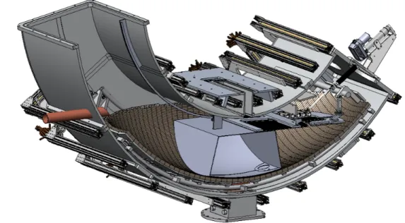
One way to rapidly increase the size of the data set by 10× would be to increase the number of UCN produced by the UCN source. If this proposed next generation UCN source can be built and the 1000× increase in UCN production can be achieved, then measurement of the neutron lifetime to within a total uncertainty of 0.10 s will certainly be achieved.

Figure 5.1: A model of the proposed next-generation UCN source [57]. Three extraction geometries were studied and the “horizontal near-foil” geometry was chosen in order to maximize the production of usable UCN while minimizing engineering constraints

Using the buffer volume as a normalization monitor

Using the UCN remaining in the buffer volume at the end of the priming process as a normalization monitor should significantly reduce the uncertainty of the normalization estimates. Neither of the two normalization monitors installed on the buffer volume during the 2018 run cycle could have counted all of the UCN in the buffer volume.

Improving transport of UCN from the buffer volume to the trap

A new method of transporting UCN from the buffer volume to the trap was proposed. The buffer volume would then be withdrawn from the trap and the cleanup process would begin.

Figure 5.3: A CAD drawing of a proposed buffer volume mechanism to lower UCN into the trap

Next-generation primary detector

The PE velocity in the primary detector with LYSO:Ce dropped to PE velocities close to the background PE velocity within 1𝜇s, which would significantly reduce the number of UCN-to-UCN interactions in the primary detector, even if the maximum rate at which UCN would have been counted increased significantly. Another feature that could be implemented in a next-generation version of the primary detector is pixelization of the active surface.

Figure 5.4: Distributions for times that PEs are observed during a UCN event for primary detectors built with two different scintillating materials [59]

High-precision measurements of magnetic fields in the trap

Magnetic field models that more closely resemble the actual magnetic fields in the trap would improve the accuracy of simulations of UCN trajectories in the trap. Moreover, these magnetic field models can improve simulations that study the possibility that UCN can be depolarized in the trap.

Direct measurement of depolarized UCN

These improvements could further improve the understanding of UCN trajectories in the trap, and could also improve Monte Carlo estimates for the rates at which inadequately cleaned quasi-bonded UCN and vibrationally heated UCN escape from the trap . Instead, an optical camera was mounted above the trap to observe the scintillator at the bottom of the trap and look for flashes of light.

Figure 5.6: A CAD drawing of how an optical camera could be mounted outside of the vacuum jacket [61]

Conclusion

All UCNs are counted exactly 70 seconds after the start of the unloading process, and UCN counting is completely efficient. Monte Carlo simulations are modeled after the simplified version of the UCN experiment described at the beginning of this appendix.