The Role of Transport Phenomena in Whispering Gallery Mode Optical Biosensor Performance

(1)

The Role of Transport Phenomena in Whispering Gallery Mode Optical Biosensor Performance

Thesis by

Jason Gamba

In Partial Fulllment of the Requirements for the Degree of

Doctor of Philosophy

California Institute of Technology Pasadena, California

2012

(Defended June 3, 2011)

(2)

(3)

For Ashley, my wife and friend. Everything changed when I met you.

(4)

Acknowledgements

The fact that a single name appears on the title page of a dissertation can be quite misleading. Neither this document, nor the research behind it, could have been completed without the help of a great number of people.

I would rst like to thank my advisor, Professor Rick Flagan, who has given me the opportunity to work on a project I truly enjoy. I came to him at the end of my third year of graduate school seeking help from the Executive Ocer of Chemical Engineering with nding a new research home on campus. I was looking for a project in a research lab that could support me while I completely rebooted my graduate career, and hoped Professor Flagan could advise me on how to go about my search. After listening to me describe my situation for nearly an hour, he politely asked if I would be interested in hearing about a project available in his own group involving an extraordinary optical biosensor. Within days I was a Flagan Lab member, eager to return to my roots as a chemical engineer by applying the eld's core disciplines to the analysis of what was essentially a physicst's toy. Professor Flagan has taught me a great deal about instrument development and validation, and working in his lab has been an excellent education as a researcher.

I am also very grateful to Professor Andrea Armani, who has been a valuable mentor and friend to me since we began working together in 2008. It was her work as a Clare Boothe Luce Postdoctoral Fellow that began the collaboration between the Flagan, Vahala, and Fraser laboratories at Caltech, of which I have been a part. I was fortunate enough to learn this eld from her, and benet from the extraordinary care and patience she put into developing the procedures she used for her experiments. Even after Professor Armani accepted her faculty position at the University of Southern California, she continued to oer her time to answer my (seemingly endless) questions. I cannot express how helpful this was for a researcher trying to

(5)

learn a eld outside his expertise. Working with her and getting to know her has truly been one of the most rewarding pieces of my graduate career.

I would like to thank Professors Scott Fraser and Mark Davis as well for all of their helpful suggestions and guidance as members of my thesis committee. Of course, my work would not have been possible at all if not for the much-appreciated funding from the Jacobs Institute for Molecular Engineering for Medicine at the California Institute of Technology.

I have also been fortunate to work alongside a wonderful group of researchers in the Flagan/Seinfeld Laboratory. The person who has most aected my own research is Xerxes Lopez-Yglesias. He is a resource of incalculable value to the group, with nearly everyone relying on his broad expertise at one point or another during their tenure. He and I conducted a thorough analysis of the physics involved in sensing a single biomolecule with a whispering gallery mode sensor, debating the value of previous methods and the interpretation of reference texts for hours on end. This intense academic endeavor led us to two main conclusions: (i) that theoretical modeling comes entirely down to how you justify the shortcuts you took in order to preserve your sanity, and (ii) that the selection of Pasadena dining establishments open at 3 am is sadly limited.

Andy Downard is another ne groupmate to whom I am indebted. In addition to being a good friend, Andy was of particular help with my eorts to model the uid ow around sensors. He contributed even more to the daily operations of the lab by generously providing organizational advice and encouraging a multidisciplinary spirit that is too often absent in research environments. Our research group often posed unique challenges, as everyone must quickly develop a broad range of abilities in order to make any progress.

I am grateful, however, to all the members of the Flagan and Seinfeld groups for creating a cooperative and friendly atmosphere, which should never be taken for granted. You all conduct your research (and yourselves) with class in the face of overwhelming pressure to succeed at any cost.

I would also like to thank two outstanding collaborators, Jacob Sendowksi and Naresh Satyan, for their friendship, help, and patience during our work to integrate a tunable laser source of their creation into the nascent sensor apparatus described in the chapters that follow here. Along with the help of other members

(6)

of the Yariv Laboratory in Applied Physics and Electrical Engingeering, especially Scott Steger and Arseny Vasilyev, we began what I hope is a long and productive research partnership for our groups. From the many, many hours I spent working with Jacob and Naresh, I can say that both represent the nest that Caltech has to oer. They are excellent scientists and just truly fun people to be around, both of which only made the grueling frustration of troubleshooting a relatively untested experimental setup that much more pleasant.

Though they get too little credit for the impact they have on student life and graduate research, the various sta at Caltech also deserve a great deal of gratitude. Chemical Engineering administrative assistants like Kathy Bubash, Laura King, Anne Hormann, Marcy Fowler, Martha Hepworth, Karen Baumgartner, and Yvette Grant play a huge role in making sure students have access to their advisors and that the academic machinery continues to run smoothly for everyone. Additionally, a great systems administrator like Suresh Gupta is pivotal in a research environement like Caltech where computation and data storage/transfer are so important. Technical sta, including machinists like Mike Roy, Steve Olsen, and Mike Vondrus as well as glassblowers like Rick Gerhart, are also valuable resources that allow students to push the envelope of their eld by creating new equipment and techniques. It also helps that they are all so friendly, welcoming, and generous with their time. I would like to thank all of these ne Caltech sta members for all of the tasks, large and small, they have helped me with since I started here. I would especially like to thank Mike Roy for teaching me so much about machining and for being such a great friend to me through all of my frustrations.

He is a bright and inquisitive man who perfectly embodies the spirit of Caltech's ingenuity and curiosity.

I also want to point out the contributions that another sta member, Dr. Mike Vicic, has made to my graduate career. He is a truly gifted educator who cares deeply about helping his students learn and remember as much of the mountain of information that the Chemical Engineering curriculum presents to them as possible. I TAed courses administered by Mike three times, and I may have learned more TAing his undergraduate courses than I did during my own undergraduate career. I want to thank him for all of the conversations and guidance he has given me as my friend and unocial mentor. I cannot overstate his value to the Chemistry and Chemical Engineering Division, or to the many students that get the chance to

(7)

interact with him.

One of the most important reasons I chose to come to Caltech for graduate school was the altogether wonderful people that I would get to study with in Chemical Engineering. Though the majority of them graduated (well) before me, I consider myself fortunate to have worked with such a ne group as them.

I am truly lucky to have met and learned from people like Brendan Mack, Nick Brunelli, Yoshie Narui, Chris Alabi, Jim Van Deventer, Chase Beisel, and John McKeen. Thank you all for making Caltech such a wonderful place to be and learn.

These and many other friends enriched my life and helped me make it through the more dicult times in graduate school. Matt Jacob-Mitos and I left Rensselaer Polytechnic Institute as best friends, which is probably why he followed me out to the West Coast for school (albeit to a dierent university). I shudder to put this in writing lest he never let me live it down, but he is one of the brightest people I have ever met and he makes things fun. I owe him a great deal for supporting and continually encouraging my pursuit of a Ph.D. Additionally, Charlotte Mack has been a constant source of fun since I met her many years ago. She is a voice of comfort and inspiration, and her love of life and learning is contagious. I am so very grateful to her and her husband, Brendan, for all of their support through graduate school, my ongoing job search, and life in general. Other brilliant and wonderful friends like Sara Broadhead, Rick Tabor, Chris and Jessica Hansen, and Jackie Kopcsak have all helped me keep a healthy perspective by letting me think and talk about something other than science during all of the fun times we have gotten to spend together. To all of these great friends I give my love, admiration, and thanks.

I want to thank my wonderful family for their extraordinary support. My parents, David and Eileen, have always fostered my curiosity and joy for learning, but their love and encouragement has meant a great deal to me. They have worked so hard to make sure every possible educational opportunity was available to their children, from pre-kindergarten to this day. They have always given me the freedom to pursue my interests, even when that carried me 3000 miles away for graduate school. I am truly fortunate to have such caring and giving parents. I could not have accomplished any of this without their sacrice and love. I want to thank them for all of this, and for raising me a Red Sox fan.

(8)

My entire family has helped me get to this point in my life. I want to thank, in particular, all of my grandparents for being such wonderful examples of how people should treat each other and approach their lives and their work. They are and were passionate individuals, and I love them very much.

Thank you, also, to my brother, David, for always backing me up and helping me to persevere through his encouragement and love. You are the best big brother and friend anybody could have.

Finally, I want to thank my wonderful wife, Ashley. Everything in my life improved when I met you.

There is no way I can thank you enough for the sacrices you have made or the lengths to which you have gone to help me on this (regrettably) long road to graduation. You are an extraordinary woman who volunteered to live the lavish life of a graduate student's wife. I still do not understand what saintly feat I must have accomplished to deserve you, but I am grateful everyday because chance sat me next to you on that airplane. Thank you so very much.

(9)

Abstract

Whispering gallery mode (WGM) optical resonator sensors have emerged as promising tools for label-free detection of biomolecules in solution. These devices have even demonstrated single-molecule limits of detection in complex biological uids. This extraordinary sensitivity makes them ideal for low-concentration analytical and diagnostic measurements, but a great deal of work must be done toward understanding and optimizing their performance before they are capable of reliable quantitative measurents. The present work explores the physical processes behind this extreme sensitivity and how to best take advantage of them for practical applications of this technology.

I begin by examining the nature of the interaction between the intense electromagnetic elds that build up in the optical biosensor and the biomolecules that bind to its surface. This work addresses the need for a coherent and thorough physical model that can be used to predict sensor behavior for a range of experimenal parameters. While this knowledge will prove critical for the development of this technology, it has also shone a light on nonlinear thermo-optical and optical phenomena that these devices are uniquely suited to probing.

The surprisingly rapid transient response of toroidal WGM biosensors despite sub-femtomolar analyte concentrations is also addressed. The development of asymmetric boundary layers around these devices under ow is revealed to enhance the capture rate of proteins from solution compared to the spherical sensors used previously. These lessons will guide the design of ow systems to minimize measurement time and consumption of precious sample, a key factor in any medically relevant assay.

Finally, experimental results suggesting that WGM biosensors could be used to improve the quantitative detection of small-molecule biomarkers in exhaled breath condensate demonstrate how their exceptional sensitivity and transient response can enable the use of this noninvasive method to probe respiratory distress.

(10)

WGM bioensors are unlike any other analytical tool, and the work presented here focuses on answering engineering questions surrounding their performance and potential.

(11)

List of Figures

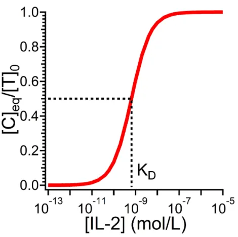
2.1 An equilibrium binding curve for Interleukin-2 with its T Lymphocyte receptor according to Eq. (2.6). Note the sigmoidal shape whose slope approaches zero in the limit of both high and low analyte concentrations. At low [A], the large relative changes in concetration are still too small in terms of total analyte molocules bound. In contrast, the sensor surface is saturated at high [A] and changes in concentration make little aect little change in sensor signal. K_D is marked at6.5×10⁻¹⁰ M. . . 9 2.2 This antibody features four polypeptides: two heavy chain (red) and two light chain (blue).

Note also the "stem-and-arms" conguration, with one FC and two FAB regions. The two complementarity-determining regions (CDRs), where analyte binding occurs, are noted at the end of the twoFAB regions. . . 11 2.3 The non-covalent functioanlization of a biosensor surface via the non-specic adsorption of Pro-

tein G (green) and antibody (black). Exposure to analyte (blue) will lead to binding according to the equilbrium expression in Eqs. (2.1)(2.4). Note the random orientation of the Protein G molecules as well as the fact that not all such molecules are occcupied by an antibody. . . 13

(15)

2.4 Methods for delivering sample to a biosensor. (a) The simple batch method, wherein a droplet of solution is placed onto a planar sensor and diusion delivers sample to the device surface.

(b) The open ow cell with ow injection, featuring a substrate and glass coverslip to form the top and bottom. Surface tension prevents the water from draining, requiring that either the top and bottom surfaces be suciently wettable or the gap suciently small. (c) The microuidic ow cell, a subset of the closed ow cells. These devices are typically made using soft lithography techniques, and their microscale features ensure laminar ow and very little mixing. . . 15 2.5 Field eect transistors (FETs). (a) A generic FET, including the source and drain with conduc-

tion channel between the two. A eld applied using the gate can control the density of charge carriers in the conduction channel and change the current measured at the drain. (b) A nanowire eld eect transistor (FET) sensor. Biomolecules bound to the surface of the nanowire have a localized electric eld that can distort the charge carrier density in the nanowire. Changes in the drain current are used to track how much material has adsorbed to the device. . . 19 2.6 Fluorescence-based biosensor technologies. (a) Total internal reection uorescence (TIRF) is

characterized by the excitation of uorescentlytagged species at a surface by an evanescent eld that decays exponentially and excites only those uorophores near the surface. (b) Sandwich assays feature exposure of an antibody-labeled surface to an analyte solution, followed by exposure to a uorescentlylabeled antibody that binds exclusively to the complex. . . 24 2.7 Surface plasmon resonance (SPR). Here a surface-propagating wave is generated via total in-

ternal reection in a thin gold lm deposited on silica in order to excite a surface plasmon in the metal. Material that adsorbs to the surface shifts the plasmon resonance, which must be compensated for by altering the incident angle of light or the incident wavelength. In this way the surface binding reaction between immobilized targeting species and analyte may be monitored. . . 26

3.1 Whispering gallery mode resonance in the limit of geometric optics. . . 28

(16)

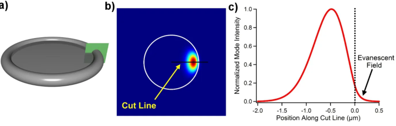
3.2 (a) A toroidal WGM resonator with a cut plane marked in green. (b) An image of the normalized mode intensity along the cut plane in (a) as calculated using the nite element solver COMSOL Multiphysics. (c) A closer look at the normalized mode structure along the cut line in (b) shows the evanescent eld that extends into the water. . . 31 3.3 Flowing PBS buer into the ow cell changes the refractive index of the surrounding medium,

thereby causing a resonance shift according to Eq. (3.10). This is a basic and non-specic sensing method. . . 33 3.4 Transmission spectra depicting a resonance red-shifting a distance∆λin wavelength-space in

response to adsorption of protein to the resonator surface. The minimum fractional transmission, along with the total transmission when no light is coupled into the resonator, may be used to calculate the coupled powerP_D. The value ofQmay also be determined using the observed value ofδλR and Eq. (3.12). . . 34 3.5 The four-step process to fabricate toroidal WGM resonators on (a) a bare silicon wafer with 2

µm of thermal oxide. (b) Photolithography is used to dene a pattern of silica discs through a buered oxide etch process. (c) The chip is exposed to XeF2, an gas that isotropically and selectively etches the silicon from beneath the silica disks. (d) A CO2 laser at 10.6 µm wavelength light is focused normal to the microdisks, melting the edges and leaving microtoroid resonators on silicon pedestals. . . 39 3.6 Three photographs of a single disk during an experiment to use a a KOH etch procedure (10

minute piranha clean followed by a 90 minute exposure to 30 wt% KOH in water) to dene a silica disk followed by reow with a CO2 laser. The anisotropic nature of the KOH etch produces an o-round pedestal, eliminating any chance of a smooth toroid. Note: eld of view in all images is 310µm wide . . . 40

(17)

3.7 Diagrams of experimental reow apparatus. The black arrow indicates the laser source. Plano- convex (PC) lenses made from ZnSe, which does not absorb light at10.6µm like silica optics do, are also shown. The alternative setup proposed in (b) may have the advantages of a cleaner beam prole due to both the spatial lter (pinhole) as well as better control over the beam diameter entering the third PC lens. . . 41 3.8 Coupling of 633 nm light into a 125µm diameter optical ber in water withQ= 2.3×10⁷ . . 43 3.9 Coupling 633 nm light into a microcylindrical WGM resonator. (a) Illumination of the taper

and resonator by a bright eld, and (b) illumination of the system by only the coupled light.

The bright spots in (b) indicate how light is coupled into corkscrew" modes, reaching parts of the ber far from the taper and being scattered. . . 43 3.10 Typical transmission proles illustrating the under-coupled, critically-coupled and over-coupled

regimes. . . 45 3.11 Nonlinear eects observed while coupling into WGM resonators. (a) Asymmetrical transmission

trough for a 150µm microdisk excited with 1310 nm light. (b) Opto-mechanical oscillations as the momentum of propagating light excites mechanical vibration modes in a microtoroidal resonator excited with 1540 nm light. (c) A split resonance peak as backscattering in the cavity can break the degeneracy of counter propagating modes in a microtoroidal resonator excited with 1310 nm light . . . 47 3.12 The WGM sensing experimental apparatus, featuring a tunable laser, tapered optical ber

wavguide, resonator, detector and data capture/processing computer. A function generator is used to sweep linearly through wavelength space so that a transmission spectrum may be used to locate the center of the resonance peak or determine theQof the resonance. . . 50 3.13 The ow cell used in WGM biosensor experiments, shown with a microtoroidal resonator and

tapered optical ber. . . 51

(18)

3.14 Using a tapered optical ber waveguide to couple light into a toroid. (a) A view showing the two in proximity to one another. (b) A low-quality toroidal WGM resonator (Q≈10²) scattering light out of the cavity. . . 51

4.1 Concentration proles for mass transfer to a cylinder in cross section under various ow conditions. Red denotes a normalized concentration of 1, and Blue denotes a normalized concentration of 0. (a) Diusion alone delivers the species to the cylinder isotropically. (b) At low upstream ow velocity, an asymmetric concentration distribution forms, with an extended boundary layer in the wake of the cylinder. (c) At high upstream ow velocity, the boundary layer is thin and the concentration gradient remains asymmetric and is conned to a narrow region around the cylinder. . . 55 4.2 Upstream boundary layer thicknessδ₉₅as a function of inlet ow velocity for spheres of radius

42.5µm(circles) and2.5µm(squares) with predicted scaling laws at high (blue) and low (red) ow velocity limits. The inset graph depicts howδ95 is determined. . . 57 4.3 Time between binding events,τ, for 1 fM analyte concentration solution introduced to toroidal

(circles) and spherical (squares) WGM sensors. (inset) τ recast as a function of sensor Péclet number. . . 58 4.4 The eect of sphere radius on δ₉₅ for varying inlet ow velocities, calculated using the same

model as in Fig. 4.2. . . 59 4.5 Modeled results forτ at a range of concentrations for Interleukin-2 withU = 10⁻² compared

to experimental data published by Armani et al. [1, 2] collected in buer (circle) and bovine blood serum (triangle). . . 60 4.6 Flow cell geometry used in COMSOL Multiphysics simulation of ow around a WGM sensor.

The near plane is a symmetry plane that bisects the cell and the resonator. The sensors are cut out of the cell, and their surfaces feature no-slip ow andC_i = 0 (i.e., instantaneous surface reaction) boundary conditions. . . 64

(19)

4.7 Flow cell boundary conditions used in COMSOL Multiphysics simulations of ow around WGM sensors. (a) Symmetry plane. (b) No-slip" and no ux" conditions. (c) Uniform ow inlet velocity U = U_inlet and inlet concentration C_inlet = 1 fM. (d) Flow outlet at pressure p₀ = 101,325 Pa. . . 65 4.8 The relative surface binding rate to a sphere with Rsphere = 42.5µm and Uinlet = 0.01 m/s

as a function of the surface mesh element size (lmesh=Rsphere/N), calculated with respect to the caseN = 500 (lmesh= 85nm). This quantity converges with increasing N and achieves a relative error of less than 2% for N > 80 (see inset for detail). . . 66 4.9 Solutions for the normalized mode intensity (NMI) of a (a) toroidal and (c) spherical optical

whispering gallery mode resonator. The eective sensing area is determined by where the NMI is greater than 10% of the surface maximum as indicated by dotted lines for (b) a toroid and (d) a sphere. . . 67

5.1 Part of a simulated transmission spectrum that might be observed by measuring the photode- tector output using an oscilloscope while the wavelength is swept at ^dλ_dt = 1.35 nm s⁻¹across a resonance withQ= 10⁸. The full wavelength scan is shown in the inset. The lower horizontal axis is in terms of wavelength detuning fromλ_R while the upper is in terms of time. . . 74 5.2 The normalized mode intensity for λ_R ≈ 680 nm in a (a) spherical (R = 42.5 µm) and (b)

toroidal (r_a= 40µm,r_i= 2.5µm) WGM resonator. . . 78 5.3 (a) Rigorous and (b) modied computation schemes for calculating the WGM sensor response. 89 5.4 The normalized mode prole in a toroidal resonator with major radiusra = 40µmand minor

radiusri= 2.5µmcorresponding to the shown cut line (inset) and the thermal plume resulting from a single-molecule protein heat source exposed to a mode withQ= 10⁸ andPD= 1mW resulting in linear absorption by the molecule. . . 91 5.5 The temperature at the location of the protein (red) and mode peak (blue) as a function of

time where the only heating comes from a protein exhibiting linear absorption bound to the surface of the toroidal sensor withQ= 10⁸,P = 1mW, and ^dλ = 1.35 nm s⁻¹. . . 92

(20)

5.6 The resonance shift due to a single-molecule protein heat source for toroidal resonators (ra = 40µm, r_i= 2.5µm) with P_D = 1mW and ^dλ_dt = 1.35 nm s⁻¹ for varying quality factor. This shift is plotted against a relative time t/τ_res to simplify comparison. The maximum signal is plotted as a function ofQin the inset. . . 92 5.7 The geometry used in COMSOL Multiphysics to solve Eqn. (5.12) for the transient temperature

prole resulting from the excitation of a single-molecule heat source located at what is assumed to be a locally planar interface (blue plane) between a toroidal WGM optical resonator and the water surrounding it. The interior lines are boundaries between subdomains created within the geometry to allow for convenient control over local mesh element size, reducing computation time and memory requirements. . . 95 5.8 Transmission spectrum for a toroid of major radius r_a = 40µm and minor radiusr_i = 5µm

andQ≈10⁷ at wavelength scan rates of (a) ^dλ_dt = 7.6nm/s and (b)−7.6nm/s. The resonator is submerged in water and is being excited using a 765 nm external cavity tunable laser, with a maximum coupled power of 2.6 mW. The dierence in resonance linewidth and transmission minimum is due to thermal distortion of the Lorentzian trough, where λR shifts during the scan when light is absorbed and the system warms. Since this warming results in a red shift ofλ_R, a positive scan rate leads to an articially broad line and a negative scan rate yields an articially narrow line. . . 98

6.1 The structures of arachidonic acid and two of its derivatives most useful as biomarkers of oxidative stress . . . 101 6.2 Typical frequency scan prole shape for external cavity laser (red) and chirp laser (blue). Note

that the ECL has a wider tuning range; however, the OSFL laser has no moving parts so it may attain a far greater range of scan rates. . . 104 6.3 Typical sensor response for a microtoroid resonator in water at 1310 nm exposed to50µL/min

ow of water. The dotted line marks the point at which ow was shut o. . . 107

(21)

6.4 Detection of 100 fM Interleukin-2 in buer using a toroid with Q=2.0×10⁵, a ow rate of 50 µL/min, and a testing wavelength of 1310 nm. The dotted line marks when ow was shut o, and the endpoint resonance shift is marked as∆λ_SS . . . 109 6.5 Detection of 8-isoprostane in buer using a toroid with Q=4.2×10⁵, a ow rate of 50 µL

and a testing wavelength of 1310 nm. The data collection was stitched together to illustrate cumulative resonance shift. First Protein G (red) then polyclonal anti-8ip (blue) were allowed to adsorb. Next, six successively more concentrated 8ip solutions were own into the cell (100 pM, 1 nM, 10 nM, 100 nM, 1µM, and 10 µM). The inset expands this part of the curve for clarity. . . 111 6.6 (a) This sample data for 100µM8ip appears to saturate before ow is turned o (dotted line),

at which point it reaches a new steady state. The endpoint data sought in this measurement is the value of ∆λSS, the true steady state resonance shift. (b) By collecting this endpoint resonance shift and plotting against the concentration of 8ip that elicited that shift, we have a partial dynamic range curve for this system. . . 111

7.1 Modeling results for stagnation point ow around a cylinder with adsorption of IL-2 to its antibody. Upstream owrate is 100µL/min. (a) Dimensionless surface concentration of bound IL-2 at upstream node and downstream nodes as a function of dimensionless time (with respect to characteristic desorption timescale). Flow geometry as depicted in inset, with red lines depicting streamlines and cylinder diameter of 80µm. (b) Dimensionless surface concentration of bound IL-2 as a function of arc length from the upstream node (x= 0m) to the downstream node (x= 1.26×10⁻⁴ m). Each curve corresponds to a singe point in time. . . 117 7.2 This graph shows how the WGM biosensor response appeared for detection of a mixture of

streptavidin protein and streptavidin-coated polystyrene nanoparticles (radiusa= 25nm) with a biotin-functionalized device. This is not actual data. Note the existence of two equilibria: the rst (I) where the surface is populated with bound protein and nanoparticles, and the second (II) where the smaller streptavidin has dissociated and been mostly replaced by nanoparticles. 121

(22)

7.3 This microuidic device diagram demonstrates how the laminar ow in such a device may be used to deposit dierent targeting species (referred to as Antibody 1 and Antibody 2 ) on dierent sensors (labeled 1 and 2 ) simultaneously. For suciently short channels, diusive mixing between the adjacent ow paths will be limited to the small area indicated. . . 127

(23)

List of Tables

5.1 Single-molecule and Single-particle Detection Using∆λR for WGM Optical Biosensors . . . 71 5.2 Summary of Functional Dependencies of Physical Properties . . . 88 5.3 Experimental Parameters for Modeling WGM Biosensing Experiment . . . 98 5.4 Physical Properties of Silica and Water at 298 K and 680 nm . . . 98

6.1 Local Concentrations of 8-isoprostane in the Body [3] . . . 101

(24)

Chapter 1

Introduction

1.1 History and Context

The present work represents the rst foray into the eld of whispering gallery mode sensing, or any biosensing technology, on the part of the Flagan Research Group. During her graduate and post-doctoral research, Dr. Andrea Armani began applying the microtoroidal resonators rst created in the Vahala laboratory in Applied Physics to chemical and biological sensing. When the interpretation of these experiments demanded an expertise in biology and heat transfer, Professors Scott Fraser and Rick Flagan were consulted and a collaboration was born that later produced a publication in the journal Science [1].

I joined the Flagan Group in January 2008 after it became necessary to nd a new laboratory and research project to nish my doctoral work. From January until August I had the privilege to learn from Dr. Armani the methods and theory that she developed in her work with microtoroidal whispering gallery mode (WGM) biosensors. She ordered components and oversaw my construction of a new experimental setup to mimic the one she used in the Vahala laboratory and another being built concurrently in the Fraser laboratory. I was trained on the ner points of pulling tapered optical ber waveguides, using aCO2laser to reow silica disks into toroids, coupling light into the toroidal cavity, and, nally, performing a sensing experiment in an acqueous environment.

My intentions when I joined the Flagan Group were to bring a chemical engineer's perspective to the evaluation of the nascent WGM biosensor. The single-molecule sensitivity observed by Dr. Armani begged

(25)

more questions than it answeredespecially when it comes to evaluating the future of this technology. How the sensitivity scales with molecular size, laser scanning rate, wavelength, and uid ow rate all matter when optimizing operating conditions. Additionally, it becomes important to determine the advantages and disadvantages of single-molecule sensitivity when a slightly worse sensitivity is still orders of magnitude better than alternative technologies but does not require as much eort for data analysis.

There was doubt expressed concerning the results in the Science paper beginning shortly after its publication, but it did not develop until a recent publication attempted to reconcile the proposed physical model with current models and to address the extraordinary sensitivity. While no evidence has been presented to doubt the validity of the experimental observations, it became clear that fundamental questions remain unanswered concerning the basic interactions between the electromagnetic elds in the resonator and the biomolecules that adsorb to the surface. It was at this point that I began the work in Chapter 4 concerning a full description of the heat transfer that would be a part of the thermo-optical model of WGM sensor performance. My progress was limited by my lack of familiarirty with the theory concerning electomagnetic elds and waves, and I began collaborating with labmate Xerxes Lopez-Yglesias to form a complete model that would allow us to compare Dr. Armani's results to a more thorough theoretical prediction. The problem turned out to be monstrously complex, and so we instead crafted a roadmap to guide future work that itself provided new insight and corrected mistakes propagated in the previous literature.

I continued running WGM biosensing experiments in an eort to demonstrate how these devices could be used to detect pollen fragments that play a role in asthma exacerbation. Unfortunately that project was sidetracked by poor luck; the New Focus Velocity^TMtunable laser source at the heart of the WGM sensing experiment was broken when we received it and, after being returned to us 6 months later, immediately began to degrade in performance and cause artifacts in the data until it was no longer functional. I turned my focus back to modeling the eects of mass transport on WGM biosensor performance, yielding the work in Chapter 5. This work has only begun addressing the many interesting problems involved when extraordinarily intense light is present during an equilibrium surface reaction.

The present work is intended to serve as a foundation on which future research into the many physical

(26)

processes involved in WGM biosensing may build. My original research plans involved expanding the applications for these devices; however, that changed when when I saw opportunities to improve our understanding of WGM biosensors behavior and have a greater impact on the eld by modeling the transport phenomena that, until now, have received little attention. This work ultimately addresses fundamental questions that would otherwise hinder the evolution of this technology toward a viable instrument, and, in doing so, presents methods that may be used to address some of the remaining challenges.

1.2 Thesis Structure

This thesis is arranged to serve as a primer for those who hope to conduct WGM biosensing experiments in the future. Chapter 2 introduces the eld of biosensors and, more generally, the specic molecular recognition events that go into a successful bioassay. I describe sample preparation and useful surface chemistries, and review some of the current label-free biosensing technologies that one might encounter in the literature.

Chapter 3 continues the introduction by focusing on WGM resontors and sensors. Topics in this chapter include fabricating, characterizing, comparing, and modeling these devices.

Chapter 4 explores the signicance of uid ow and mass transfer on the transient data observed using a variety of WGM biosensor geometries. Specically, that work explores how the asymmetric concentration boundary layers that form around the sensor in the WGM biosensor ow cell enhance the transient early portion of the transient response, giving rise to the surprisingly fast binding time observed by Dr. Armani that had, until now, puzzled those who work with these devices. Chapter 5 includes the work done in collaboration with Xerxes Lopez-Yglesias to model the relevant physical processes involved in WGM sensing of single molecules. As mentioned above, it is a guide for those interested in modeling the entire, complicated process including nonlinear thermal and optical eects. In Chapter 6, I describe experimental work that seeks to advance WGM biosensors toward medically relevant applications for which they pose a unique solution.

In particular, I detect a small molecule biomarker for oxidative stress in the respiratory system that can be found at low concentrations in exhaled breath condensate. Establishing that the WGM biosensor outperforms

(27)

other analytical techniques for this measurement may make help expand into lower-concentration regimes the working library of biomarkers available for use in diagnostic medicine.

Finally, Chapter 7 concludes this document by reviewing ndings and discussing the many interesting places this research may lead. I truly hope that those who read this document see the promise in this type of biosensor technology, but also realize that a great deal of work must be done before it can be used in practical analytical or diagnostic applications.

(28)

Chapter 2

Biosensors

2.1 Overview

The recent trend toward integrated and automated instruments based on bioassays has had an extraordinary impact on the speed and eciency with which analytical and diagnostic measurements can be made. Bioas- says are methods by which one may determine the absolute or relative concentration of a specic biomolecule in a sample; the target molecule is called the analyte. The researcher attempting to measure how well a new drug works, the medical laboratory technician testing a patient's blood for disease, and even the biology graduate student manipulating genes in an eort to understand a fundamental cellular function relies on a bioassay to get his or her answer.

Each bioassay is characterized by a method that translates the quantity of analyte present in the sample into a measureable signal. Any device that can uses biomolecular interactions at its surface to report this signal while rejecting unintended, nonspecic signal is called a biosensor. It is indeed discouraging to observe in the literature the variety of meanings given to these words; the denitions chosen here are based on those used by the International Union of Pure and Applied Chemistry (IUPAC) [4].

My work focuses on one variety of biosensorthe whispering gallery mode (WGM) optical resonator. I describe the details of this type of device, as well as its fabrication, in Chapter 3. WGM optical resonators have only been used for biosensing applications for less than a decade [5, 6] and the performance and limitations of the technology are still being characterized and debated. It is clear already, however, that

(29)

these devices exhibit extraordinary sensitivity and show great promise as a future analytical or diagnostic instrument. This process by which a technology is built into an integrated instrument is slow and laborious, however, and requires an understanding of the many factors that contribute to its performance. The results presented in Chapters 4 through 6 aim to advance this understanding and, hopefully, inform the development of an instrument.

This chapter describes the features common to all biosensors and introduces a range of example technologies: (i) a method for detecting biomolecules, (ii) a method for ensuring only specic detection, and (iii) a method for introducing sample. With these in mind, I introduce the biosensor technologies in use today and explore their advantages and disadvantages. Finally, I discuss what researchers in the WGM biosensing eld can learn from these alternatives, and what challenges must be addressed in the ongoing eort to develop a WGM biosensor instrument.

2.2 Specic Detection

A key function of a biosensor is the ability to either ignore signal from molecules other than the analyte or to actively stie all interactions other than those with the species of interest. Though the latter is the far easier option in nearly all cases, it would be misleading to suggest that either option is, by any means, simple. To reject all interactions other than those with the analyte, the surface of the sensor may be functionalized with a targeting species that will interact only with the analyte.

The interaction between two species that have a particularly high and exclusive anity for one another is called specic binding, and it is due to a variety of factors. It is often depicted as a simple geometric match, with one molecule possessing a "binding pocket" shaped perfectly for its ligand. While this is often the case, a more complete model must take into account the balance between attractive and repulsive forces as well as the overall energy of the bound and unbound systems. The more common type of interaction is called nonspecic binding, and it implies only that there is an anity between two species.

The best example of nonspecic binding is highlighted by the work of Leo Vroman, who spent much of

(30)

his career as a hematologist studying how proteins in blood plasma adsorb to surfaces. There is no specic interaction between a protein, such as brinogen, and a surface like glass, but it adorbs to a microscope slide nevertheless because the protein is not rigid. Its tertiary structure bends and stretches, sampling a range of conformations. The hydrophobic residues that are typically hidden in the center of the protein to limit their exposure to the polar water molecules in the solvent can induce a restructuring with two eects: (i) these hydrophobic residues can be pressed against the surface (typically less polar than water) to further decrease the strength of their interaction with the solvent and (ii) more of the hydrophilic residues can interact with water due to the higher surface area-to-volume ratio of the pancake-like bound protein [7].

Any generic interaction, including a pure Coulombic one that might draw all positively or all negatively charged species to the sensor surface, can be considered non-specic. Rejecting all signals due to the many possible nonspecic binding methods is, indeed, a challenge.

A popular method to reject this type of undesired adsorption in favor of specic interactions is to simply coat the sensor surface with the targeting species, such that there is no remaining space for other species to occupy. Attaining such high surface coverage is very dicult because of steric eects. An alternative approach is to ll the space between targeting species molecules with a material that actively rejects nonspecic adsorption, e.g., polyethylene glycol (PEG) [8, 9]. It is believed that the high density of hydroxyl groups in PEG produce a structured and stable water layer that would be disrupted (a signicant enthalpic penalty) by nonspecic adsorption by other species. A variety of surface treatments have been developed toward a similar purpose [10]. Several have even been incorporated into a molecular architecture that includes the targeting agent [11, 12, 13].

Reversible binding of the analyte to the targeting species can be described using a simple Langmuir kinetic model where[A]is the concentration of analyte,[T]is the surface concentration of unbound targeting species, [C] is the surface concentration of the bound complex, and[T]0 is the total concentration fo the targeting species. The adsorption/desorption reaction

A + TC

(31)

proceeds at a forward (adsorption) rate,

rate_ads=k_ads[A][T], (2.1)

and a reverse (desorption) rate,

ratedes=kdes[C]. (2.2)

The rate of change of the free analyte concentration is

d[A]

dt =−kads[A][T] +k_des[C]. (2.3)

At equilibrium, ^d[A]_dt = 0, and

kdes

k_ads =KD= [A][T]

[C] (2.4)

is the equilibrium dissociation constant. The total concentration of tageting sites [T] is conserves, so the concentration of available sites is [T] = [T]0−[C]. Therefore, the bound analyte concentration varies with time as

d[C]

dt =kads[A]([T]0−[C])−kdes[C], (2.5) and asymptotically approaches the steady-state (or equilibrium") value of

[C]eq= [A][T]0

K_D+ [A]. (2.6)

It is simple to show that half of all binding sites are occupied when [A]=KD. The sensor response as a function of[A]enables measurement ofKD as illustrated in Figure 2.1 for the protein Interleukin-2 [14].

It is worth pointing out that interaction between an analyte and its targeting species can be a delicate function of experimental conditions. Not only is the anity (K_D) a function of temperature due to the eect of thermal uctations (or lack thereof) on the probability that two species will be able to bind to one

(32)

Figure 2.1: An equilibrium binding curve for Interleukin-2 with its T Lymphocyte receptor according to Eq. (2.6). Note the sigmoidal shape whose slope approaches zero in the limit of both high and low analyte concentrations. At low [A], the large relative changes in concetration are still too small in terms of total analyte molocules bound. In contrast, the sensor surface is saturated at high [A] and changes in concentration make little aect little change in sensor signal. KD is marked at 6.5×10⁻¹⁰ M.

another, but the very structure of the species involved often changes with pH, salt concentration, ambient light, and temperature. One should always keep in mind when using biomolecules that they (for the most part) did not evolve for the sole purpose of a bioassay in a research laboratory. They can be unstable, ckle, and uncooperative when it comes to varying experimental conditions.

Targeting Species

The challenge of nding a species to serve as the targeting agent on a biosensor surface has, thankfully, been addressed by the slow and methodical process of evolution. Biomolecules comprise a vast array of species that exist within organisms, including nucleic acids, proteins, and fatty acids. Each species serves a

(33)

particular purpose in an organism, and must interact with other biomolecules in order to accomplish it. The problem of nding a targeting species for a given analyte often comes down to nding the complimentary molecule that evolved to interact with it. Consider nucleic acids, which consist of two chains of repeated units called nucleotides. Deoxyribonucleic acids (DNAs) feature the well-known double helix structure in which the two opposing chains form bonds with one another much like the steps in a ladder. There are only four varieties of nucleotides in DNA; the double helix cannot form unless each nucleotide in the sequence is paired with its one complimentary nucleotide on the the opposing strand. Immobilizing a short, single strand of DNA on the surface of the sensor allows only complimentary strands to bind on the device surface with appreciable stability [15]. Much like with a long zipper with only a single tooth unzipped, however, a long target strand could possibly bind a slightly mismatched sequence because the energetic favorability of the bonds that form outweighs the entropic penalty of immobilization.

The principle of complimentary nucleic acid sequences extends beyond this simple example, though.

Aptamers can be used where biology has not produced a tailor-made targeting species, even though it provides the architecture to do so. These oligonucleotides are designed with a sequence that will envelop and bind to a particular species [16, 17, 18]. Methods have been established by which a researcher can evolve an aptamer for an arbitrary analyte [19]. Their capability to encode adaptable molecular recognition has even made them appealing tools for gene-regulation platforms [20]. Though the binding anitiy of aptamers for their analytes varies greatly [21], they can attainK_D values as low as 1 nM.

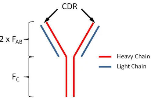
Perhaps the most popular targeting species for biosensing applications is the antibody. These proteins, also called immunoglobulins, are a part of the body's immune response and featureKDvalues of0.1−100nM for their antigens. They consist of four polypeptide chainstwo heavy chains and two light chainsconnected to one another via sulde bonds (see Fig. 2.2). As with all proteins, the variations among antibodies that allow analyte-specic interactions are due to the order in which the 20 available amino acids are arranged, and the tertiary structure to which this sequence leads. Figure 2.2 shows the coarse anatomy of an antibody, which features a stem (the "F_C" region) and two arms (the "F_AB" regions). At the end of eachF_AB region is a complementarity-determining region (CDR) that accounts for the source of variation from one antibody

(34)

Figure 2.2: This antibody features four polypeptides: two heavy chain (red) and two light chain (blue).

Note also the "stem-and-arms" conguration, with oneF_Cand twoF_ABregions. The two complementarity- determining regions (CDRs), where analyte binding occurs, are noted at the end of the twoF_AB regions.

to another and binds to the analyte.

Antibodies exist in monoclonal and polyclonal varieties. The former refers to antibodies produced when an organism seeks to increase production of a single variant of the antibody by cloning cells that produce only that one type, while the latter refers to a spectrum of antibody variants from a group of cells from dierent lines. For this reason, monoclonal antibodies are often preferred for sensing applications due to their uniform properties.

Sensor Functionalization Methods

The task of coating a surface with the targeting species of choice is called functionalization. There is a dichotomy among the methods for this purpose: covalent or non-covalent functionalization. The former benets from stability and the guarantee that your targeting species surface concentration remains constant during an experiment, which makes it possible to use species conservation equations to determine the reaction kinetics of binding and/or desorption. However, covalent functionalization alters the surface chemistry of the sensor and could possibly aect its performance. Non-covalent functionalization methods are less permanent,

(35)

but often simpler to implement and less likely to interfere with sensor function. Nonetheless, a covalent method is desirable because it gives control over the orientation of the targeting species not often found in covalent functionalization methods.

Directly attaching the targeting species to the sensor surface, although sometimes possible, is usually unwise because newly formed chemical linkages can aect the molecule's anity for the analyte. A bifunctional linker molecule is commonly used, one end of which has a moiety to anchor to the sensor surface, and the other has a carefully chosen functional group chosen to react with the targeting species without damaging it. For the gold surface presented by surface plasmon resonance chips (see Section 2.5 below) this linker is often an alkane with a thiol anchor group to react with the gold surface; a maleimide group at the other end of the linker reacts with available cysteine residues on the antibody [22]. The type of coating that results is often referred to as a self-assembling monolayer (SAM) [23].

For the silica WGM biosensor we deal with here, the linker can be an alkane similar to that for a gold surface, replacing the thiol with a trichloro, trimethoxy, or triethoxy silane group that reacts well with acid- treated silica. This type of linker is particularly useful because of the high vapor pressure of the silane, which makes it possible to bind the linker to the silica by vapor deposition, thereby avoiding the damage to and contamination of the ultrasmooth surface of WGM sensors that often accompanies the use of a more harsh liquid-phase environment for functionalization [24]. The bioconjugation chemistry literature provides details of these and other covalent functionalization techniques [12, 13, 11, 25, 26].

Non-covalent techniques rely on physisorption of an anchor molecule, to which either a linker or the targeting species itself may be conjugated. This physisorption, often the result of hydrophobicity of the surface and the anchor molecule, can be exploited to great eect using polymer layers [27, 28], but is not orientation-specic. One elegant, albeit unstable, example is the use of Protein G [29], a protein capable of non-specically adsorbing to some bare surfaces and maintining its function of binding to theFCregion of any IgG antibody. Figure 2.3 depicts a Protein G-anchored functionalization architecture, including the technique's two main drawbacks: (i) local surface density variations due to the nature of nonspecic adsorption, and (ii) the variability in orientation of the antibodies immobilized by the Protein G molecules.

(36)

Figure 2.3: The non-covalent functioanlization of a biosensor surface via the non-specic adsorption of Protein G (green) and antibody (black). Exposure to analyte (blue) will lead to binding according to the equilbrium expression in Eqs. (2.1)(2.4). Note the random orientation of the Protein G molecules as well as the fact that not all such molecules are occcupied by an antibody.

The singular binding orientation available to antibodies that interact with Protein G is an advantage over other surface functionalization methods, some of which result in the highly oriented anchor molecule arrangement but randomly oriented targeting molecules. Nonetheless, sensors using non-covalent function- lization architectures can be unreliable due to the absence of a permanent bond. Fluctuations in solution conditions, temperature, or even just oxidation over time can erode the uniformity of the non-covalent layer.

The covalent and non-covalent methods overlap with the use of the well-known complexation reaction between biotin and tetravalent protein avidin. The former is a small molecule known also as vitamin B7, while the latter is a protein commonly found in chicken and other bird eggs. They bind with aK_D∼10⁻¹⁵ M, making theirs an extraordinarily strong bond that is, at least technically, non-covalent. This pair is an excellent tool for evaluating and characterizing sensors and other assays because it removes all doubt as to whether the species bound to an appreciable extent. Additionally, the utility of biotin and avidin lies in their ability to be conjugated to other species while maintaining their anity. As such, enzymes, antibodies, and other proteins are available commercially with conjugated biotin or streptavidin. Methods have been developed to exploit this pair for sensor functionalization to impressive ends [24].

(37)

2.3 Sample Delivery Methods

As we discuss in Chapter 5, the methods used to introduce sample to a biosensor can signicantly aect the data collected by a biosensor. At the very least, a sample delivery system must ensure that the sensor is eciently exposed to the sample. Two practical constraints are added when working with valuable or rare sample, a common occurrence in medical diagnostics and analytical biochemistry. The rst of these is that the delivery system conserve sample as much as possible by limiting the volume required for a measurement.

This includes all ow paths and reaction chambers. The second constraint is that the delivery system must minimize the time necessary for a measurement. This second constraint is related to the rst in that both aim to improve sample economy, and they represent dierent tactics for accomplishing this goal.

Combining these two concepts would suggest a small-volume biosensor ow cell as the optimal delivery system. Diusion alone is an inecient delivery method for the analyte to the micro- and nanoscale sensors we discuss below if the ow cell is considerable larger than the sensor. Microuidic devices are a practical solution because they can be repeatably made from conveniently adaptable materials (e.g., polydimethylsiloxane, also called PDMS) with small overall dimensions and micron-scale precision using soft lithography techniques.

Their behavior is well characterized [30, 31], partly due to the fact that ow in such small channels with width and height typically less than 500 µm is always laminar. To enter the turbulent ow regime, which is far more dicult to describe analytically, would require impossibly high uid velocities. In light of the laminar restrictions, mixing of two streams in a microuidic device is a challenging but realizable feat [32].

Microuidic devices suer the drawback of cumbersome pumping systems, high pressures due to the small ow channels, and what can be a slow, serial fabrication procedure. Other, simpler options are available, although they usually do not isolate the system from ambient changes as well as microuidic devices. For example, extremely sensitive measurements have been made using an open ow cell comprising a substrate for the bottom of the cell, a glass coverslip as the top, and a single wall to connect the two. One or many ow inlets and outlets may be inserted in the absence of walls, and the uid (typically aqueous) is held in place by capillary forces. The tempation to use a material that avoids the depleting eects nonspecic adsorption onto the ow cell walls, specically Teon, is unwise due to the hydrophobicity of that material

(38)

(a) Droplet (b) Open Flow Cell (c) Microuidic Device

Figure 2.4: Methods for delivering sample to a biosensor. (a) The simple batch method, wherein a droplet of solution is placed onto a planar sensor and diusion delivers sample to the device surface. (b) The open ow cell with ow injection, featuring a substrate and glass coverslip to form the top and bottom. Surface tension prevents the water from draining, requiring that either the top and bottom surfaces be suciently wettable or the gap suciently small. (c) The microuidic ow cell, a subset of the closed ow cells. These devices are typically made using soft lithography techniques, and their microscale features ensure laminar ow and very little mixing.

and its inability to trap water in the cell. Silica and stainless steel are suitably wettable, however. This sample delivery system, as well as others, is depticted in Figure 2.4. The simplest sample delivery system is the addition of a droplet to engulf a substrate-bound microscale biosensor [33]. The droplet will experience increased evaporation compared to enclosed ow cells, however, and the resulting change in concentration and temperature would likely complicate the interpretation of experimental results.

2.4 Biosensor Performance Metrics

In order to appreciate the strengths and weaknesses of a biosensing technology, one must have a way of comparing it to other technologies. An ideal biosensor would of course be inexpensive, simple to use, and eective. Though cost and ease of use depend greatly on instrument-level design features, one can often get an idea of whether these factors are likely to pose problems in the future. The eectiveness is the most useful tool for comparison of technologies in their developmental stages, however. I will, therefore, focus on the primary gures of merit used in the biosensing community when evaluating device eectiveness: limit of detection (LOD) and dynamic range (DR).

Biosensors may be designed to produce two types of datatransient ("kinetic") data, and endpoint

(39)

("equilibrium") data. Transient data shows how the sensor response changes over time and, with careful considerations of mass transfer, can be used to measure the kinetic characteristics of the surface binding reaction (Eqs. (2.1)-(2.4)). Endpoint data records a single point for each experiment to reect the sensor response after a certain amount of time or after a particular event has occurred. For the most part, this event is when the system reaches a steady-state, which reects an equilibrium or saturation in the surface reaction occurring at the surface of the biosensor.

The LOD is an intuitive quantity that describes the lowest concentraton at which a biosensor can produce a signal clearly distinguishable from the noise in the measurement. For present purposes, a clearly distinguishable signal is one that has a signal-to-noise ratio (SNR) greater than 1. A SNR value less than 1 implies that the noise overwhelms the magnitude of the signal. A biosensor with a SNR 1 at a concentration of 10 fM can quantatively measure the concentration of sample down to this value, although variability from experiment to experiment may push the LOD higher. For this reason, one must always use multiple trials to demonstrate the true limit of detection for a sensor. Both transient and endpoint data are used to determine the LOD.

The dynamic range of a sensor describes the range of concentrations over which the device can reliably report a concentration perturbation. A plot of the endpoint sensor response (see Figure 2.1) can be used to determine the dynamic range of a sensor with signalX by examining _d[A]^dX, an expression formally referred to as the sensitivity. The sensor is limited at low[A]by its LOD; at high concentrations the sensor surface may be saturated so that no binding sites remain for adsorption of analyte. In both of these limits,

dX d[A]

1, and even large perturbations in[A]cannot be resolved by the sensor. The signal can change greatly due to such a perturbation if[A]≈KD, however. The dynamic range is dened by the concetration window from [A]_lowerto[A]_upperinside which a perturbationδ[A]produces a sensor response that is distinguishable above the noiseσnoise, or whereδ[A]

dX d[A]

> σnoise.

An additional consideration is sample economy. As previously mentioned, the sample delivery method often controls sample size, but the physical dimensions of the sensor also play an important role. Small sensors that minimize sample volume are generally preferred in practical applications like medical diagnostics. As

(40)

I metion above (see Section 2.3), this is often limited by the sample delivery method, but the actual size of the sensor also plays an important role. Smaller sensors that require less sample are always preferred in practical applications like medical diagnostics. Just imagine a doctor telling you he or she has a test that can tell with 100% certainty whether you have cancer, but that it requires 2 L of your blood. Therefore, it is wise to keep in mind both the size of the device and its ease of integration into a low-volume ow cell when evaluating a biosensor technology.

2.5 Biosensor Technologies

The diverse eld of biosensors can be most conveniently organized according to the physical process by which the device translates the adsorption of material into a measureable signal. According to this scheme, there are four predominant categories of sensor: electrical, mechanical, magnetic, and optical biosensors. The discussion that follows will highlight some of the more successful and promising implementations of these technologies. Sensing technologies may be further divided between those that require the analyte or targeting species to be labeled with a particular chemical group or object in order to amplify its interaction with the device and those in which an unlabeled analyte can be detected directly from its interaction with the sensor.

For many sensing methods, the detection limit is insucient without such amplication, but labels may also be needed to distinguish the analyte from other species present in the sample. "Label-free" sensing methods are the focus of much of the research on biosensors because the species of interest very rarely possesses a useful tag naturally. Chemically attaching a label to the analyte in a sample is dicult, costly, and often impractical because of the specicity required in the reaction, especially when the sample is a complex uid like blood and unintended conjugation reactions are all but unavoidable.

Electrical Biosensors

Biosensors that measure how electrical properties of a system change due proximity or contact with analyte have become widespread and enjoy the convenience of using a raw electrical signal, such as current or

(41)

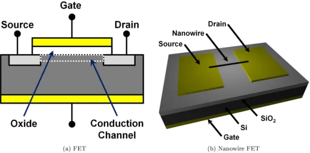
impedance, that can be processed directly. This well-represented class of sensors is summarized elsewhere [34, 35]. The most promising among these devices is the nanowire eld eect transistors (FET). FETs are devices that monitor the current between two electrical terminals, called the source and drain, embedded in a semiconductor. A second electric eld can be applied across two terminals oriented orthogonal to the source to change the concentration of charge carriers (electrons or electron holes) in the semiconductor and gate the current that reaches the drain. Figure 2.5a illustrates this principle.

A FET biosensor is composed of a semiconductor connecting the source and drain electrodes. Charged biomolecules that adsorb to the semiconductor sensor produce an electric eld that acts as the gate and changes the charge carrier density within the device. The resulting drain current can be conveniently measured as a reporter for sensing applications. This type of device has been widely applied [34]. Its LOD is generally greater than 1 nM for most biomolecules because the electric eld from the bound species only penetrates to a limited depth within the conduction channel. This problem is partly overcome by the use of nanoscale objects to bridge the source and drain such as carbon nanotubes [36, 37] or lithographically dened nanowires [38, 39]. The increased surface area-to-volume ratio for these structures allows the electric eld due to adsorbed material to perturb a larger portion of the conduction channel, yielding an LOD low enough to allow for the detection of single virus particles [40]. Figure 2.5b depicts a generic nanowire FET biosensor.

In addition to being a sensitive label-free technology,nanowire FET biosensors can be produced relatively cheaply in parallel with traditional microfabrication techniques that are common in the semiconductor in- dustry. These devices are well suited for incorporation into microuidic ow cells, and they are suciently small to require only microliters of sample for a measurement. While the small sensor size aords a number of advantages, it also poses challenges when integrated in microuidic systems. Sensing requires molecular interaction with the surface where, in the laminar ow of a microuidic channel, the velocity is zero.

Moreover, the high pressure drop in small channels limits the velocity of the ow and, thereby, the transient response of the sensing system.

The performance of most nanowire FET biosensors decays in the presence of salts. Most biomolecules

(42)

(a) FET (b) Nanowire FET

Figure 2.5: Field eect transistors (FETs). (a) A generic FET, including the source and drain with conduction channel between the two. A eld applied using the gate can control the density of charge carriers in the conduction channel and change the current measured at the drain. (b) A nanowire eld eect transistor (FET) sensor. Biomolecules bound to the surface of the nanowire have a localized electric eld that can distort the charge carrier density in the nanowire. Changes in the drain current are used to track how much material has adsorbed to the device.

require a buered environment to screen interactions that would cause the molecules to precipitate and to stabilize their structure, so a pH-buered salt solution is often used to dissolve samples of known analyte.

Even biouids like blood or saliva have their own salts and buering agents for this purpose. These salts screen the electric eld of the biomolcule, reducing its eect on the charge carrier population in the conductor [41], thereby limiting the sensitivity in biologically relevant uids. This negates the eld eect provided by the adsorbed material and limits the sensitivity in biologically relevant uids.

The surface-bound molecular recognition species that enable specic sensing can also diminish the performance of nanowire FET biosensors due to screening eects. Such surface modications can either promote or retard conduction, depending on the electrical properties of the nanowire. Some functionalization schemes can even modify the charge state of the nanowire permanently [27] and alter the fundamental electrical properties of the device. Identifying methods suitable for nanowire FET sensors remains a challenge.

Recently, however, a clever technique has been used to improve the applicability of these devices [42]. In this method, a two-stage ow system allows the sample to enter a chamber where an immobilized molecular

(43)

recognition species can remove the analyte of interest through specic binding. The liquid in the chamber is then ushed and replaced with a low-salt buer, creating an environment that promotes gradual dissociation of the analyte. This resulting solution is then driven into a second chamber where the nanowire FET sensor is located. The analyte is then free to interact with the sensor in the absence of unwanted species that may have been present in the original sample liquid while also removing the need for functionalizing the surface of the biosensor.

Mechanical Biosensors

Some biosensors use mechanical forces and motion to report the amount of analyte present in a sample.

One important example of such a device is the microcantilever [43], which may be used in two modes of detection. First, the static deection of these devices that results from specic adsorption can be used to measure analyte concentration [44]. Alternatively, the microcantilevers oscillate at a characteristic frequency, much like a tuning fork. This frequency is a function of the shape and material properties of the cantilever, and therefore changes upon adsorption of biomolecules. The deection and the cha