In the third chapter we review the evolution of the perturbations in the adiabatic model. The fifth chapter examines the observational signatures of the isocurvature perturbations in the CMB anisotropies.
Brief overview
- The expansion of the universe (Hubble’s law)
- Light element abundances
- Cosmic microwave background radiation
- Evolution and distribution of galaxies
Since its accidental discovery by Arno Penzias and Robert Wilson in the CMB, radiation has been considered a hallmark of the Big Bang model. The smoothness of the CMB confirmed that the universe had previously undergone a brief period of rapid exponential expansion, called inflation.
Age and energy contents of the universe
Cold dark matter plays a key role in the structure formation and evolution of galaxies, and has influences on CMB anisotropies [69].
Background and perturbed Friedmann-Robertson-Walker models
The “vector mode” corresponds to the transverse vector parts of the metric, found in Bi⊥ and Eij⊥. The conformal Newtonian gauge is a simple measure for scalar modes of the metric perturbations, but can be generalized to include vector and tensor modes [19].
Einstein equations and energy momentum conservation
Equation (2.15) shows that the acceleration of the expansion of the universe is due to the density and pressure filling the universe, where positive acceleration requires a component of negative pressure P <¯ −ρ/3.¯. The matter components of the universe (baryons and cold dark matter) can at all times be treated as ideal fluid, which allows to be completely described by the energy density contrast δ and the velocity divergence θ, while for the radiation components (neutrinos and photons), a full treatment requires the use of the Boltzmann equation.
Initial conditions
- Large scales
- Super-horizon solution
- Through horizon crossing
- Small scales
- Horizon crossing
- Sub-horizon evolution
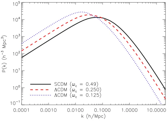
- Matter transfer function and Power spectrum
- Growth function
- Including other species
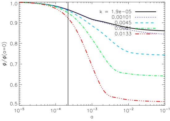
Equation (3.31) describes the evolution of the gravitational potential for modes crossing the horizon in the radiation-dominated epoch. With the knowledge of the gravitational potential in the radiation-dominated epoch, let us solve the problem of perturbation evolution.
Evolution of photons and baryons prior to decoupling
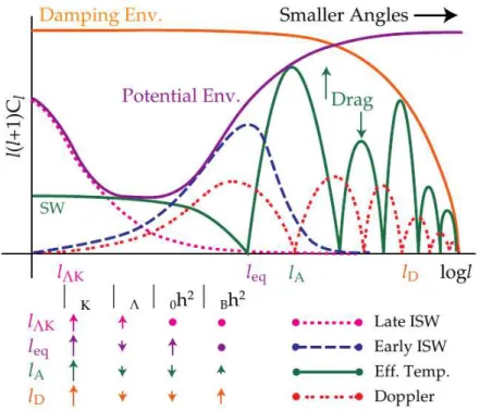
The ordinary Sachs-Wolfe effect
Therefore, the only nonzero terms in equation (4.8) are the internal photon density contrast at the final scattering surface and the Newtonian gravitational potential. This effect is the dominant source of fluctuations in the CMB for angular scales above about ten degrees (large angular scales i.e.
The Doppler effect
The integrated Sachs-Wolfe effect
Boltzmann Hierarchy and the line of sight integral approach
Line of sight integral approach
In terms of the source function, the multipole moments Θℓ(k, τ) are given by Θℓ(k, τ) Equation (4.41) also shows that the anisotropy that we measure today can be seen as a spherical projection through the spherical Bessel function of fluctuations on the last scattering surface towards us The expression of the source function in the synchronous gauge, which corresponds to the expression in the conformal Newtonian gauge given in equation (4.40), can be easily derived knowing that the conformal Newtonian potentials φ and ψ are related to the synchronous potentials that are in k-space using the set of equations (2.9), and the photon density contrasts,δγ and the baryon velocity divergencesθb in both conformal and synchronous gauge are related by equations (2.10) and (2.11).Show in the following section, the photon polarization contribution to the source function is small and can be neglected for the primary anisotropy.
This tells us about the strength of temperature anisotropies on a given angular scale∝1/ℓand can be written as.
CMB anisotropies
Transfer function ∆ ℓ (k)
So in this approach (equation (4.54)), the evaluation of the multipole moments only requires the knowledge of the fluctuations at photon-baryon decoupling, and the time evolution of the potential from the last scattering surface to our present day. The Bessel functionjℓ(k) tells us how much anisotropy on large scales is contributed by a plane wave with wavenumber. As the limit of the Bessel function vanishes for very largeℓ (very small angular scales), the transfer function vanishes.
Angular power spectrum C ℓ
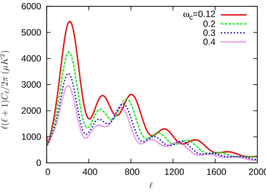
Effect of cosmological parameters on the CMB temperature spectrum: adiabatic case 57
- Matter density Ω m h 2
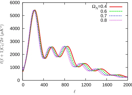
- Cosmological constant density Ω Λ
- Curvature density Ω K
- Optical depth τ e
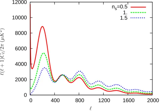
- Spectral index n s
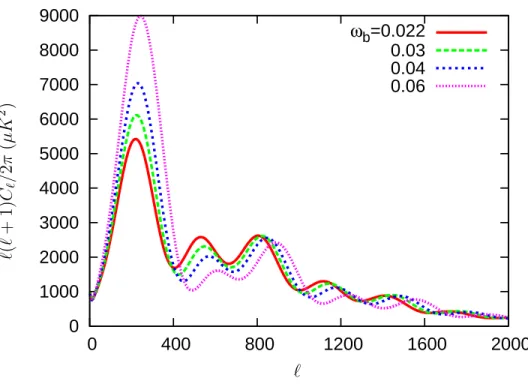
The baryon density is the cosmological parameter that has the most influence on the heights and locations of peaks in the CMB power spectrum. Therefore, the effect of the cosmological constant on the CMB power spectrum is only due to the milling of photons from the last scattering surface towards us. Figure (4.4) shows how the CMB power spectrum is shifted to larger scales as we increase the cosmological constant.
For other wavenumbers, ns will change the slope of the CMB power spectrum by rotating around some multipoleℓp ≃ kpτ0.
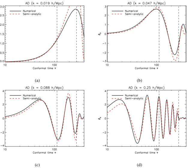
Evolution of photon and baryon perturbations
Evolution of photons and baryons prior to decoupling
- AD mode
- NID mode
- NIV mode
- CI & BI modes
We consider the time evolution of the photon-baryon fluid in the tight coupling regime. Thus, the time evolution of the acoustic waves in the photon component before decoupling is given by. The time evolution of the photon and baryon density contrasts for the NID mode is given by.
The time evolution of the photon and baryon density contrasts for the CI and BI modes is given.

CMB anisotropies in isocurvature models
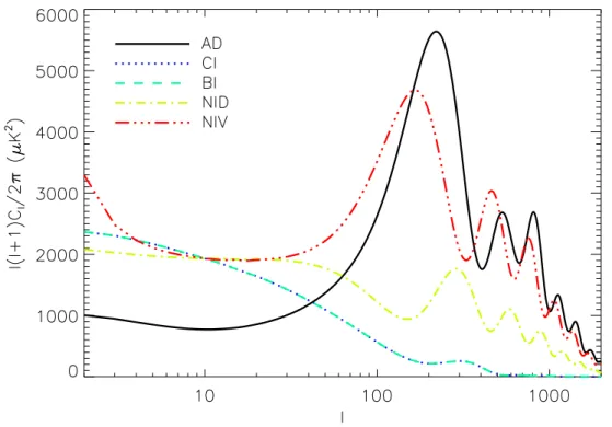
We can see that the approximation reproduces the main features of the CMB power spectrum. The contribution of the ISW effect around the first peak in the NIV mode is not as important as in the AD mode due to the smallness of the gravitational potential and its time derivative. In Fig. 5.17 we present the different contributions to the CMB power spectrum for the NIV mode.
As ℓ increases, the contribution due to the change in gravitational potential decreases and the usual SW contribution becomes dominant in the transfer function.
Effect of cosmological parameters on the isocurvature CMB temperature power spectrum100
- Matter density Ω m h 2
- Cosmological constant density Ω Λ
- Curvature density Ω K
- Optical depth τ e
- Spectral index n s
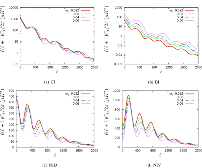
In this section, we study the effect of each of the above cosmological parameters on the CMB power spectrum in isocurvature modes. The effect of the other cosmological parameters on the CMB spectrum in isocurvature models is similar to the AD case. Changing ΩΛ affects the CMB spectrum, but its effect is negligible compared to the effect of the matter density itself.
The effect of changing the cosmological constant density on the temperature power spectrum of the CMB in the isocurvature modes is similar to the AD case.
The BAO peak with adiabatic and isocurvature initial conditions
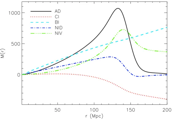
To quantify the shifts in the BAO peak of the isocurvature modes relative to the adiabatic mode, we plot in Figure 6.1 the baryon mass profile [47] of the different modes at decoupling, defined by. We observe that the BAO features for the isocurvature modes differ in shape and position from the adiabatic BAO peak, due to the effect of the diffusion damping on the undamped BAO profiles discussed earlier. In the case of the NID and NIV modes, there is a pronounced peak offset from the adiabatic BAO peak due to the coupling to different harmonics, as described above.
It is also interesting to note that the amplitude of the mass perturbation at the origin is much smaller for the isocurvature modes, because the curvature, and thus the mass fluctuation, is initially unperturbed.
Dark energy constraints
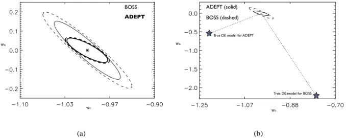
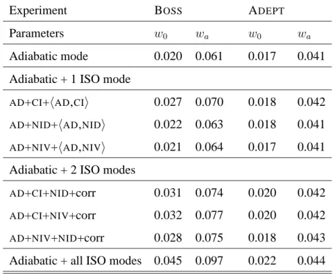
This dark energy model is shown by the dotted lines for each of the two experiments considered. Note that for the calculation of the PLANCK Fisher matrix, we follow Al-brecht et al and reintroduce the strict geometric degeneracy between the dark energy density ΩX and w0, which can be artificially broken in the standard Fisher matrix calculation, leading to error underestimations . The question we wish to ask is, what bias in the estimates of dark energy parameters can be caused by wrongly assuming adiabaticity.
Furthermore, even in the case of a single isocurvature mode correlated with the adiabatic mode, deviations from scale invariance and a scale-dependent correlation can cause further deterioration of the constraints presented here.
Conclusions
Introduction
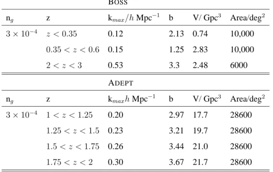
In this chapter, we explain in depth why small amplitude but general mixing of correlated isocurvature modes can have such a strong impact on the cosmological constraints based on BAO surveys. The isocurvature modes excite different harmonics, which in turn couple differently to Silk damping, thereby modifying both the scale on which the sound waves characterize the baryon distribution and the shape of the BAO peak. In Section 7.3, a Fisher matrix formalism is implemented to quantify the impact of these changes on the predicted errors on the dark energy parameters from two BAO experiments, namely BOSS [48] and ADEPT [151].
Finally, we show that constraints on the isocurvature parameters can be derived from BAO studies.
The BAO peak with adiabatic and isocurvature initial conditions
- AD mode
- NID mode
- NIV mode
- CI & BI modes
- Time evolution of the BAO peak position
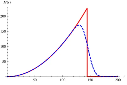
Due to the shape of the invincible mass profile (no baryons on scales larger than the sonic horizon), the damping of silk. The redshift evolution of the mass profile for the AD mode has been previously studied in the literature [ 47 ]. The time evolution of the photon and baryon density contrasts for the NID mode are given by.
The time evolution of the photon and baryon density contrasts for the NIV mode is given by.
Impact of isocurvature modes on dark energy constraints
Statistical Formalism
- Large Scale Structure (LSS) surveys
- Cosmic microwave background (CMB) surveys
The BAO peak manifests itself as oscillations in the matter power spectrum, with the size of the sound horizon determining the frequency of these oscillations. The first source of information is the acoustic oscillations of baryons, where their wavenumber k = 2π/rs is determined by the size of the sound horizon at decoupling rs. Assuming that the probability function of the band powers of the galaxy power spectrum is Gaussian, the Fisher matrix can be approximated as follows:
Derivatives of the power spectrum with respect to the cosmological parameters in Table 7.1 and to the isocurvature parameters are shown in Figures A.1 and A.2 in the Appendix.
The impact of isocurvature modes on dark energy
- Constraints on isocurvature modes from the LSS data
We first consider the case of a mixture of adiabatic mode and isocurvature mode CDM. In Fig. 7.14 we compare the sum of the most dominant isocurvature contributions zhAD,NIViPhAD,NIVi + zhAD,NIDiPhAD,NIDi to the power spectrum at different redshift bins of the BOSS experiment with their error bars. Clearly, this combination of isocurvature parameters is best constrained by the measurement of the galaxy power spectrum at z = 0.6 for this particular experiment.
Hence, measuring the BAO scale at different redshifts between decoupling and today helps to constrain the isocurvature modes.
Conclusions
We also assessed the effect of the cosmological parameters on the CMB temperature power spectrum in AD mode. We focused on the impact of baryon density and matter density on the CMB power spectrum. In the fifth chapter, we investigated the characteristics of the isocurvature CMB power spectra and studied the impact of various cosmological parameters on the CMB power spectrum.
However, the BAO data in turn provide significantly stronger constraints on the nature of the primordial disturbances.