This is required by New Zealand law, under the Hazardous Substances and New Organisms Act (HSNO) 1996. The Te Mana Ruhī Taiao Environmental Protection Authority (EPA) processes and assesses all applications for new hazardous substances.
Introduction
- Context
- Purpose
- The role of the risk assessment
- Using this document: a flexible approach
- Future updates
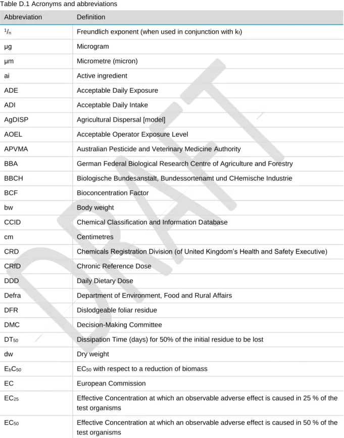
- Glossary
It is assumed that users of this document already have a fairly good understanding of the approval application process for new hazardous substances in New Zealand. Finally, this document contains our current approach to assessing and evaluating the risks, costs and benefits of new hazardous substances in New Zealand, and is intended to be a living document.
How hazardous is the substance?
- The New Zealand hazard classification system
- How to classify the substance
- Classification using data from scientific studies
- Classification by mixture rules
- Exceptions
- Can an existing approval apply?
- For help classifying your substance
More information on the type of studies required can be found in the data requirements section of the EPA website (EPA, 2016b, 2018b). The controls (or restrictions) assigned for the use of the new hazardous substance in New Zealand must be the same as the group standard or existing approved substance to which the new substance is adapted.
Assessing the risk
Understanding exposure paths during the life cycle of the substance
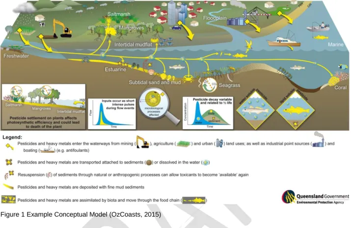
Ultimately, a robust risk assessment is based on the development of conceptual models to predict the effect of the release of the hazardous substance. It also affects the routes of exposure, whereby receptors can become vulnerable to the dangerous substance.
Qualitative assessment
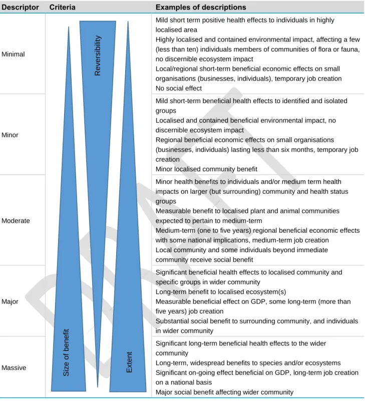
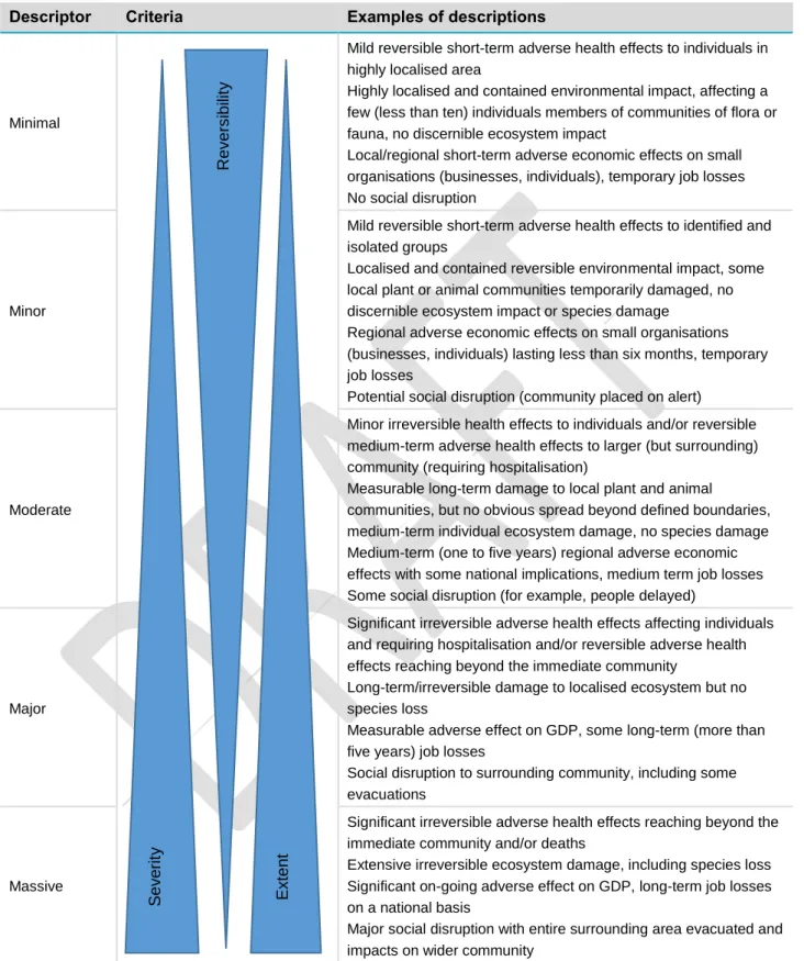
- Qualitative descriptors: standard language to use in a qualitative risk assessment15
- Quantitative models used by the EPA
- Selecting inputs for quantitative models
- Understanding uncertainty in quantitative models
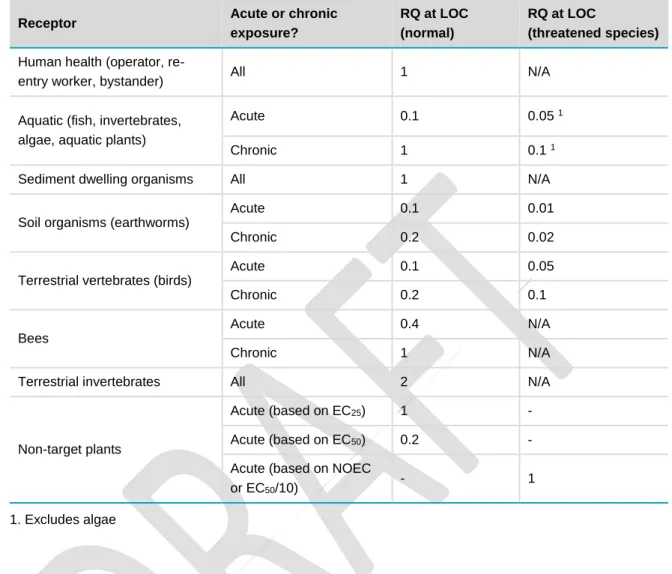
- Threatened and ‘at risk’ species
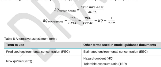
- Standardising terminology and using quantitative model outputs
- Data made available to other regulatory agencies
The chance or probability that the event will occur (expressed as a number between 0 and 1 or 0 and 100%). For those models that do not use 'risk quotients', the original term should be used when refining the model output within the framework of the relevant guidance document, and the final output should then be converted to a 'risk quotient'.
Controls
The purpose of controls
Prescribed controls
Modified/additional controls
Benefits assessment
The importance of understanding the benefits
Who is responsible for collating this information?
What to include in a benefits assessment
Choice What is the advantage for families of being able to live and work in an area of their choice? What are the additional costs of alternative recreation, because this is the advantage of keeping the current one. The more detailed quantitative assessment is generally only required if the qualitative assessment of the benefits, or the balance of benefits and risks, indicates that the applicant needs further work to confirm that the benefits outweigh the risks.
Reaching a decision on a hazardous substance
The time frame of when the risks, costs and benefits are likely to occur is also an important consideration. Assessing the combined assessments of risks, costs and benefits for the purposes of deciding whether an application should be approved, conditionally approved or refused. An estimate of the intrinsic properties of a substance that do not change with volume or exposure.
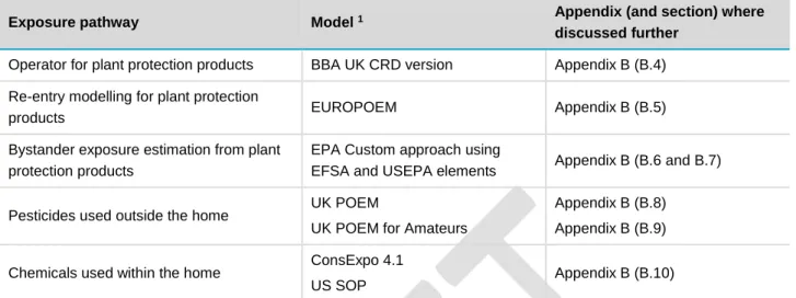
Introduction to human health modelling
Acceptable Operator Exposure Level
Dermal absorption
Commercial pesticide operators
The UK CRD exposure model calculates exposure using the results of actual measurements carried out in the field (Chemicals Regulation Directorate, 2016a). The UK CRD version of the BBA operator exposure model calculates exposure from the results of actual measurements carried out in the field (Chemicals Regulation Directorate, 2016a). These protection factors are based on the 2014 EFSA exposure model (EFSA, 2014) and are detailed in Table B.4 below.
Re-entry workers
It is important to verify that returnee activity matches this assumption before using this model. These are seen as independent of the active substance/product used and depend on the crop type and the activity performed by the re-entry worker (EUROPOEM, 2002). These transfer coefficients all assume that returners wear long pants and a long-sleeved shirt and do not wear gloves.
Bystanders to commercial pesticide use
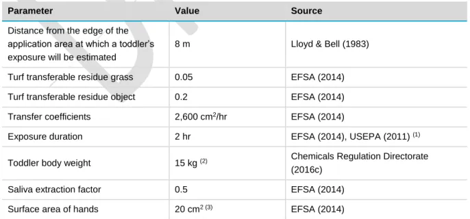
A small child is assumed to be exposed to all the spray that is deposited on a surface. There is also the potential for spectators to be 'residents' and have a longer exposure. Distance from the edge of the application area where a young child's exposure will be estimated.
Bystanders to recreation land and residential pesticide use
Please see section B.4.8 for reasons why the 2014 EFSA operator, worker, resident and bystander exposure model is not used. There are a number of other models for assessing risks to people at home. UK POEM and UK POEM for amateurs (see sections B.8 and B.9 respectively) consider the risks to home operators and are therefore not relevant to this pathway.
Outdoor home-use concentrated pesticides
To assess the risk from recreational exposure, i.e. exposure of young children to a surface such as a lawn or sports field treated with pesticides, the approach in Equation B.15 is used with updated default parameters from Table B.9 used in Equation B. .10 k equations B.13. The risk quotient approach is used in risk assessment for private users of pesticide concentrates outside the home (see equation B.1). The UK POEM for amateurs (see section B.9) considers the risks to home users from diluted ready-to-use products and would therefore underestimate the risks of this route.
Outdoor home-use diluted pesticides
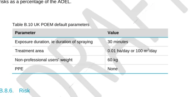
Although the spreadsheets will also calculate the risks as a percentage of the AOEL if an AOEL value is entered, the EPA prefers not to use this option. The risk quotient approach is used to determine the risks for the private users of concentrated pesticides outside the home (see Equation B.1). UK POEM (see section B.8) considers the risks to home use operators of concentrated products and is therefore likely to overestimate the risks of this pathway.
Indoor chemicals
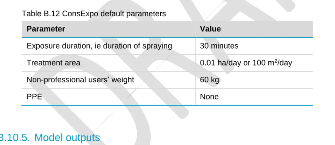
With a longer interest in energy efficiency in Europe, these are likely to be conservative for New Zealand homes. The default setting of the model assumes that the chemicals are non-volatile and this needs to be confirmed for each substance. Caution should be exercised with the US units in the model due to New Zealand's metric system.
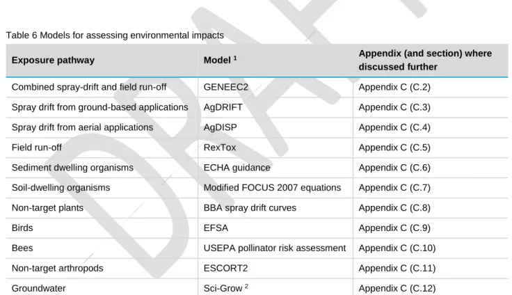
Introduction to environmental modelling
Aquatic risk assessment (combined spray drift and run-off)
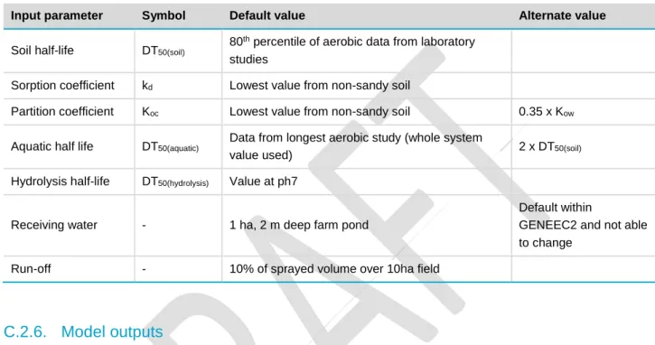
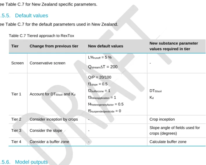
In the absence of any study data, default parameters from the GENEEC2 guidance document (USEPA, 2001) are used, as shown in Table C.1. The GENEEC2 model outputs a text file summarizing input parameters, half-life values of the active ingredient in various environmental media, estimated environmental peak concentrations (EECs), and EECs calculated at a number of different time steps (four , 21, 60 and 90 days). This result should be summarized in the accompanying report, using the term predicted environmental concentration (PEC) as explained in Table 10 and section 3.3.5.
Aquatic environment (refined ground-based spray drift)
Based on the extent of the empirical studies behind the spray drift data, the buffer zone limit in the model is 254 m. The parameter values in Table C.2 are used as defaults in the refined aquatic assessment for spray drift from ground-based equipment. This information is then used, along with the data from the APVMA spray drift curves and related lookup tables, to calculate the buffer zone required to reduce the ambient concentration to an acceptable level.

Aquatic environment (refined aerial-based spray drift)
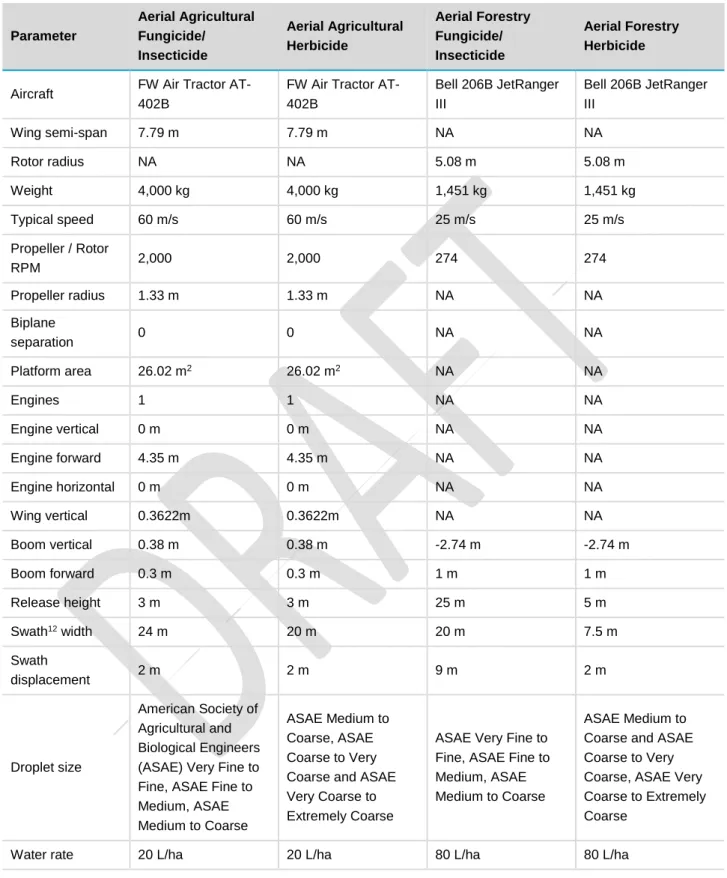
If the applicant is able to produce an alternative spray drift data set that is collected using international best practice and is considered acceptable, these data can be used for the exposure assessment. The air component used in AgDISP has been well validated, although it has been shown to overpredict spray operation at distances greater than 100 m and underpredict spray operation at distances less than 100 m. The parameter values in Table C.6 are used as default in the refined aquatic assessment for spray operation from fixed boom equipment.
Aquatic environment (refined runoff)
The final level involves rearranging Equation C.8 into Equation C.12 to find the buffer zone ('buffer width') required for the RQ to be less than the level of concern in Table 9. The output of Level 4 is a buffer zone size required for to reduce the risk quotients to an acceptable level. If the risk cannot be discounted beyond the third level, the buffer zone needed to reduce the predicted concentration down to an acceptable level is also a measure of the level of risk; with the larger the buffer zone, the higher the risk.
Sediment organisms
When results from whole sediment tests with benthic organisms are available, the Predicted No Effect Concentration in Sediment (PNECsediment) should be derived from these tests using assessment factors. The assessment factors in Table C.8 are used to account for the uncertainties of the number and variety of available sediment-dwelling test data. The only New Zealand specific parameters used in this assessment relate to the use of the substance under assessment.
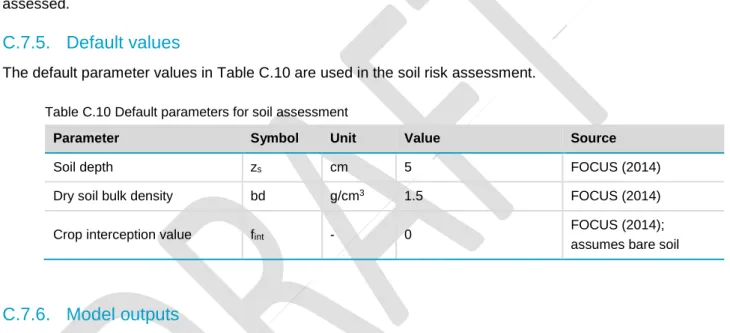
Soil organisms
Initial PEC concentrations from the FOCUS guideline are used instead of their time-weighted average approach for acute and chronic risks. For off-field calculations, the 90th percentile of spray displacement values from the BBA model for ground booms and AgDISP for aerial applications are used. The results of the calculations are the estimated exposure concentrations provided by the corresponding PEC values from equation C.15 to equation C.18.
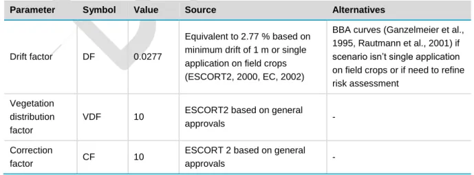
Non-target plants
Spray curve data from the BBA (Ganzelmeier et al., 1995, Rautmann et al., 2001) are used in this model, although the spray drift curves from the Spray Drift Task Force are also used in the AgDRIFT model. The predicted concentrations from the BBA operating curves in Section C.8.5 are used as an estimate for planters. Spray curve data from the BBA (Ganzelmeier et al. 1995, Rautmann et al. 2001) are used in this model, although the spray drift curves from the Spray Drift Task Force are also used in the AgDRIFT model.
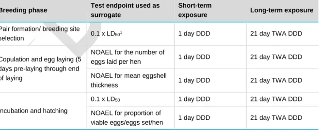
Terrestrial vertebrates
The risk of secondary poisoning may also be considered if there are concerns based on the molecular size of the component. It is assumed that the relevant indicator species feeds only on contaminated food and the concentration of pesticide on the food is not affected by the growth stage of the crop. In contrast, the EFSA bird model is a deterministic model which uses a single iteration of the relevant equations with a single value for each parameter.
Pollinators
These limitations also apply when incorporating USEPA's modified Briggs approach is used in New Zealand. The different dietary requirements of different larvae and adult castes are taken into account while calculating dietary doses. The risk quotient (RQ) approach is used to estimate risks for individuals within each brood caste.

Non-target invertebrates
The default values presented in Table C.14 are used in the assessment of non-target beneficial insects. When performing limit tests, a low risk to non-target arthropods can be inferred when the effects at the highest application rate, according to Equation C.25, are below 50 % (ESCORT2 workshop, 2000 – p12). The ESCORT2 model is the only approach considered by the EPA to date for the exposure of, and risks to, non-target invertebrates.
Groundwater
HSE, [undated-b], http://www.hse.gov.uk/pesticides/topics/pesticide-approvals/pesticides-registration/data-requirements-handbook/operator-exposure.htm. Environmental Protection Agency, Washington DC, https://www.epa.gov/sites/production/files/2015-08/documents/usepa-opp-hed_residential_sops_oct2012.pdf, accessed 03/16/2017. Department of Pesticide Regulation; https://www.epa.gov/pollinator-protection/pollinator-risk-assessment-guidance, accessed 03/16/2017.