This must be distinguished from a tax progressivity, which refers to the redistributive properties of the tax. In this case, the tax rate is expressed as a ratio of the price before tax.
Principles of Good Tax Policy
These characteristics of a good tax system are similarly reflected in the Henry Review for Australia. In any case, they should not be the legal or economic designers of the tax system.
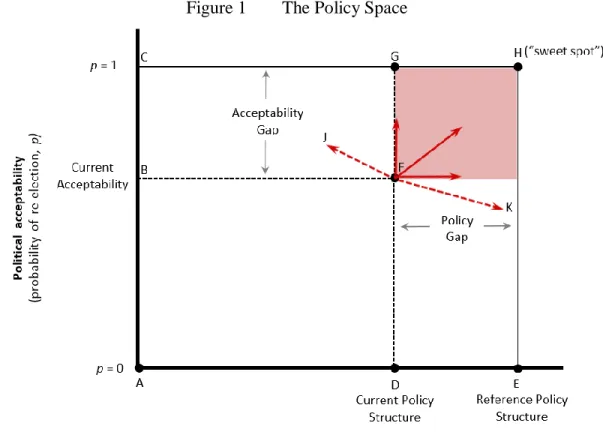
Rational Policy Analysis versus Political Priorities
Of course, almost no policy is likely to be perceived as a guarantee of re-election (on the CH line). In this sense, policy options moving directly to the northeast are likely to be most successful.
Some Simple Lessons from Economics
- Legal and Economic Incidences Often Differ
- People, Not Companies, Pay Tax
- Consider Taxes Within a Broader Set of Policy Options
- Taxes have Intended and Unintended Consequences
- The Coherence or ‘Congruence’ of the Tax System matters
- Taxes and Expenditures Need to be Considered Together
- No Observed Change Does Not Mean No Effect
- A Taxpayer Can Respond to a Tax Change of which They are Unaware
- Microeconomic and Macroeconomic Approaches to Tax Policy can Conflict
The regressive effect may not have been intended, but it had a by-product effect of clashing with redistributive goals of the tax system. Claus and Sloan (2008) provide an evaluation, and Brook (2011) some discussion, of the macroeconomic case in the New Zealand context.
Fifteen Lessons from Tax Analysis
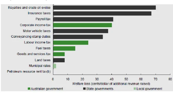
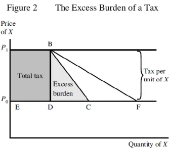
Welfare Losses are the Most Comprehensive Metric of the Costs of Taxation
However, the fall in demand along the (‘Marshallian’) demand curve segment, FB, includes the loss of income due to the tax paid, while the excess burden measure should take into account the income compensation discussed above. As a result, the excess tax burden is measured by the area of the smaller triangle, BCD, rather than by the BFD. But they serve to emphasize the orders of magnitude these welfare measures of the tax system can produce, as well as the differences between taxes.
In particular, where effective marginal tax rates are high – which can apply at both the bottom and the top of the tax scheme due to interactions with social transfer systems – excess income tax burdens can be particularly important for tax policymaking.
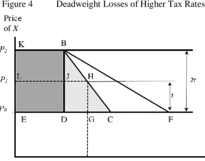
Deadweight Costs of Taxes Increase Disproportionately with Higher Tax Rates
2012) and Hendren and Sprung-Keyser (2019) provide two calculations of excess burdens for the highest income tax rates in the United States. The above results highlight that the efficiency costs of setting high income tax rates need to be carefully assessed to be situation and tax system specific, but can be very high in some circumstances. So if the unit tax doubles from t to 2t, the excess burden is four times greater.35 Note also that revenue will less than double at KBDE (which is less than twice LHGE) when the tax rate doubles.
If behavior adjusts less in response to a tax increase (after allowing for appropriate income compensation), we can often be less concerned about possible efficiency costs (but see 2.7 above).
Policy to Minimise Distortion Costs Should Equate MWCs Across Different Taxes The intuition behind this result is fairly straightforward; namely that if the welfare costs per
The inverse elasticity rule, associated with Ramsey (1927), shows that, under certain conditions (which include ignoring distributional objectives), indirect tax rates should be set in inverse proportion to their elasticity of demand. It is important to recognize, as discussed further in 3.13 below, that this result, where optimal rates of indirect taxes could be set by reference to their efficiency and distributional characteristics, lies in the absence of income tax. Other results in the literature, notably Atkinson and Stiglitz (1976), following Diamond and Mirrlees (1971a,b) and Diamond (1975), show that setting different tax rates for goods according to their distributional characteristics may be inferior to uniform rates when a progressive income tax is feasible.
However, with a relatively high aversion to inequality, tax rates on those commodities would be lowered instead.
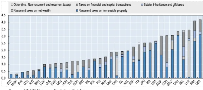
Avoid Taxing Transactions
Following the reforms of the 1990s, New Zealand has almost no such taxes, while countries such as Australia, the United Kingdom ('GBR'), Italy and Turkey rely relatively heavily on them. Best and Kleven (2018) examined the responses of the UK housing market to the UK Property Transaction Tax (Stamp) and the presence of "notches" in its structure. Secondly, partly due to the first effect: "temporary reduction of the transaction tax is an extremely effective form of fiscal stimulus.
A temporary repeal of a 1% transaction tax has boosted housing market activity by 20% in the near term (thanks to timing and extensive responses)”;
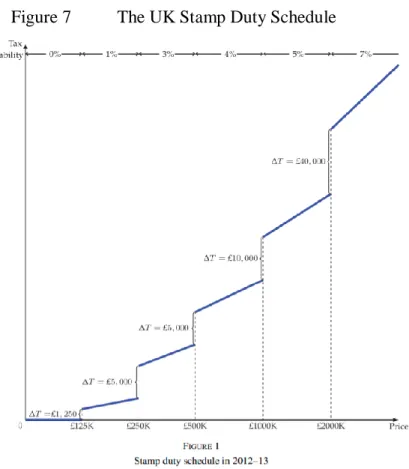
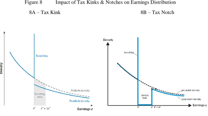
Minimise ‘Kinks’ and Avoid ‘Notches’ in Tax Schedules
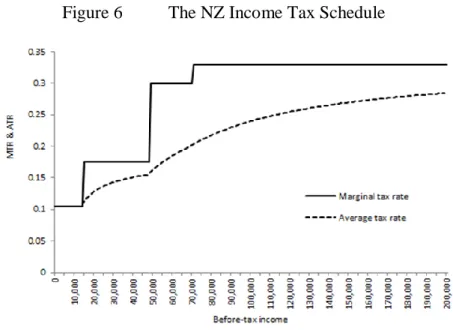
Such income shifting is more likely (and more rewarding for the taxpayer) where there are large, discrete changes in marginal tax rates, MTRs ('kinks'), and particularly where there are large discrete changes in average tax rates, ATRs ('notches'). in the tax list. Until December 2014, these percentage rates were charged on the total sales price, rather than on the price above each threshold in the list.37. Of course, in practice such grouping is never so precise and taxpayer 'peaks' in the income distribution are usually observed around tax thresholds.38.
The main difference is that no one is expected to settle in the segment just above the threshold (labelled the 'density hole') - the income levels where they would be worse off after tax - and instead crowd in just below.
Avoid Taxing Income Differently when Earned Through Different Legal Forms Just as taxing different goods and services at different rates of GST creates tax-induced
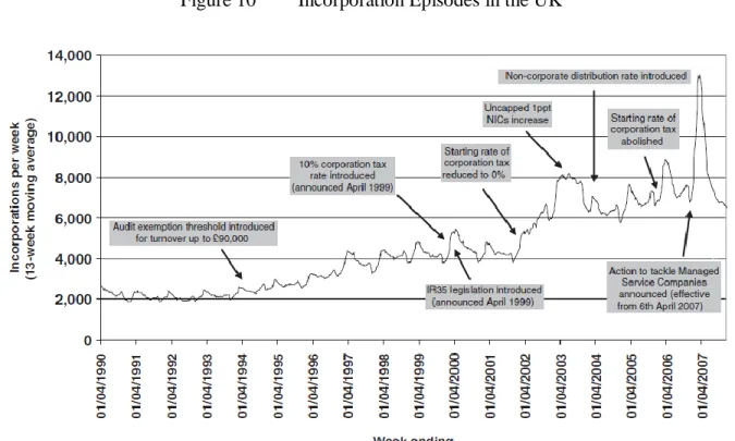
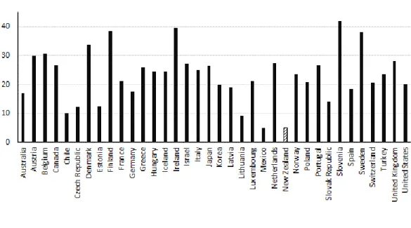
Nevertheless, as Figure 9 shows, after the top personal rate was again reduced to 33% in 2011, the difference between the personal and business rates in 2018 was only 5 percentage points. Other OECD countries, by contrast, typically have a 15-25 percentage point difference in these rates, with some, such as Ireland, having a business rate almost 40 percentage points below the highest personal rate. NZTWG (2018b, section 4) and Gemmell (2020) show that after the top personal tax rate and the trust rate were 'adjusted' to 33% in 2010, but the corporate rate was not adjusted, there were noticeably divergent trends between income earned through trusts and income , which goes through small closely-held companies.
They note that 'after the increase in the top personal rate in 2000, the number of corporate income tax returns has increased by almost 10% p.a.
Achieving Tax Efficiency Should Include Administrative and Compliance Costs The tax reviews discussed in section 2 highlighted tax policy objectives that include maximising
In this context, the main variable that is increasingly used empirically to measure the impact of tax rate (income) changes on behavior (and taxpayer welfare in some circumstances) is the elasticity of taxable income (and hence of revenue) to changes in the tax rate.41 This can be extended to include an 'elasticity of tax revenue enforcement': the response of revenue to an administrative intervention, such as increased auditing, third-party reporting, pre-population of returns tax, etc. An essential feature of these models, therefore, is that neither the elasticity of taxable income nor the elasticity of enforcement are invariant.42 Thus, if taxpayer responses to a change in tax rates appear undesirable – for example due to evasion – it can be the change of the law and administrative. the tax structure can change one or both of these elasticities in desired directions. 41 Following Feldstein (1995) elasticity is usually defined in terms of '1 minus the (marginal) tax rate' so that it is expected to be positive.
42 This contrasts with the elasticity of labor supply with respect to, for example, tax rates, which is typically modeled as the result of (invariant) preferences between work and leisure.
It is Sensible to Use Either Households or Individuals as the Tax Base, but not Both Setting tax policy inevitably involves inter-personal comparisons, raising the question: how
Furthermore, the resources used for this enforcement of compliance will usually be drawn from another productive activity, so that the total resources in the economy may be lower – if the compliance activity is less productive than the alternative it has replaced. For these reasons, there is no single number or ROI that can identify the "correct" allocation of funds to meet tax regulations. Where the resources used to enforce compliance would otherwise be useless, the costs may be low, but they can be very high if productive private sector activity is displaced.
It makes little sense to provide the same financial safety net to low-income or unemployed people who live in a wealthy family as well as to people who do not have such a family.
Don’t Hypothecate Individual Taxes to Specific Public Spending Items
Since the supply of land is perfectly inelastic (fixed in supply), market prices depend on what buyers are willing to pay and not on the expenditure of landowners. This can then be associated with a relatively low elasticity of land supply in production (use). If land is truly fixed in (economic) supply, then any change in land taxation should be reflected in a proportional change in its price.
That is, the tax must be 'fully capitalized' into the land price - a 10% tax on the value of land that generates a 10% fall in the land price.
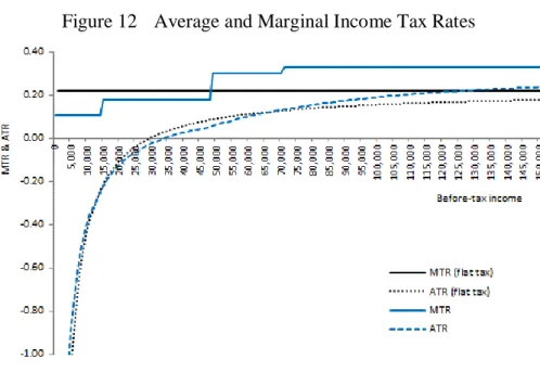
Rather, the extent of redistribution depends on (a) how far the average tax rate (ATR) rises with income; and (b) how many people are affected by each rate – the shape of the pre-tax income distribution. This slightly larger transfer amount in the flat tax case allows a closer alignment of the ATRs in the two cases, but is not decisive. Thus, the extent of progressivity of the income tax and transfer system in both cases is very similar despite a single MTR in one case.
This message is reinforced when looking at the average income tax burden across deciles of income distribution; see NZTWG (2018a, p.7).
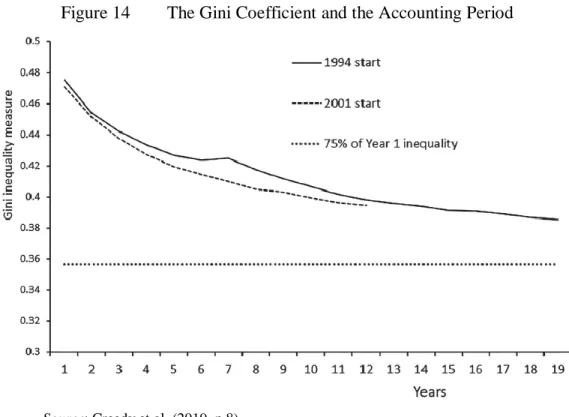
Some Taxes Redistribute Income More Over the Life Cycle than across Individuals All OECD governments use tax policy variously to redistribute income from higher to lower
This indicates that, on average within each of the lowest four deciles of personal income distribution, income taxes paid (less cash transfers received from government) as a percentage of income are negative (taxpayers are net recipients, not payers, of income tax /income transfers), with the fifth decile paying almost zero net income tax. The OECD "tax wedge" is defined as the sum of personal income tax and social contributions paid by employees and employers, less benefits, as a percentage of employers' labor costs. For example, this shows that Gini's lifetime gross income is only about 57% of its equivalent annual value.
In Figure 15B, the intrapersonal redistribution share per decile, excluding the lowest two and the highest, across deciles appears similar to the average for all individuals: approximately 55-60%.
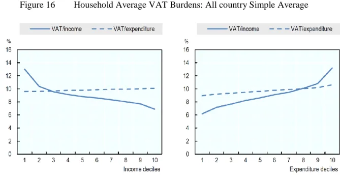
Don’t use VAT (GST) as a Redistributive Tax
These results should give fiscal policymakers pause for thought, as they suggest that, contrary to a common assumption, more than half of the apparent annual redistribution achieved by the tax and benefit system may simply be reallocate income over time to the same individuals rather than from the long-term or lifelong rich to the lifelong poor. VAT regimes in most of the 27 OECD countries also typically have significant exemptions to lower tax rates for redistributive reasons. The results by decile of expenditure for the case of universal cash transfers ('reform 2') are shown in Figure 17.57 Despite the fact that the cash transfer is paid to all consumers/taxpayers, the transfers manage to generate significant net gains for the lowest 5 deciles at the expense of the highest deciles.
Thus, non-uniform VAT rates appear to be a highly inefficient way of increasing the incomes and expenses of the poorest consumers, compared to a simple system of remittances (or "universal basic income").
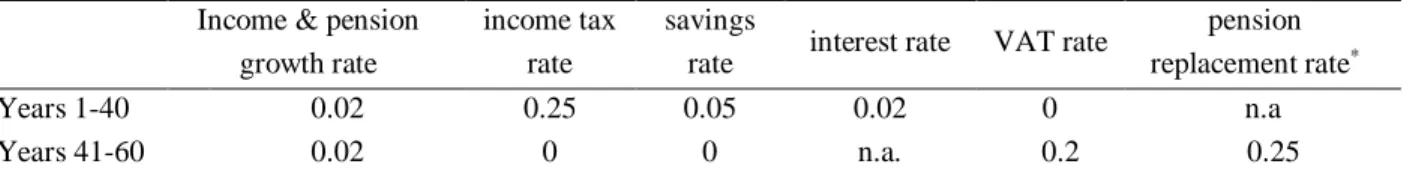
A Consumption Tax such as VAT (GST) is a Tax on Labour Income and Wealth In most OECD countries, by far the lion’s share of tax revenue is raised from taxes on income
For example, it is widely recognized that personal income tax rates can influence labor supply decisions, but the same potential responses apply to consumption taxes such as VAT.59. Their total retirement savings – representing the capital value of a potential pension – is part of their net worth and is naturally affected by the amount of income tax paid during their working life. Now consider the effect of the government introducing a 20% VAT from year 41 (income tax may be cut to compensate, but this has no effect on the pensioner whose only income, other.
This amounts to an additional tax liability on the retiree's accumulated wealth (and non-retirement expenses) of about $300,000 over 20 years of retirement on top of the $1.54 million paid in income tax during their working life.
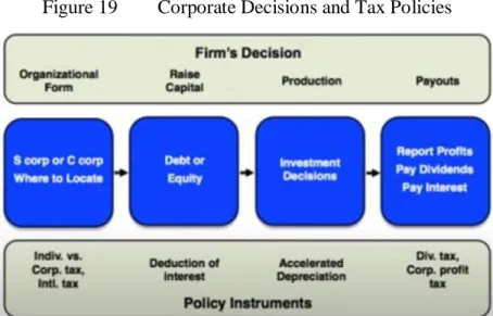
Both Statutory and Effective Tax Rates can be Relevant for Policy
Corporate income tax is a good example of the various decisions where statutory, effective marginal and effective average tax rates can each be relevant. 62 In much of the corporate tax literature, the terms “effective” and “marginal” or “average” are reversed in the tax rate definition, so that, for example, “EMTR” (EATR) becomes “METR” (AETR). Relevant analyzes often depend, among other things, on the precise form of the corporate tax regime.
Another example of the importance of different tax rates to address different tax policy questions is provided by Raj Chetty in the context of the American corporate tax regime.66 Figure 19 shows how the relevant tax policy instrument differs according to the type of firm decision being analyzed.
Conclusions
Theory of Tax Reform and Indian Indirect Taxation. 2019) Estimating Taxable Income Elasticities and Adjustment Costs from Tax Kink Bunching: Evidence from Register Data for New Zealand. 2016) Short-run and long-run participation tax rates and their impact on labor supply. 2012) Formalizing Good Tax Policy Practice: The New Zealand Model. Working Papers in Public Finances, No. Wellington School of Business and Government, Victoria University of Wellington, New Zealand.
Norman Gemmell is Professor of Public Finance at the Wellington School of Business and Government, Victoria University of Wellington, New Zealand.
Working Papers in Public Finance