Frequency-tuned surfaces for passive control of wall-bounded turbulent flow - a resolvent analysis study

(1)

J. Fluid Mech.(2023),vol.959, A26, doi:10.1017/jfm.2023.149

Frequency-tuned surfaces for passive control of wall-bounded turbulent ﬂow – a resolvent

analysis study

Azadeh Jafari^1,†, Beverley J. McKeon²and Maziar Arjomandi¹

1School of Mechanical Engineering, University of Adelaide, Adelaide, SA 5005, Australia

2Graduate Aerospace Laboratories, California Institute of Technology, 1200 East California Boulevard, Pasadena, CA 91125, USA

(Received 16 September 2022; revised 17 January 2023; accepted 16 February 2023)

The potential of frequency-tuned surfaces as a passive control strategy for reducing drag in wall-bounded turbulent flows is investigated using resolvent analysis. These surfaces are considered to have geometries with impedances that permit transpiration and/or slip at the wall in response to wall pressure and/or shear and are tuned to target the dynamically important structures of wall turbulence. It is shown that wall impedance can suppress the modes resembling the near-wall cycle and the very-large-scale motions and the Reynolds stress contribution of these modes. Suppression of the near-wall cycle requires a more reactive impedance. In addition to these dynamically important modes, the effect of wall impedance across the spectral space is analysed by considering varying mode speeds and wavelengths. It is shown that the materials designed for suppression of the near-wall modes lead to gain reduction over a wide range across the spectral space. Furthermore, a wall with only shear-driven impedance is found to suppress turbulent structures over a wider range in spectral space, leading to an overall turbulent drag reduction. Most importantly, the present analysis shows that the drag-reducing impedance is non-unique and the control performance is not sensitive to variations of the surface impedance within a favourable range. This implies that specific frequency bandwidths can be targeted with periodic material design.

Key words:drag reduction

† Email address for correspondence:[email protected]

licenses/by/4.0/), which permits unrestricted re-use, distribution and reproduction, provided the

original article is properly cited. 959A26-1

Published online by Cambridge University Press

(2)

1. Introduction

Turbulent skin-friction drag is a major constituent of the total drag in many engineering applications including air, sea, ground and fluid transportation. As an example, approximately half of the total drag on an aircraft is due to skin-friction drag (Gad-el-Hak 1994). Hence, due to the significant economic and environmental benefits, reducing skin friction has motivated considerable effort for the control of wall-bounded turbulence, including active and passive control techniques. A particularly attractive passive control concept, requiring no energy input and no complex control algorithms, is taking benefit of the wall material properties through the interaction between the wall and the turbulent flow, examples of which include perforated (Silvestriet al.2017; Bhatet al.2021; Jafari, Cazzolato & Arjomandi 2022), permeable (Breugem, Boersma & Uittenbogaard 2006;

Kuwata & Suga 2017; Suga et al. 2018; Chavarin et al. 2020, 2021) and compliant walls (Lee, Fisher & Schwarz1993; Xu, Rempfer & Lumley2003; Kim & Choi 2014;

Xia, Huang & Xu 2017). Based on the surface properties, these walls may suppress and/or energise specific frequency bandwidths within the turbulent flow. While some of the previous studies on permeable and compliant walls showed promising results, drag increasing cases, arising from energised large-scale spanwise structures (Jiménezet al.

2001; Breugemet al.2006; Kim & Choi2014; Luhar, Sharma & McKeon2015; Kuwata

& Suga 2017), were also found. The motivation of this study is to explore walls that could be tuned to passively suppress the dynamically important energetic structures of wall turbulence without significantly amplifying other scales, such that these frequency-tuned walls could create an overall reduction in drag.

We consider a general framework in which walls are designed with geometries that permit transpiration and/or slip in response to wall pressure and/or shear, and thus passively interact with the turbulent flow. We seek to determine the potential of such passive walls for reducing turbulent drag, thus shedding light on future surface designs.

In the present study, surface impedance is employed to describe the interaction of the frequency-tuned walls with the turbulent flow in terms of a modified wall-boundary condition, i.e. an impedance wall formulation. The surface impedance is commonly used as an effective boundary condition for acoustic analysis of the interactions of a surface with an acoustic field. In classical definitions, surface impedance defines a linear relationship between pressure and the flow velocity normal to the surface, i.e. a pressure-driven impedance. The classical pressure-driven impedance has been used in the literature, in the form of coupled wall-normal and pressure boundary conditions, for modelling of the boundary layer stability and transition over perforated surfaces (Burden1969; Porter 1998; Luharet al.2015). While the classical impedance formulation in previous studies correlates the wall-normal velocity and pressure at the wall, it does not account for the presence of viscous flow over the surface. It has been shown in the impedance eduction measurements in the presence of grazing flow (Renou & Aurégan2011; Dai & Auregan 2016; Boden et al.2017) that surface impedance is also correlated with the wall shear.

Hence, the effect of surface impedance on the turbulent flow can only be fully described if its correlation with wall shear, i.e. wall-shear-driven impedance, is also considered. This is also of significance for design of control strategies as the studies in the literature suggest a potential for passive control driven by wall shear. For example, Fukagataet al.(2008) showed that a compliant wall which could be deformed by both streamwise wall shear stress and pressure could create up to 8 % drag reduction in a turbulent channel flow.

Investigating the application of a wall-shear-driven compliant surface with in-plane wall deformations, Józsaet al.(2019) also found that passive streamwise in-plane motions of the wall could create up to 3.8 % drag reduction (Re_τ =180), while passive spanwise wall 959A26-2

(3)

fluctuations increased skin friction by more than 50 %. To our knowledge, despite previous studies on pressure-driven passive control, specifically passive walls such as permeable and compliant walls, a generalised theoretical model for pressure/shear-driven impedance walls is lacking.

This study develops a theoretical framework to investigate the interaction between the frequency-tuned walls and turbulent flows incorporating both pressure- and wall-shear-driven impedance. This framework is particularly beneficial for design of passive frequency-tuned walls and provides an understanding of the combined effects of passive pressure-driven and wall-shear-driven control approaches. Furthermore, this bulk approach based on surface impedance permits modelling of a surface with a general geometry without the need to resolve geometric details. The latter not only requires large and strenuous computations, but is also limited to the specific geometries considered.

Therefore, using the surface impedance formulation is advantageous for conducting a generalised and thorough analysis of the application of the described walls as a passive control strategy. As the classical impedance formulation only considers pressure-driven control, an improved generalised impedance formulation developed by Gabard (2020) is adopted in the present study. The generalised impedance defines a linear correlation between surface traction and flow velocity including the effects of mean shear at the surface (Gabard 2020), therefore incorporating both pressure- and wall-shear-driven control schemes into the impedance tensor and considering a surface that allows either or both transpiration and slip at the wall. This impedance formulation is introduced to the resolvent analysis formulation of McKeon & Sharma (2010) to investigate the effect of frequency-tuned surfaces on wall turbulence in the present study. By considering both wall-shear- and pressure-driven impedance components, the developed framework provides an improvement to the previous reduced-order models and can benefit design of passive flow control strategies.

The remainder of this paper is organised as follows. The resolvent analysis and impedance formulations are presented in §2. Section 3 describes the effect of wall impedance on modes throughout the spectral space, including those resembling the near-wall cycle (as categorised by Smits, McKeon & Marusic2011) and very-large-scale motions (VLSMs), with a streamwise length scale of λx>5–10δ that appear in the logarithmic region of the turbulent boundary layer at high Reynolds numbers and have a modulating effect on smaller-scale turbulent activity (Mathis, Hutchins & Marusic2009;

Smits et al. 2011). Section 4 compares control approaches based on shear-driven and pressure-driven impedances, and the effect of Reynolds numbers on the results is discussed in §5. Further discussions on design of frequency-tuned surfaces are presented in §6.

Finally, conclusions are drawn in §7.

2. Methodology

This section describes the modelling approach implemented for investigation of the effect of frequency-tuned surfaces on a fully developed turbulent channel flow. The frequency-tuned surface is introduced via an impedance formulation for the boundary conditions for the Navier–Stokes equations (NSEs). The induced change in the turbulent flow structure is analysed through the resulting change in the structure and amplification of the resolvent modes determined from resolvent analysis which are compared with the modes of the uncontrolled flow (a smooth impermeable wall). An overview of the resolvent formulation is provided in §2.1, and the impedance boundary condition accounting for the frequency-tuned surfaces is described in §2.2. The numerical implementation is described in §2.3, and finally verification of the conducted modelling is presented in §2.4.

959A26-3

(4)

2.1. Resolvent analysis

Resolvent analysis interprets the Fourier transformation of NSEs as a forcing-response system with feedback. In this formulation, the linear terms of the NSEs are driven by the feedback forcing, i.e. the nonlinear terms of the NSEs, to generate a velocity and pressure response. A low-order representation of the flow field is provided based on a gain-based decomposition of the forcing-response transfer function. This low-order formulation has been shown to reproduce the key structural features of wall turbulence (McKeon2017).

Specific resolvent modes have been associated with dynamically important structures of wall turbulence such as the near-wall cycle and VLSMs (Moarref et al. 2013; Sharma

& McKeon2013; McKeon 2017). It has been shown that these modes can be used as low-order models for assessment of control techniques (Luhar, Sharma & McKeon2014b;

Luharet al.2015; Nakashima, Fukagata & Luhar2017; Toedtli, Luhar & McKeon2019;

Chavarinet al.2021). The reader is referred to McKeon (2017) and Toedtliet al.(2019) for an in-depth discussion of the resolvent analysis and its application for evaluation of control techniques.

For a fully developed turbulent channel flow that is stationary in timetand homogenous in streamwisexand spanwisezdirections, the Fourier-transformed NSEs after Reynolds decomposition can be expressed as

uk

p_k

=

−iω I

0

−

Lk −∇k

∇^T_k 0

₋1

I

0

fk =Hkfk. (2.1) Here,u=[u, v,w]^T represents the streamwiseu, wall-normalvand spanwisewvelocity fields, andp is the pressure field.I andωare the identity matrix and angular frequency, respectively. Each wavenumber–frequency combinationk=(κx, κz, ω)represents a flow structure, or mode, with streamwise and spanwise wavelengths λx =2π/κx and λz= 2π/κz. These modes propagate downstream at streamwise wave speed c=ω/κx (the wave speed normalised with friction velocity isc⁺). Also,∇k =[iκx, ∂/∂y,iκz]^T and∇^T_k represent the gradient and divergence operators (whereT shows the transpose) andLk is the linear Navier–Stokes operator. As shown in (2.1), the resolvent operator,Hk, maps the nonlinear forcingf_k =(−u· ∇u)k to a velocity uk and pressure response p_k, where the Fourier coefficientuk andp_k denote the wall-normal variation in magnitude and phase of the velocity and pressure field for each modek. The special case ofk=(0,0,0)represents the mean velocity profileu0 =[U(y),0,0]^T. Note that all parameters are normalised with the friction velocity and half-channel height.

The resolvent operatorHk depends on the linear operatorLk, where Lk=

⎡

⎣−iκxU+Re⁻_τ¹∇_k² −∂U/∂y 0 0 −iκxU+Re⁻_τ¹∇_k² 0

0 0 −iκxU+Re⁻¹_τ ∇_k²

⎤

⎦. (2.2)

Here,Re_τ =u_τH/ν is the friction Reynolds number based on the half-channel heightH and∇_k²=[−κx²+∂²/∂y²−κz²] is the Fourier-transformed Laplacian.

A discretised singular value decomposition (SVD) of the resolvent operator yields a set of orthonormal forcing fk,m and response modes [uk,m,p_k_,_m]^T ordered based on the input–output gainσk,m. To ensure orthonormality of the resulting forcing and response modes under anL²energy norm, the resolvent operator of (2.1) is scaled such that

[Wu 0]

uk

p_k

=

[Wu 0]HkW⁻_f ¹

Wffk, (2.3)

959A26-4

(5)

or

Wuuk =Hk

SWffk. (2.4)

Here,Hk

Sis the scaled resolvent operator;WuandWf are diagonal matrices containing numerical quadrature weights, which ensure that the SVD of the resolvent operator,

Hk

S =

m

ψk,mσk,mφ^∗k,m (2.5) yields forcing modes fk,m=W⁻_f ¹φk,m and velocity response modes uk,m=W⁻_u¹ψk,m

with unit energy over the channel cross-section. Hence, (2.1)–(2.5) show that forcing in the direction of the mth singular forcing mode with unit amplitude fk,m creates a response in the direction of the mth singular response mode amplified by the singular value, i.e.σk,m[uk,m,p_k_,_m].

As shown by McKeon & Sharma (2010), the forcing-response transfer function tends to be low rank at the wavenumber–frequency combinations associated with the energetic structures in wall turbulence. Since a rank-1 approximation of the resolvent operator Hk

S≈ψk,1σk,1φ_k^∗_,₁is shown to represent the characteristics of the most energetic modes of wall-bounded turbulence (Moarref et al.2013), the rank-1 approximation is retained for the remainder of this study (refer to the Appendix for justification of this assumption and analysis of higher ranks) and for convenience the subscript 1 is dropped. The rank-1 velocity and pressure fields will be referred to as the ‘resolvent modes’ and the rank-1 singular valueσk,1referred to as ‘amplification’ or ‘gain’ for the remainder of this article.

The effect of wall impedance on the turbulent flow will be described in terms of velocity and pressure response for singular modes of dynamic significance in wall turbulence. In the present approach, only the shape and amplification of resolvent modes determined from the SVD are analysed, which is equivalent to considering unit amplitude forcing for allk.

To evaluate the potential of frequency-tuned surfaces for the control of wall turbulence, their impact on the Reynolds stress generation is also investigated. As discussed by Luhar et al. (2015), a suppression in the generation of Reynolds stress can be achieved through: (a) a reduction in the magnitude of or a change in the form of the nonlinear forcing that leads to a reduction of the magnitude of velocity response, (b) a reduction in the forcing-response gain or (c) a change in mode structure leading to a reduction in the Reynolds stress contribution from highly amplified resolvent modes. The present analysis will identify the effectiveness of the frequency-tuned surfaces as a control scheme through mechanisms (b) and (c) on a linear mode-by-mode basis noting that mechanism (a) requires knowledge of the nonlinear interactions, via the weighting factors (McKeon, Sharma & Jacobi2013) or statistical estimation methods (Towne, Lozano-Durán & Yang 2019), which themselves require data from experiment or simulation. While a more complete model would require knowledge of the nonlinear interactions and the coupling between the resolvent modes, previous studies have shown that analysis of the resolvent modes alone can provide valuable insight into the turbulent flow structure and can approximate the response of the full nonlinear system to control. Despite the considered simplifications in the present approach, it can determine control-induced drag reduction in trends which agree with direct numerical simulation (DNS) results, as shown by Toedtli et al. (2019). In addition, the present approach based on the mode-by-mode analysis provides valuable knowledge for optimal design of surfaces that have specific spatial periodicity that is tuned to specific frequencies, i.e. frequency-tuned surfaces, and are not aimed for overall drag reduction. Hence, a pattern search is adopted in the present approach 959A26-5

(6)

to find the wall impedance which favourably affects the turbulent flow structures with a focus on suppression of the resolvent modes resembling the near-wall cycle and VLSMs.

Favourable is defined as: (a) a reduction in forcing-response amplification (σk) relative to the uncontrolled flow, and (b) a reduction in the channel-integrated Reynolds stress contribution from the resolvent mode (RS), defined as (Luharet al.2015)

RS_k = 2

0 σk²Re(u^∗_kvk)(y−1)dy. (2.6) The weighted channel-integrated Reynolds stress in (2.6) is proportional to the turbulent component of friction coefficient in the turbulent channel flow.

2.2. Impedance boundary condition

The frequency-tuned surface is modelled by a generalised complex impedance. We implement the generalised impedance proposed by Gabard (2020) that correlates the forces inserted onto the surface by the fluid to the velocity vector via Cauchy stresses. This generalised complex impedance is defined as

Z¯ =

Z¯_tt Z¯_tn Z¯_nt Z¯_nn

, (2.7)

and

Z¯. u¯_t

¯ u_n

=

− ¯τnt

¯ p− ¯τnn

. (2.8)

Here,¯ represents dimensional variables, t is a unit vector tangent to the surface and n is the wall-normal unit vector pointing into the surface; Z¯_nn represents the classical acoustic impedance known as the inverse of admittance, i.e.Z¯_nn correlates the pressure at the surface to wall-normal velocity and if Z¯_nt =0, then: Z¯_nn= ¯p/v¯. This form of complex impedance in combination with a dynamic boundary condition to account for wall movements was previously used by Luharet al.(2015) to simulate a compliant wall (note that the impedance surfaces in the current study do not allow any wall deformation or displacements). In (2.8),Z¯_ttincorporates the effect of streamwise wall shear stress;Z¯_tn andZ¯_ntare related to the tangential force generated by the wall-normal velocity component and the normal force created by the streamwise velocity component, respectively. The non-diagonal components of the impedance tensor will be non-zero as, for instance for a perforated surface with the perforations made at an angle to the wall normal (Gabard 2020).

We apply the concept of generalised impedance for modelling the frequency-tuned surfaces and consider that the surface impedance affects the forces inserted on the flow at the wall boundary by permitting slip and/or transpiration. The effect of surface impedance is introduced as boundary conditions relating the fluctuating pressure and streamwise wall shear stress to the fluctuating streamwise and wall-normal velocities. Hence, the impedance boundary conditions at the bottom wall (y=0) are expressed as

−Z_xxu_k(0)+Z_xyvk(0)= 1 Re_τ

∂u

∂y(0), (2.9)

Z_yxu_k(0)−Z_yyvk(0)=p_k(0). (2.10) Note that here the wall-normal vector (yaxis) is pointing outward of the wall and all parameters are normalised with friction velocity (specificallyZ =Z¯/ρu_τ). We define the 959A26-6

(7)

boundary conditions such that a passive surface with a positive solely real Z_yy allows transpiration into the wall at high pressure regions. Accordingly, it is ensured that the wall surface receives more energy than it provides to the fluid. Similarly, a passive surface with a positive solely real Z_xx is defined to allow a negative slip velocity when at high shear stresses. Equations (2.9) and (2.10) together with the no-slip condition for the spanwise velocity (w_k =0) are applied within the resolvent before computing the SVD to introduce the effect of the frequency-tuned surface at the bottom wall.

At the top wall (y=2), the boundary conditions are expressed with a sign change to account for the change of wall-normal direction opposite to the channel y axis, and are given as

−Z_xxu_k(2)−Z_xyvk(2)= − 1 Re_τ

∂u

∂y(2), (2.11)

Z_yxu_k(2)+Z_yyvk(2)=p_k(2). (2.12) As described in §2.1, to determine the effect of surface impedance, the resolvent modes for the channel with impedance boundary conditions are compared with the uncontrolled flow with the standard no-slip boundary conditions (uk =vk=w_k =0) at the lower and upper walls.

2.3. Numerical implementation

A MATLAB code based on the resolvent code of a turbulent channel flow by Toedtliet al.

(2019) is developed and employed in the present study. The resolvent operator is discretised in the wall-normal direction (y) using a spectral collocation method on Chebyshev points.

The mean velocity profile U(y)needed for the resolvent operator is computed from the eddy viscosity model given by Reynolds & Tiederman (1967). It is assumed that the surface impedance does not alter the mean velocity profile and the same mean profile is applied to the case of the frequency-tuned surface. As discussed by Toedtliet al.(2019), a sufficient estimation for the response of the nonlinear system to control can be obtained by using the canonical mean velocity profile.

For the present study, a grid resolution study was conducted which showed that for N400, the singular values converged to within O(10⁻⁷) and O(10⁻⁴) for the uncontrolled and controlled flow cases, respectively. Similarly, the Reynolds stress contribution, RS_k, was found to converge to within O(10⁻⁴) for N 400 for both uncontrolled and controlled cases. Therefore, N=400 was used in this study, and N=800 was used only for the plots showing the wall-normal profiles (such asfigure 9).

2.4. Modelling verification and comparison with previous simulations

In order to verify the predictions of resolvent analysis with the impedance boundary conditions, the developed model is used for estimation of flow response to compliant and porous walls, and the results are compared with DNS results from three different studies.

It is important to note that the current model does not reproduce the entire flow field and the results are presented for one (or individual) resolvent modes. The model does not consider the feedback to the mean flow and assumes broadband forcing. In addition, the impedance formulation does not consider movement of the interface between the flow and the subsurface as opposed to the compliant walls in DNS simulations that move and deform. Considering these differences between the resolvent modelling approach and DNSs, lack of quantitative agreement and precise match of profiles is to be expected.

959A26-7

(8)

0.2 0.4 0.6 0.8 –(uv)

0 25 50 75 100 125 150 175 200

y⁺

0 2 4

σ² Re(u^∗v) 0

10 20 30 40 50 60 70 80

10^–2 10⁰ 10²

Nondimensional damping 0.5

0.6 0.7 0.8 0.9 1.0

Drag ratio

(a) (b) (c)

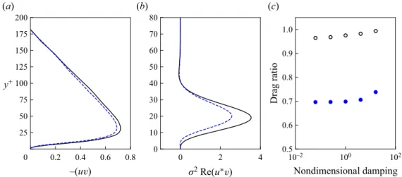
Figure 1. Resolvent analysis predictions for the passive streamwise-shear-driven impedance study by Józsa et al.(2019): (a) Reynolds shear stress profiles from DNS results by Józsaet al.(2019), and (b) Reynolds shear stress contribution of the resolvent mode representing the near-wall cycle. The black solid lines show the base flow and the dashed blue lines correspond to the control case. (c) The ratio of drag for control to base flow for different damping ratios obtained for the near-wall resolvent mode in comparison with total drag determined from DNS. The filled blue circles show the predictions by resolvent analysis and the unfilled black circles show the DNS results by Józsaet al.(2019).

However, it is demonstrated that the developed model is able to predict the impacts of surface porosity and compliance on the key structural features of turbulence (in terms of variations in resolvent modes).

First, a passive compliant wall driven by streamwise shear (Józsa et al. 2019) is considered. As found by the DNS of Józsaet al.(2019), a passive shear-driven compliant wall control reduces Reynolds shear stress specifically at its peak which is associated with the near-wall cycle (figure 1a). We employ resolvent analysis to evaluate the effect of the compliant wall by focusing only on the resolvent mode representing the near-wall cycle using a surface impedance tensor. For this compliant wall, Z_yy=Z_yx=Z_xy=0 andZ_xx is calculated using a mass–spring–damper model. The wall properties are used to calculate its mechanical admittance c_p =iω/(ω²Λm+iωΛd−Λs) (Landahl 1962) withΛm,Λd andΛsrepresenting the normalised mass, damping and spring coefficients (which as shown by Nagy & Paál (2019) can also be applied for shear-driven impedance).

This mechanical admittance is correlated to the normalised impedance as:Z_xx=1/Re_τc_p. For the compliant wall of Józsaet al.(2019), the mass, damping and spring coefficients normalised by the bulk channel velocity wereΛm=4,Λ_d =1 andΛs=0.5, which when normalised by friction velocity translate intoΛm=0.252,Λd=0.063 andΛs=0.0315.

Using these values atRe_τ =180 and for the resolvent mode representing the near-wall cycle(κx, κz,c⁺)=(1,11,10), it is found thatZ_xx= −0.0004+0.014i (with a negative sign applied to account for conversion of coordinates).

Figure 1(b) presents the predictions of resolvent analysis forZ_xx= −0.0004+0.014i on the turbulent Reynolds shear stress of the near-wall resolvent mode, andfigure 1(c) shows the effect of the damping of the passive wall on drag reduction (in terms of ratio of drag of the controlled flow to drag of base flow which for the model is calculated from (2.6)). Note that we are comparing results predicted by resolvent analysis for a single resolvent mode (the near-wall mode) with the full DNS results. While the Reynolds shear stress profile (of base and controlled flows) and the drag reductions do not describe the full flow, it is shown 959A26-8

(9)

2 4 6 8 10 k_x

4 6 8 10 12 14

c⁺

2 4 6 8 10

k_x 4

6 8 10 12 14

10⁰ 10¹

(a) (b)

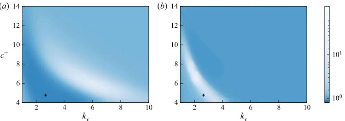
Figure 2. Gain ratios for spanwise-constant modes (κz=0) over a range of streamwise wavenumbers and wave speeds for the passive pressure-driven compliant wall by Kim & Choi (2014) predicted by resolvent analysis:

(a) considering only the wall impedance, and (b) considering both impedance and the wall motion. The+ symbol represents the two-dimensional waves observed in DNS of Kim & Choi (2014).

that the model is able to predict the response of the flow to shear-driven control and drag reduction in trends that agree with DNS results.

The second comparison is made for a pressure-driven compliant wall simulated by Kim & Choi (2014), in which large-amplitude two-dimensional waves were found to emerge. To model this compliant wall (case II in the study of Kim & Choi 2014), we determineZ_yyfrom the mechanical admittance formulation using the mass–spring–damper model (Zyy=1/c_p) and Z_xx=Z_xy=Z_yx=0. Here, as given by Kim & Choi (2014), Λm=2 and the spring and damper coefficients normalised with the bulk velocity are 1 and 0.5, which translate into 440 and 10.5, respectively, when normalised with friction velocity.Figure 2shows the gain ratios of two-dimensional resolvent modes (κz=0) over a range of streamwise wavenumbers,κx, and wave speeds,c⁺for this wall impedance at Re_τ =140. Gain ratio is defined as the ratio of singular value of the compliant wall to the base flow for each mode. As shown in figure 2(a), the predictions of the resolvent analysis show a region of high amplification at(κx,c⁺)≈(4.5,6.5)to(κx,c⁺)≈(8,5). However, these modes correspond to a larger streamwise wavelength compared with that found in the DNS results withλx =2.4h(κx =2.6). The main reason for this difference is lack of wall movement in the current model. This is demonstrated in figure 2(b), in which, in addition to the impedance boundary condition, wall movement is incorporated in the boundary conditions using a linearised approximation by the equation derived by Luhar et al. (2015) (vk(0)= −iωηk, where ηk is the Fourier coefficient for wall displacement). With consideration of wall movement, the amplified modes correspond closely to those predicted in the DNS study. This comparison also suggests that the deteriorating mechanisms observed over compliant walls are closely correlated with the wall movement.

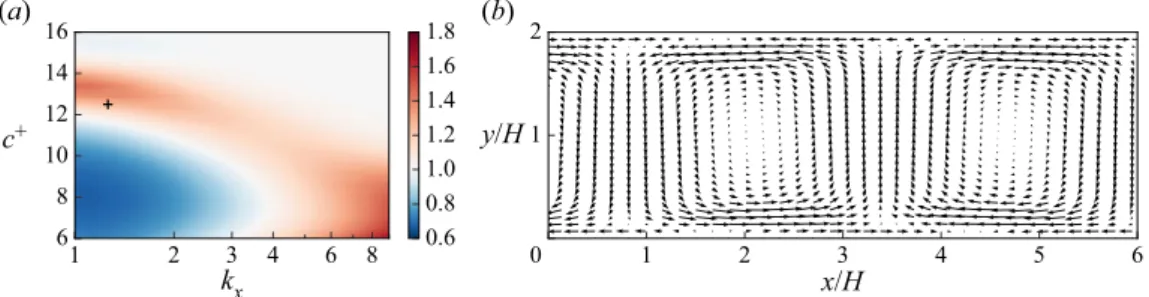
Finally, an analogy between surface impedance and permeability is adopted and the resolvent predictions are compared with the results of a previous DNS study of a zero-pressure-gradient boundary layer over a Darcy-type porous wall (Jiménez et al.

2001). Surface permeability,K, is interpreted as the inverse of pressure-driven impedance resistance, i.e. Re(Z_yy), and for a surface withZ_yy=K⁻¹ (noting that permeability can be interpreted as a time-averaged impedance). The developed model is used to predict the two-dimensional resolvent modes (κz=0) for a wall with Z_yy=18.52 (and Z_xy= Z_yx=Z_xx=0) representing the porous wall of Jiménezet al.(2001). Figure 3(a) shows the ratio of singular values for the porous wall over an impermeable wall (base flow) at 959A26-9

(10)

1 2 3 4 6 8 k_x

6 8 10 12 14 16

c⁺

1 2 3 4 5 6

x/H 0

1 2

y/H

0.6 0.8 1.0 1.2 1.4 1.6

(a) 1.8 (b)

Figure 3. Resolvent analysis predictions for the porous wall of Jiménezet al.(2001): (a) ratio of porous to impermeable wall singular valuesσkc/σk0for spanwise-constant resolvent modes for a range of streamwise wavenumbers and wave speeds atRe_τ =180; (b) wall-normal and streamwise velocity fields for the amplified mode at(κx, κz,c⁺)≈(1.2,0,12.5). The + symbol in (a) shows the wavenumber and speed of rollers identified in the DNS study by Jiménezet al.(2001).

Re_τ =180.Figure 3(a) shows a region of high amplification between(κx,c⁺)≈(1,12) and(κx,c⁺)≈(2,14), with singular value ratios of≈1.6. The wavelength at this peak region corresponds closely to the spanwise rollers identified by Jiménezet al.(2001) which were found to emerge over the porous wall with a wavelength ofλx/H=5 propagating downstream at a speed ofc⁺=12.5 (shown by the+symbol infigure 3a).Figure 3(b) shows the streamwise wall-normal velocity field for this amplified mode over the porous wall. The counter rotating spanwise rollers which represent those observed in the DNS study (figure 7 in Jiménezet al.2001) are clearly identified. Hence, it is shown that the present analysis with the impedance formulation can predict amplification of the spanwise rollers over the porous wall, in agreement with the results of Jiménezet al.(2001).

3. Results

The effectiveness of frequency-tuned walls as a control method is evaluated through analysis of its impact on the near-wall cycle and VLSMs in §§3.1and3.2. As discussed in the literature (Luharet al.2014b,2015; Luhar, Sharma & McKeon2016), suppression of these modes is a starting point for achieving an effective control. In §3.3, the effect of surface impedance on other scales is considered. The results in this section are presented forRe_τ =2000, which is the lowest Reynolds number at which the VLSMs are known to become prominent (Smitset al. 2011). Note that we assume a general geometry that permits slip and transpiration as provided by the analysis

3.1. Effect of wall impedance on near-wall modes

In this section, the modes resembling the near-wall cycle corresponding to k= (κx, κz,c⁺)=(12,±120,10) are considered. This wavenumber–speed combination at Re_τ =2000 corresponds to λ⁺x =2πRe_τ/κx ≈10³ and λ⁺z =2πRe_τ/κz≈10², which represent the near-wall cycle (McKeon & Sharma2010). First, diagonal impedance tensors (Z_xy=Z_yx=0) are considered and a pattern search is conducted to find impedance values (Zxx and Z_yy) that lead to a reduction of mode gain and Reynolds shear stress contribution.Figure 4shows the ratios of controlled to uncontrolled mode gain,σkc/σk0, and channel-integrated Reynolds stress contribution,RS_kc/RS_k0, for a range of Z_xx and Z_yyvalues. First, sweeps over individual parameters (only non-zeroZ_xxand only non-zero Z_yy) are conducted and next bothZ_xxand Z_yyare varied. The blue regions in the figures 959A26-10

(11)

10⁰ 10¹ Re(Z_xx)

10^–1 10⁰ 10¹

Im(Zxx)

1

10⁰ 10¹

Re(Z_xx) 10^–1

10⁰ 10¹

Im(Zxx)

1

0.8 0.9 1.0 σkc/σk0

0 0.4 0.8 1.2 RS_kc/RS_k0

10⁰ 10¹

Re(Z_yy) 10^–1

10⁰ 10¹

Im(Zyy)

1

10⁰ 10¹

Re(Z_yy) 10^–1

10⁰ 10¹

Im(Zyy) ¹

0.6 1.0 2.0 5.0 8.0 σkc/σk0

0.01 0.10 1.00 10.00 50.00 RS_kc/RS_k0

10⁰ 10¹

Re(Z_xx) 10^–1

10⁰ 10¹

Im(Zxx)

1

10⁰ 10¹

Re(Z_yy) 10^–1

10⁰ 10¹

Im(Zyy)

1

0 1 2 3 4 RS_kc/RS_k0

0.1 1.0 10.0 100.0 RS_kc/RS_k0

(a) (b)

(c) (d)

(e) (f)

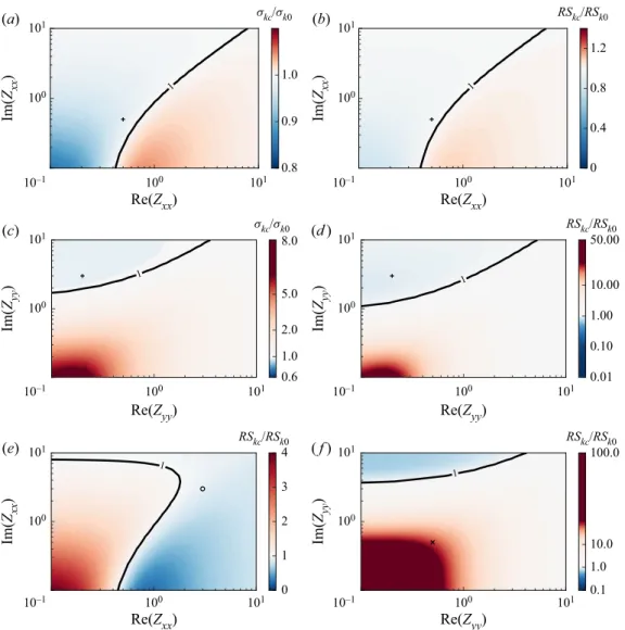
Figure 4. Contour maps showing the ratio of control to uncontrolled flow singular values σkc/σk0 and channel-integrated Reynolds stressRSkc/RSk0for the resolvent modes resembling the near-wall cycle over a range ofZxxandZyyvalues for a diagonal impedance tensor (Zxy=Zyx=0). (a,b) Ratios of singular value and Reynolds stress for a sweep overZxxatZyy=0, (c,d) ratios of singular value and Reynolds stress for a sweep overZyyatZxx=0, (e) Reynolds stress ratios for a sweep overZxxatZyy=0.2+3i (the+symbol inc,d) and (f) Reynolds stress ratios for a sweep overZ_yyatZ_xx=0.5+0.5i (the+symbol ina,b). The◦and×symbols in (e,f) show the favourable and unfavourable cases referred to infigure 5.

show the Z_xx and Z_yy values which reduce the amplification and Reynolds shear stress contribution compared with the uncontrolled flow and suppress the near-wall mode.

Figure 4(a,b) shows the effect ofZ_xx on the near-wall mode consideringZ_yy=0, i.e.

a wall that permits only slip and no transpiration. It is found that this impedance can weaken the near-wall mode mainly for Z_xx values with a larger imaginary component (more reactive than resistive) especially for Re(Z_xx) <1. A solely realZ_xx will amplify the near-wall mode and increase its Reynolds shear stress if Re(Z_xx) >0.4. The largest reductions in amplification and Reynolds stress contribution, 15 % and 23 %, are achieved for Re(Z_xx)≈Im(Z_xx) <0.2.Figure 4(c,d) shows the effect ofZ_yyon the near-wall mode 959A26-11

(12)

consideringZ_xx=0, i.e. a wall that permits only transpiration. Here, cases with Re(Z_yy)≈ Im(Z_yy)≈0.1 significantly amplify the resolvent mode and increase its Reynolds stress contribution. OnlyZ_yyvalues with a larger imaginary component (Im(Z_yy) >2) suppress the near-wall mode. The largest reductions in mode gain and Reynolds shear stress contribution of the resolvent mode are 5 % and 15 %, which are almost insensitive to the value of Z_yy in its favourable range (the blue zone in figure 4c,d). The combined effects of bothZ_xx andZ_yyare considered infigure 4(e,f) in which, for brevity, only the channel-integrated Reynolds shear stress is shown.Figure 4(e) shows a sweep over Z_xx for a constantZ_yy =0.2+3i, which, as shown in panels (c,d), is favourable in terms of suppression of the near-wall resolvent mode. Similarly, figure 4(f) shows a sweep over Z_yy forZ_xx=0.5+0.5i. In both cases, combinations ofZ_xx and Z_yy exist that suppress the near-wall mode and reduce its Reynolds stress contribution. The results show that the favourable range ofZ_xxis changed whenZ_yy is non-zero. As shown infigure 4(a), for a purely shear-driven impedance, a more reactiveZ_xxsuppresses the near-wall mode, while for combined pressure- and shear-driven impedance,figure 4(e), the effective angle ofZ_xx is different. However, as shown in figure 4(d,f), the effective angle of Z_yy is the same for a zero and a non-zeroZ_xx. The pattern searches are conducted for other values ofZ_xx andZ_yy and it is found that, in general, the limiting factor in reduction of mode gain and Reynolds shear stress isZ_yy, which suppresses the near-wall mode for values with larger imaginary components while a purely realZ_yyis mostly unfavourable and increasesRS_kc (similar to the observations infigure 4d,f). Furthermore, as shown in the contour maps, for favourable ranges ofZ_xxandZ_yy,σkc/σk0andRS_kc/RS_k0remain almost constant and the flow response becomes insensitive to the impedance values. This suggests that, with the increase of surface impedance, the resulting dynamics overwhelms the dynamics of the uncontrolled near-wall mode.

Based on the trends observed infigure 4, two cases of favourable and unfavourable wall impedance are selected and the effect of wall impedance on mode structure is discussed.

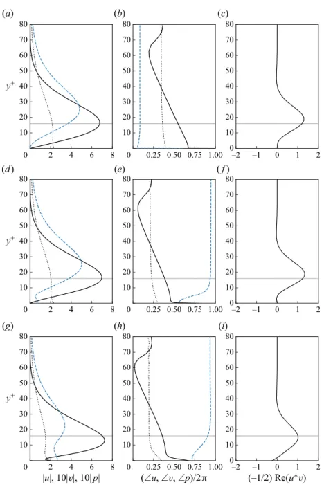
Figure 5 shows the wall-normal profiles of the velocity and pressure fields and the normalised Reynolds stress contribution of the resolvent mode resembling the near-wall cycle for the uncontrolled and controlled flows with favourable and unfavourable wall impedance tensors. For the uncontrolled case, the resolvent mode structure is consistent with the previous studies (McKeon & Sharma2010; Luharet al.2014b,2015), where the streamwise velocity reaches its peak at the critical layer,y⁺_c (the wall-normal height where the mode speed is equal to the mean velocity), and the wall-normal velocity peaks further away from the wall. The streamwise and wall-normal velocities for this mode have a phase difference of≈πaty⁺_c resulting in the peak of Reynolds stress contribution at the critical layer. The wall-normal and pressure fields maintain a constant phase withyand a constant phase difference of≈π/2.

For the favourable wall impedance,figure 5(d–f), the wall-normal velocity is modified substantially compared with the uncontrolled case, having a non-zero and constant magnitude near the wall,y⁺<5, i.e. wall transpiration (note that it is assumed that the wall can support the given impedance with a geometry that can support transpiration and/or slip). The phase of wall-normal velocity is no longer constant below the critical layer approaching the wall. Hence, the phase difference between wall-normal velocity and pressure fields is reduced near the wall. Also, the phase difference between streamwise and wall-normal velocity fields is reduced near the wall below the critical layer. These changes yield a modification in the Reynolds shear stress distribution at the proximity of the wall.

The peak of Reynolds shear stress remains almost consistent with the uncontrolled case.

However, the Reynolds shear stress contribution of this mode is reduced significantly 959A26-12

(13)

2 4 6 8 0

10 20 30 40 50 60 70 80

y⁺

0.25 0.50 0.75 1.00 0

10 20 30 40 50 60 70 80

–2 –1 0 1 2

0 10 20 30 40 50 60 70 80

2 4 6 8

0 10 20 30 40 50 60 70 80

y⁺

0.25 0.50 0.75 1.00 0

10 20 30 40 50 60 70 80

–2 –1 0 1 2

0 10 20 30 40 50 60 70 80

2 4 6 8

|u|, 10|v|, 10|p|

0 10 20 30 40 50 60 70 80

y⁺

0.25 0.50 0.75 1.00 (∠u, ∠v, ∠p)/2π 0

10 20 30 40 50 60 70 80

–2 –1 0 1 2

0 10 20 30 40 50 60 70 80

(–1/2) Re(u^∗v)

(a) (b) (c)

(g) (h) (i)

(d) (e) (f)

Figure 5. Profiles showing the wall-normal variation in structure for the resolvent mode resembling the near-wall cycle: (a,d,g) amplitude and (b,e,h) phase for the streamwise velocity (solid lines), wall-normal velocity (dashed lines) and pressure fields (dotted lines); (c,f,i) the normalised Reynolds stress contribution.

(a–c) Represent the uncontrolled flow (the impermeable wall), (d–f) represent a favourable wall impedance (Zxx=3+3i, Zyy=0.2+3i, Zxy=Zyx=0) and (g–i) represent an unfavourable wall impedance (Zxx= 0.5+0.5i,Zyy=0.5+0.5i,Zxy=Zyx=0). The dotted horizontal lines show the location of the critical layer for this resolvent mode aty⁺≈15.

due to the reduction of the mode amplification (since it is proportional to σ_k² as given in (2.6)). The main drag reduction mechanism here therefore is suppression of the mode and reduction of the mode gain.

959A26-13

(14)

10⁰ 10¹ Re(Z_xy)

10^–1 10⁰ 10¹

Im(Zxy) Im(Zyx)

1

10⁰ 10¹

Re(Z_yx) 10^–1

10⁰ 10¹

1

0.8 1.0 1.5 RS_kc/RS_k0

0.4 1.0 5.0 RS_kc/RS_k0

(a) (b)

Figure 6. Contour maps showing the ratio of control to uncontrolled flow channel-integrated Reynolds stress RSkc/RSk0for the resolvent modes resembling the near-wall cycle over a range of (a)Zxyvalues andZyx=0, and (b)Zyxvalues andZxy=0 for a favourable diagonal wall impedance (Zxx=3+3i,Zyy=0.2+3i). The +symbols show the favourable impedance values presented in parts (d) and (e) infigure 7, respectively.

For the unfavourable wall impedance,figure 5(g–i), the wall impedance yields large slip and transpiration velocities at the wall. The peak of the streamwise velocity is also shifted closer to the wall below the critical layer (y⁺<y⁺_c). Consequently, the peak of Reynolds stress is shifted slightly to below the critical layer. For this case, the phase difference between streamwise and wall-normal velocities is reduced below the critical layer which modifies the Reynolds shear stress near the wall.

After determination of the favourable and unfavourable ranges of the diagonal components of the impedance tensor, the gain and Reynolds stress contribution of the near-wall mode were calculated over a sweeping range of the non-diagonal components (positive values of Z_xy and Z_yx). Note that it is expected that the results will not change by sweeping over the non-diagonal components followed by sweeping over diagonal components as indicated from some trials. The results showed that, for the diagonal components,Z_xx and Z_yy, in the unfavourable ranges of figure 4, the near-wall mode remains unfavourable, insensitive to the variations of the non-diagonal impedance components. For a favourable diagonal impedance, the gain of near-wall mode was found to be insensitive toZ_xy, but there exists only a favourable range of Z_xy and Z_yx which reduce the Reynolds shear stress contribution of the near-wall mode.Figure 6(a,b) shows RS_kc/RS_k0for sweeps overZ_xyandZ_yx, respectively. Only values of Re(Z_xy)≈Im(Z_xy) <

2 reduce the channel-integrated Reynolds stress and large values of Z_xy increase the Reynolds stress contribution of this mode. As shown infigure 6(b), the channel-integrated Reynolds shear stress increases compared with the base flow for Re(Z_yx) <2 and 0.2<

Im(Z_yx) <3.

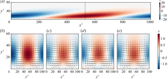
The effect of the non-diagonal components of the impedance tensor on the near-wall mode is further analysed by comparison of the predicted velocity fields with those of the uncontrolled flow for the resolvent mode resembling the near-wall cycle.Figure 7(a,b) shows the velocity fields of the near-wall mode for the uncontrolled flow in streamwise wall-normal(x–y)and spanwise wall-normal (z–y)planes. Note that the cross-sectional views in the(z–y)planes for all cases are shown at the location where the streamwise velocity magnitude is maximum, which for the uncontrolled flow is shown by the dashed line in figure 7(a). The counter rotating streamwise vortices and the periodic ejections and sweeps commonly associated with the near-wall cycle are clearly seen in figure 7(a,b). Figures 7(c)–7(e) show the velocity structure in the (z–y) plane for a favourable diagonal impedance tensor (Zxx=3+3i, Z_yy=0.2+3i shown by the 959A26-14