Modelling Wear Patterns on Footwear Outsoles

(1)

Modelling Wear Patterns on Footwear Outsoles

a dissertation presented by Xavier S. Francis

to

The School of Computing&Information Technology in partial fulfillment of the requirements

for the degree of Master of Computing Unitec Institute of Technology

Auckland, New Zealand may 2019

(2)

(3)

Modelling Wear Patterns on Footwear Outsoles

Advisors

Principal Associate Associate Dr Hamid Sharifzadeh Angus Newton Dr Nilufar Baghaei

Abstract

The outsoles of footwear develop nicks, cuts, and tears via repeated exposure to the abrasive forces that occur between the outsole and the ground. These abrasions result in the formation of characteristics unique to the outsole and the individual wearing them; additionally resulting in the degradation of the outsole design imprinted by the manufacturer. The combination of these characteristics allow the forensic scientist to uniquely identify the individual to whom it belongs. Quite often a period of time can elapse between the discovery of a shoeprint at the crime scene and the identification of a suspect. In these instances, the forensic scientist must rely on their training and expertise—developed through years of experience and study—to determine if the crime scene shoeprint matches the outsole of the suspect’s shoe.

This work introduces a computational framework capable of modelling wear patterns on the outsoles of footwear. This model is able to predict the evolution of the wear pattern after an arbitrary time period given in weeks. We introduce an additional model capable of reconstructing the outsole back to its original state on a given week. This framework—built on convolutional neural networks—

provides an objective point of reference for forensic scientists in their evaluation of outsole wear patterns.

(4)

Publications

Learning Wear Patterns on Footwear Outsoles Using Convolutional Neural Networks.

Accepted in theIEEE International Conference on Trust, Security and Privacy in Computing and Com- munications, Rotorua, New Zealand—by X. Francis, H. Sharifzadeh, A. Newton, N. Baghaei,&S.

Varastehpour (August 2019).

Feature Enhancement and Denoising of a Forensic Shoeprint Dataset for Tracking Wear- And-Tear Effects. Submitted to theIEEE Global Conference on Signal and Information Process- ing, Ottawa, Canada—by X. Francis, H. Sharifzadeh, A. Newton, N. Baghaei,&S. Varastehpour (November 2019).

Modelling Wear Patterns on Shoeprints Using End-To-End Deep Learning. Submitted to the IEEE Transactions on Pattern Analysis and Machine Intelligence—by X. Francis, H. Sharifzadeh, A.

Newton, N. Baghaei,&S. Varastehpour (May 2019).

(5)

Acknowledgements

To my advisor, Hamid—for his guidance, for his faith in my abilities, and for the opportunity to work on this project,

To my co-advisors, Angus and Nilufar—for their invaluable insights and assistance, To my parents, Mary and Francis—for their conviction that my education was their best investment, and

To all those who came before me—whatever their contributions to the field, great or small.

I stand on the shoulders of giants.

Thank you.

(8)

Introduction 0

Forensic science sees the application of scientific methods to aid in the practice of criminal investigations. The earliest applications of the field can be found as far back as the 13th century in China [1]. Practitioners—known as forensic scientists—collect, process, and analyse evidence and other materials found at the scene of a crime to aid in the criminal investigation. Over the years, forensic science has brought many other sciences into its fold to be applied to criminology; spawning nu- merous sub-disciplines that specialise in art, botany, chemistry, archaeology, accounting, digital forensics, and much more. With the human element, forensic scientists consider human behaviour and biometric signatures such as dna [2], hair [3], blood [4], fingerprints [5], etc.

Forensic podiatry is the sub-discipline that deals with the application of podiatric knowledge to crime scene investigations [6]. This practice aims to answer any questions regarding matters of the foot or footwear to forensic science and so studies aspects like bare footprints, footwear, and gait analysis. Some of the most common types of evidence found at crime scenes are marks and prints formed by the footwear worn by the criminal(s); their study being recorded as far back as 1786 [7]. These marks are imprints formed by the outside sole (outsole) of the footwear when it comes into contact with a surface. Imprints may be three-dimensional, when present in surfaces like sand or snow—or more commonly—two-dimensional impressions found on carpet, tiles, and other flooring. To capture shoeprint evidence, a cast is taken if the impression is in a 3-dimensional

(9)

setting, else an image is obtained through gel or photography. The image of the shoeprint is first digitally enhanced, removing noise and other artefacts of scanning; and then compared against a database of known prints and prints collected from other crime scenes to find a match [8]. Such shoeprints are capable of uniquely linking a suspect to a crime by the skilled forensic practitioner as they are as strong as other kinds of impression evidence like fingerprints [9]. They also serve to link different crime scenes of the same offender [10].

Despite their uniquely identifiable nature and the frequency of their discovery at crime scenes, shoeprints are not often used as evidence in a criminal trial, due to the variation in quality of scene- of-crime prints. Often, the retrieved crime scene print can be incomplete or degraded. A study out of the Netherlands found that in 1993, only 500 out of 14,000 shoeprints were positively identified [11]. The variations in quality can arise from the surface on which footwear pressure is applied, or from the walking patterns of the wearer. Nevertheless, shoeprint evidence have proven to be an effective method of linking suspects to crime scenes and the study of footwear has earned a place under the forensic science umbrella.

The characteristics that describe shoeprints are of two types.Class characteristicsare those features of a shoeprint that are capable of linking it to the manufacturer, brand, and model of the shoe [12]. They describe the geometric patterns of the outsole imprinted by the manufacturer for aes- thetic and practical purposes. Since there are a large number of shoe manufacturers, models, and designs, class characteristics serve to narrow down the search space to identify a given suspect’s shoeprint.Individualising characteristicsare those characteristics that arise on the outsole as a function of wear [13]. They consist of nicks, cuts, abrasions, punctures, tears, and other types of marks that form on the outsole as a result of the wearing process. The position, configuration, and orientation of each of these defects—combined—are capable of uniquely identifying the shoe on which they form. The position of a defect is its location relative to the perimeter, tread patterns and the like. Shapes are defined by width, height, and area. The rotation of a characteristic helps to separate it from other similarly shaped defects. The combination of class and individual characteristics are analysed by a shoeprint examiner to uniquely identify a suspect’s shoe and to attribute it to a crime scene shoeprint.

Thewear patternis the sum total of individualising characteristics present on the shoeprint. This is unique to an item of footwear and is formed by erosion of the outsole through repeated use. The environment the shoes are worn in, the height and weight of the person wearing them, the frequency and nature of use are all factors that influence wear. To analyse these wear patterns, forensic scientists rely on their knowledge and skills—gained through years of study and experience. Quite often a gap of weeks or months can elapse before a suspect is identified and his/her shoeprints are

(10)

obtained. Insights into how wear characteristics develop over time can help the forensic investigator develop a better ability to interpret them. Pattern recognition can be subjective and an experienced examiner may more accurately identify and assess patterns in evidence [14]; although attempts have been made to formalise their interpretation [15–18]. Computer aided identification and analysis can help alleviate inherent human biases as well as intra-analyst variation in identifying features or characteristics in the evidence by complementing the forensic examiner’s skillsets.

Due to the rate of outsole patterns being designed and manufactured, any archive of shoeprints will quickly go out of date, if not diligently maintained. This compounds the difficulty of identifying class characteristics of crime scene prints. To assist the forensic examiner in such tasks, computational methods have been developed, driven by the interdisciplinary field ofcomputational foren- sics—the application of computational models, analysis, algorithms, and simulations to assist in the identification and analysis of forensic evidence [19]. Earlier approaches relied upon statistical and mathematical methods to form quantitative analyses of evidence. Criticisms of forensic testimony for lacking a scientific basis—among other reasons—have led to the development of computer aided methods in assisting forensic investigations [20]. These methods can objectively analyse and identify the class characteristics of a given shoeprint, providing metadata—like make and model—

exponentially faster than an individual can look it up.

This thesis contributes to the literature by introducing a computational model and framework for studying and analysing wear patterns on footwear outsoles. We present a methodology that leverages deep neural networks (dnns) to model the wear pattern captured in a unique dataset of shoeprints. We hope that our models can serve as an empirical point of reference for the forensic science community; additionally providing a platform for novice forensic scientists to hone their skills with.

∗ ∗ ∗

The rest of this dissertation is organised as follows:

• In Chapter 1 we review the field of computational forensics; surveying the work in the domains of shoeprint classification and shoeprint wear, with a special focus on machine learning applications in the field.

• Chapter 2 introduces a unique dataset collected for the purpose of studying wear patterns.

We describe the challenges faced in preparing this dataset for predictive modelling and detail a novel denoising methodology that satisfies our unique constraints.

(11)

• Chapter 3 presents the core of the thesis—computational models of shoeprint wear. We describe the mathematical algorithms that power our methodology and introduce two models built using this method—the first capable of predicting wear patterns on outsoles and the second able to reconstruct the outsole to its original state.

• Finally, in Chapter 4, we summarise the ideas of the thesis and point to directions of future work.

(12)

Chance favors the prepared mind.

Louis Pasteur

Computational Forensics 1

The forensic examiner’s role in a criminal investigation is to identify, preserve, and analyse all evidence of crime in order to—(i) eliminate items that are not relevant to the investigation, (ii) identify evidence that may link a suspect to the crime, (iii) provide proof of an individual’s involvement in a crime, and (iv) to provide written reports or testimony as required.

The responsibilities of the forensicfootwearexaminer are—(i) to identify class characteristics of a given shoeprint, by comparing it against a large set of known prints to discover details like manufacturer, make, and model and (ii) to consider the individualising characteristics of the print to assign the print to an owner. The computational methods developed to assist the examiner in these tasks fall under three domains:

1. Shoeprint classification—systems that match class characteristics in a query image to those in a database of reference images,

2. Shoeprint wear—those studies that look at the formation of accidental characteristics on outsoles over a period of time, and

3. Machine learning—research that sees ml methodologies applied to the analysis of shoeprints.

(13)

1.1 Shoeprint classification

Researchers have to work with several challenges when designing systems of shoeprint recognition. High quality reference images found in reference databases are taken by the shoeprint examiner in laboratory conditions, while the query prints that need to be matched are scene-of-crime images (socs). Crime scene impressions are often incomplete, noisy, and/or distorted. Automated methods have to consider these variables to be a robust recognition system. At a high level, all the methods surveyed in this section follow a similar pattern—first a data pre-processing stage is conducted, where the input image is cleaned, denoised, and rotated, as required. Then key-points or featuresof the shoeprint are computed and compared against the same metric for each shoeprint in the database, in the hopes of finding a match for class characteristics. Over the years, shoeprint retrieval systems have developed more efficient ways of pre-processing, feature extraction, and similarity measurement. We begin by looking at classification methods that are partially automated.

1.1.1 Semi-automated methods

The earliest methods used a semi-automated approach and appeared in the mid 90s [21–23]. By manually encoding the obtained print and reference images using shape primitives (e.g. geometric shapes, patterns etc.), these systems were able to find a match [24,25]. These methods required significant manual intervention, were time-consuming in performance, and were prone to error be- cause different analysts may encode the primitives in different ways. The practice of shoeprint classification was new and immature, but early results instilled confidence that computational methods could prove effective in aiding the forensic examiner.

1.1.2 Automated methods

One of the earliest automatic methods was presented by Geradts and Keijzer [11] who developed a database of reference shoeprints (labeled ‘rebezo’), in addition to their proposed method which computed Fourier features of print segments and used an artificial neural network for classification. Alexander et al. [26] devised a method where shoeprint images are decomposed into fractals and the coefficients are matched against a database of prints. The fractal decomposition of a database image with minimal changes to the image under test is considered to be a match. Mean square noise error was used to compute this change. In later work [27], they test the system’s ro- bustness in dealing with rotation and translation.

de Chazal et al. [28] discussed a technique that used discrete Fourier transformations, and calculated the coefficient of power spectral density (psd). Pattern matching was done using 2d correlation coefficient similarity measure. Their tests showed the system returning a positive match

(14)

in the first result 65 percent of the time. However, their model works regardless of the spatial positioning of the print. Zhang and Allinson [29] represented shoeprint features using edge-direction histograms, and computed 1d discrete Fourier transforms on the normalised histogram. The similarity measure used was the Euclidean distance. Su et al. [30] introduce a method of thresholding shoeprint patterns in noisy images by extending a general model out of non-local mean filtering.

Pavlou and Allison [31] presented a technique that uses local image features, where maximally stable extremal region (mser) feature detectors are encoded using scale invariant feature transform (sift) descriptors to obtain a match, using a Gaussian weighted similarity metric. Pavlou and Allison on this work by encoding a codebook of histograms representations for each shoe pattern and clustering them using k-means to facilitate fast indexing [32]. Ghouti et al. [33] proposed using directional filter banks (dfbs) to create a condensed representation of a shoeprint they called

‘ShoeHash’. This method would encapsulate both local and global details of the print and used a normalised Euclidean distance to assess similarity. Su et al. [34] have utilised a hybrid pattern and topological spectra—using the Euler number—and computed similarity using the normalised value of these two measures. In Crookes et al. [35], the authors propose a feature detection method they call ‘enhanced local image feature’ which combines an automatic Laplace-based scale selection with the Harris corner detector. sift descriptors are used to represent features. They match two images based on their descriptors using a nearest-neighbour search.

Gueham et al. [36] evaluated an advanced correlation filter—otsdf—for classification. The method processes partials and distorted prints. They propose an alternate method [37] where feature extraction is done using the the Fourier-Mellin transform (which involves a log-polar mapping and a Fourier transform). They use a 2d correlation method to find similarities between shoeprints.

Their method was tested on a dataset including degraded images and proved to be efficient. In Al- Garni and Hamiane [38], Hu moment invariants are used to classify shoeprints. They opted to compute similarity with the most common distance measures seen in the literature—City-block, Euclidean, Canberra, and Correlation. The method performs perfectly with rotated images, and well with lower resolution images, but performance drops drastically on noisy query images. Xiao and She [39] further the work done with psd by pairing it with Zernike moments—the Zernike method being used to handle distorted prints, and the similarity measured by the correlation coefficient of psd.

Jing et al. [40] performed feature extraction based on the direction of patterns present in the print (vertical lines, circular shapes, geometries etc.). They capture patterns on three levels—using co-occurrence matrices, directional masks, and local and global Fourier transforms. Using these feature vectors, they compute a similarity using the sum-of-absolute-difference. In Nibouche et

(15)

al. [41], Harris points and sift descriptors are combined in a method of feature extraction. The method was compared to de Chazal et al. [28] and found to be superior. This method is designed to work with partials, and is rotation and noise resistant. Matches are found using the ransac algorithm.

Dardi et al. [42] noted that most of the literature that came before them were tested on arti- ficially generated crime scene prints, and developed a texture based method that computed the Mahalanobis distance for a print as the feature descriptor, which they tested on real crime scene prints. The authors go on to test this system in subsequent work [43,44], comparing the performance using synthetic and real crime-scene prints against de Chazal et al. [28] and Gueham et al.

[36]. Wang et al. [45] have used wavelets as an edge detector and neural networks for recognition.

In Patil and Kulkarni [46], shoeprint rotation estimation is handled using Radon transform, features are computed using Gabor transform, and matched with the Euclidean distance. Additionally, it is rotation and intensity invariant and performs well on partials. Pei et al. [47] extract features based on texture and geometry by combining odd and even Gabor filters. Texture features are used to retrieve matching prints, and the geometry features are used as a similarity metric. This method is robust against noise and partial prints.

In Tang et al. [8,48], they proposed a method of feature extraction using an iterative variant of the standard Hough transform to detect lines and circles, and a modified randomized Hough transform to detect ellipses. Once the features are extracted, they are represented with an attribute rela- tional graph. They also introduce the ‘footwear print distance’ measurement. Prints are clustered using recurring patterns and similarity assessed using a cumulative match score. This end-to-end system is claimed to be distortion tolerant as well as being tolerant of partial prints. Li et al. [49]

use sift to construct scale-spaces and detect points of interest in an object. Similarity by way of cross correlation is measured for each of the key-points on a shoeprint. The method is invariant to illumination, rotation, translation, and scale. Hasegawa and Tabbone [50] decompose prints into connected components and use the histogram radon transform (hrt) descriptor. Similarity is measured by the mean of local similarity measures. hrt has the advantage of being robust to geometric transformations of the components.

Wei et al. [51] developed a system that relies on sift descriptors to construct features out of local extrema; after constructing different scale spaces to detect these extrema. Similarity is measured using cross-correlation. Kong et al. [52] have combined Gabor and Zernike filters as feature descriptors, and use a normalised correlation coefficient score as a matching metric. Li et al. [53]

formulated an algorithm using the Gabor transform, by computing the histogram of the integral.

The histograms are also used to measure similarity. Min and Qi’s classification algorithm [54] con-

(16)

structs a feature circle from detected feature points using the ransac algorithm; feature points being detected with a discrete Fourier transform. Almaadeed et al. [55] use the sift descriptor to gain rotation invariance and achieve scale invariance using both Harris and Hessian detectors. Com- bining the two detectors outperforms similar algorithms and delivers partial matching that is noise and distortion resilient.

Li and Wang [56] propose an automated algorithm to position a print image along the vertical axis, by using vertex angle and secondary positioning. Gwo and Wei [57] propose another method of shoeprint alignment, by computing the core point. Here, contour point detection and curve fitting are used to detect a shoeprint. Once the core point is found, the print is partitioned into regions from which Zernike moments are computed to develop a pattern description. Shoeprints are matched by calculating the Euclidean distance of the pattern. The paper goes on to discuss variations of Zernike methods, and optimisations for better results. Alizadeh and Kose [58] divide shoeprints into two blocks and compute their sparse representation for feature extraction. Two dic- tionaries are also computed for the reference images; with l1 minimisation being used as features of the test image. Using a cumulative match score they assess whether the method returns a match.

Kortylewski et al. [59] developed an unsupervised method of shoeprint retrieval, utilising peri- odic patterns and local Fourier transforms as features. Their method was able to identify outsoles with alternative patterns and was designed to perform in unconstrained noise conditions. Wang et al. [60] use manifold ranking to bridge the distance between image content and semantic information. To rank images, they consider three factors—(i) the similarity of features between query and database images, (ii) the relationship between every two images in the dataset, and (iii) an opinion score assigned to every crime scene print by the investigator. The normalised image is decomposed using Haar Wavelets and the psd of each wavelet band is computed to find the similarity.

They claim the performance to be far better than similar methods introduced in prior literature.

This work builds on prior research done by the authors [61].

Some of the methods seen above do not account for variations in query images, such as distortions and noise. Others are not designed to work with partial prints, as are often found at crime scenes. Comprehensively evaluating each method is a challenge, especially without a standard- ised dataset. Luostarinen and Lehmussola [62] attempted an evaluation of eight of the popular methods—testing their performance against partial, rotated, and noisy prints to find ransac-based methods the best performers. Richetelli et al. [63] evaluated phase only correlation (poc), Fourier- Mellin transform (fmt), and sift + ransac algorithms to find that poc outperformed the others.

(17)

1.2 Shoeprint wear

In Fruchtenicht et al. [64], wear is defined as “a continuous alteration of class and accidental characteristics that can result in an individual appearance.” In other words, individualising characteristics that appear on the outsole of a shoe—which forensic examiners rely on to uniquely identify a shoeprint—arise as a function of thewear process. These characteristics are unique due to the nature of the shape and size of the wearer’s feet as well as their biomechanics. Bodziak defined wear [9] as “the erosion of the outsole due to abrasive forces that occur between the outsole and the ground.” Evaluating the potential of accidental characteristics as evidence requires some intuition into how wear patterns form on the outsole—the rate at which they appear, disappear, and are retained [65]. Studies on individualising characteristics have looked into the interdependence of their features [66], the development of tools to evaluate their rarity [67], and more; but the focus of this review are studies that consider wear formation over time. First, we look at studies that account for wear manually.

1.2.1 Manual methods

Cassidy [68] undertook 3 research projects to look at accidental characteristics in detail using manual examination. Project 1 observed two controlled groups and looked at the evidential value of general wear and the chance of accidental marks re-occurring at the same location on another shoe.

The odds of wear being duplicated were found to decrease in proportion to the length of time that a pair of shoes were worn. Project 2 looked at accidental characteristics of 4 different heel patterns over 6 months to see if the accidentals could re-occur in the same spot. The author calculated a 1 in 60 chance of an accidental characteristic being duplicated in this study; noting that the project was conducted in a controlled environment that favoured the duplication of these characteristics and that real world samplings would differ. Project 3 looked at the durability of accidental patterns on a single pair of brand new rubber heels over the course of 68 days. Impressions were taken on the first three days and at one week intervals thereafter. Roughly 33% of the characteristics were observed to last through the duration of the study; with quite a few only lasting a very short time. The author’s conclusion is that footwear evidence should not be discarded after a couple of weeks for fear that they will be of little value, and that positive identification can be made much later.

Wyatt et al. [69] collected 54 sets of shoeprints from different individuals as well as details like shoe size, type, age etc. from each wearer. Another set of prints were collected from the same volunteers and shoes after a gap of 2 months. Three separate analysts then analyzed the shoes for—(i) individualising characteristics that appeared in the first batch of outsole impressions but not in the second, (ii) those that appeared in the second set of prints but not in the first, (iii) those that ap-

(18)

peared in both sets of prints, and (iv) general observed wear patterns. Based on the experience of the analysts, 22 out of the 54 sets could be positively traced back to the origin. Some characteristics from the first set were found to have either worn away, or to have been occluded by new characteristics formed in the second set. The majority of shoeprints were found to have developed wear patterns and new individualising characteristics in the span of two months. They note that characteristics present in the first set were very likely to be observed in the second.

Adair et al. [70] studied the accidental patterns that formed on hiking boots worn over a 3.5 hour, 11.27 kilometre hiking trip. The six participants wore a pair of boots while ascending Mount Bierstadt in Colorado and another pair for the descent. All boots observed in the study were brand new. Each outsole was found to have sufficient characteristics to allow for individualisation, and to be differentiated from the other outsoles in the study. By using the same style of boots, for the same duration, in the same environmental conditions, and over the same walking path, they eliminated many of the variables that contribute to wear pattern formation, leaving only the individual’s walking mannerisms and the random form in which outsoles make contact with the topography of the terrain; thereby supporting the generally agreed upon hypothesis that accidental pattern formation on footwear is generated randomly.

Moorthy and Chelliah [71] investigate the wear that develops on 2 sets of shoeprints from 2 individuals over the course of 3 months. Impressions were collected from both subjects on days 1, 45, 60, and 90. The analysts then looked at the ball and heel of the prints to observe the development of accidental marks. An appreciable amount of wear was in the prints, with many accidentals increas- ing in length over time. New characteristics were discovered in the later shoeprints, while ones that were seen in early impressions disappeared over time; thus contributing to making that footwear unique.

1.2.2 Computational methods

Petraco et al. [72] applied statistical and pattern recognition methods to the study of accidental characteristics. Five pairs of brand new shoes of the same make and model are worn by an individual for a length of 30 days for each shoe. With all shoes being worn by the same individual, it is expected that wear patterns will form around the same regions, since many of the variables affect- ing wear are eliminated in this study. For each pair of shoes, 15 prints were recorded over 30 days.

Only the location and quantity of accidental characteristics were looked at, disregarding shape and size. These characteristics were represented as feature vectors where each component showed the number of accidentals on a shoe on a given day. Patterns were compared by reducing the feature vectors using principal component analysis (pca) and measuring the distance in pc-space using the

(19)

mlg-lca distance metric. Using these statistical techniques, the study aimed to assign an unknown pattern to a known shoeprint with the most similar accidental patterns. pca was applied to all patterns from days 1 to 30, as well as segmented datasets from the later portion of the study in order to look at the wear effect in detail. As expected, shoeprints taken from near the end of the study had accumulated the most accidental characteristics. By plotting the patterns on a 3d plot, it was apparent that accidental marks became more distinct as time passed. Patterns formed by the same shoe tended to cluster closer together. Length of wear and the number of accidentals accounted for were the two factors which most influenced classification rates. The authors claim that their method could be even more successful if it accounted for physical characteristics of the wear patterns.

Sheets et al. [73] embarked on a study to understand the appearance and disappearance of accidentals on shoe soles over time, by studying the wear effect—which they define as “the removal of the original texture on the outsole of the shoe.” The authors purchased 11 pairs of shoes and introduced artificial cuts onto fixed locations on the outsoles, in an attempt to mimic randomly acquired characteristics. These shoes were then worn by volunteers over a 7 week period, in the same manner in which they wore their daily shoes. The outsoles were then scanned at the 2, 4, and 7 week milestones and digitally processed to analyse them. A feature vector method was used to capture wear and accidental characteristics. This allowed them to capture information about the size and location of characteristics as well as the wear. A semi-automated method to process the feature vectors was implemented. Software was written to align the print to a grid. A human operator would then record the percentage of observed characteristics present in each grid cell. This resulted in two feature vectors of 200 numbers each, which captured the characteristics and wear of the shoe. How- ever, they made no attempt to record the location, orientation, or shape of a characteristic. To study these characteristics, they utilised a multivariate statistical algorithm—pca—which allowed them to summarize and visualise the data on a 2d plot. The study has several findings—the authors con- clude that most wear occurred in the heel of the shoes, with some found in the ball of the foot. The lack of substantial change seen over seven weeks lends to the possibility of linking shoes to crime scene impressions even after several weeks. They were surprised at the lack of appearance of new characteristics, which was expected based on previous studies, and theorise that this may be due to the urban environment in which these shoes were worn. They suggest that worn shoes may acquire characteristics more readily than new shoes, as used in the study. They note the effectiveness of feature vectors in representing the data and capturing characteristics, allowing for detailed multivariate analysis, as well as being capable of describing total net wear. The paper concludes with the sug- gestion that capturing the class characteristics in addition to the above would facilitate automated methods of classification and comparison.

(20)

1.3 Machine learning approaches

Applying computational power to manual work affords the user the ability to automate tedious tasks. In the case of work that requires attention to fine-grained details—as in shoeprint matching—

computational methods can greatly enhance the examiner’s skillsets by bringing to light details that he or she may have missed. Machine learning (ml) methodologies have the proven ability to capture information that a human might miss, as well as being well-suited to automation. ml has been successfully applied to many areas of science—often delivering state-of-the-art results—in areas as diverse as predicting cardiovascular risk [74], identifying craters on the moon [75], and in detect- ing earthquakes [76].

Geradts and Keijzer [11] pioneered the application of computational methods to footwear evidence. They were one of the first to attempt automated shoeprint classification; collaborating with the Norwegian police to develop a database of shoeprint images for the task in 1992. A single-layer feedforward neural network was used by them for the classification task, using features computed by the Fourier transform. Sun et al. [77] approached shoeprint analysis from the perspective of forensic data mining; clustering shoeprints using k-means and expectation maximisation (em). Their objective was to analyse the results of each algorithm and to visualise the results. Wang et al. [45]

applied wavelets as edge detectors to capture accidental characteristics in four categories—triangles, circles, ellipses, and irregulars. Feature vectors were constructed using the angle, length, and region of these characteristics. A competitive neural network was then trained using fuzzy rules to automatically judge which shape an input belonged to.

Ramakrishnan and Srihari [78] used conditional random fields to extract shoeprint pattern foreground from the background of images, their method performing better than the baselines—Otsu thresholding and neural networks. Kortylewski and Vetter [79] extend hierarchical compositional models (hcm) with a statistical framework. The parameters of the model were determined by a greedy em-style clustering algorithm introduced by the authors. This pattern model is formulated in a fully probabilistic manner. The authors claim state-of-the-art results on shoeprint classification.

In addition, the model is said to be resistant to distortions in the image. Most recently, Kong et al.

[80] have developed a method of shoeprint recognition using deep convolutional neural networks (cnns). They detail the training of a ‘Siamese’ network model using both reference database prints and scene-of-crime images. They also propose a multi-channel normalised cross-correlation measure of similarity. Zhang et al. [81] were also among the first to adapt cnns to shoeprint retrieval systems.

∗ ∗ ∗

(21)

The study of shoeprints in the field of computational forensics has been heavily biased towards shoeprint retrieval systems. While this is an extremely valuable and challenging area of study, shoeprint wear is an equally important area to be considered, and yet has seen relatively little interest. In a criminal investigation, there can be a gap of weeks or months before a suspect is identified, and their shoeprints obtained. Insight into how these characteristics develop over time can help investigators and forensic scientists develop a better ability to interpret them. The first step in designing a study of wear patterns must necessarily be the collection of data to be studied. The challenge of limiting the variables that influence wear, and the extended timeframe required to capture sufficient data may be some of the reasons that the research in this field is sparse.

In the next chapter, we introduce a unique dataset explicitly collected for this purpose—by capturing the life and wear of a pair of shoes.

(22)

Truth… is much too complicated to allow anything but approximations.

John von Neumann

Preparing the Dataset 2

Class characteristics can exclude members of a suspect population but cannot uniquely identify a shoe by themselves. Characteristics acquired through wear can reveal information that strongly connects an individual to a crime scene. Evaluating the wear process requires some background information about the rate at which accidental characteristics are acquired, the extent to which they are retained, and how often they occur. To this end, a data collection project was initiated by the Institute of Environmental Science and Research(esr), New Zealand.

As thesoleprovider of forensic services to the New Zealand Police, esr has extensive experience with work of this nature. In collaboration with their forensics department, a year-long data collection project was undertaken while attempting to limit the variables that influence wear—the product of which was a series of images that captures the wear and life of a single pair of shoes.

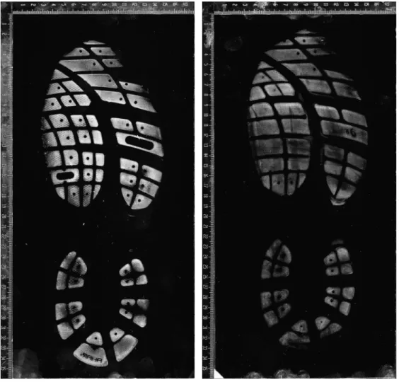
A pair ofAsics-brand men’s sneakers were worn by the forensic scientist every day over the course of a year in an urban environment. The outsoles consisted of approximately 63block features of varying size and shape. Impressions of both outsoles were captured every fortnight; yielding 52 impressions including week 0 (regrettably, impressions were not made for week 4). These impressions were captured using the gel-lift method, usingbvda-brand gel-lifters, and then scanned into high-resolution digital negatives in the^.tifffile format. Each file is a 256-level grayscale image.

Two sample images from this dataset are shown in Figure 2.1.

(23)

(a)Right outsole on week 2. (b)Right outsole on week 44.

Figure 2.1:Original images from our dataset.

2.1 Issues

While every effort was made to remain consistent during the course of recording these impressions, many forms of unwanted features were captured in addition to the shoeprint. These included air bubbles, fingerprints, dust, debris overlapping the shoeprint, ghosting of the impression, and areas of missing detail. The observations given below were made while studying the dataset:

• Debris consists of different sizes/materials—some appear to be fibres caught on outsole, and others are larger unidentified artefacts.

(24)

• Some debris appear to have been dislodged in the process of imprinting; leaving areas of the outsole missing in detail.

• All of the images have varying levels of (apparent) fingerprint noise. In the worst cases (e.g.

week 0), the fingerprint partially occludes the outsole impression.

• Certain regions of the outsole (e.g. ridges above right side of heel) appear in a few of the prints but are missing/weak in others.

• All the images have some noise in the form of debris, but they are most notable in the prints from weeks 0–30.

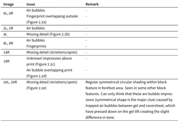
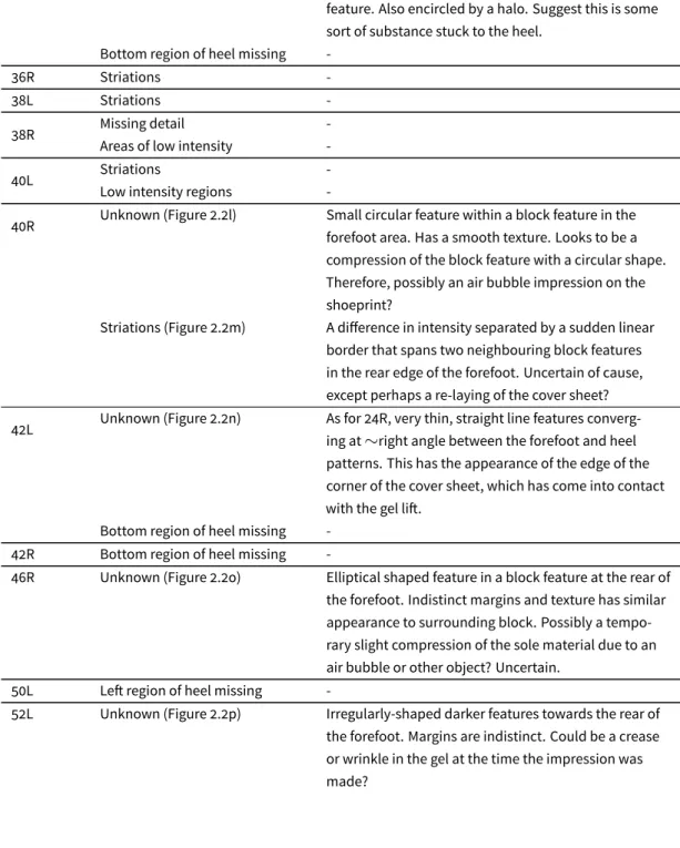
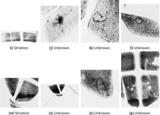
Table 2.1 provides a comprehensive list of the issues that were deemed to be potentially problematic to the performance of the model, accompanied by the comments of the forensic examiner where relevant, and figures to aid the reader’s comprehension.

Table 2.1:A list of issues found with the dataset.

Image Issue Remark

0L, 0R Air bubbles -

Fingerprint overlapping outsole (Figure 2.2a)

-

4L Missing detail (Figure 2.2b) -

Fingerprints -

14R Missing detail (striations/spots) - 18R Unknown impression above

print (Figure 2.2c)

-

Air bubble overlapping print (Figure 2.2d)

-

20L, 20R Missing detail (striations/spots) (Figure 2.2e)

Regular symmetrical circular shading within block feature in forefoot area. Seen in some other block features. Can only think that these are bubble impressions (symmetrical shape is the major clue) caused by trapped air bubbles between gel and coversheet, which have pressed down on the gel-lift creating the slight difference in tone.

(25)

Table 2.1continued

22L Ghosting (Figure 2.2f) Ghosting over block features at toe region. Yes, reposi- tioning is the reason for the doubling of the impression in this region. Despite best efforts, training and experience, it is still possible to experience slight shifting of the shoe during the printing process, especially at either end of the shoe.

Missing detail (striations) -

22R Bleeding -

Striations -

24R Unknown (Figure 2.2g) Very thin, straight line features converging at∼^right

angle between the forefoot and heel patterns. This has the appearance of the edge of the corner of the cover sheet, which has come into contact with the gel lift.

26L Unknown / Ghosting (Figure 2.2h)

Ghosting over and between block features on the toe region. Possibly light contact between the toes/front region of the sole and the gel? Not clear so I’m uncertain.

28L Missing detail -

28R Bottom region of heel missing - 30L, 30R Overlapping fingerprint - 32L Regions of low intensity through-

out print

-

32R Horizontal striation (Figure 2.2i) Two straight-edged bands running across width of forefoot, producing a darker region than surrounding block features. Uncertain about cause of feature. Possibly underlying features beneath the gel when print was made (unlikely as floor is flat linoleum)?

Low intensity regions -

34L, 34R Heel impression very weak; lots of detail missing

-

34R

Striations -

Regions of low intensity -

Missing detail -

Unknown mark (Figure 2.2j) Large, bright irregularly-shaped features within block features in heel and forefoot, with accompanying smaller features. Appears to be a reflective surface con- tamination on the shoe sole? Possibly debris of some description? Uncertain.

36L

Striations -

(26)

Table 2.1continued

Unknown mark (Figure 2.2k) Amorphous, irregularly-shaped feature in a block feature in the heel area, with a particulate texture that has a different appearance than the surrounding block feature. Also encircled by a halo. Suggest this is some sort of substance stuck to the heel.

Bottom region of heel missing -

36R Striations -

38L Striations -

38R Missing detail -

Areas of low intensity -

40L Striations -

Low intensity regions -

40R Unknown (Figure 2.2l) Small circular feature within a block feature in the forefoot area. Has a smooth texture. Looks to be a compression of the block feature with a circular shape.

Therefore, possibly an air bubble impression on the shoeprint?

Striations (Figure 2.2m) A difference in intensity separated by a sudden linear border that spans two neighbouring block features in the rear edge of the forefoot. Uncertain of cause, except perhaps a re-laying of the cover sheet?

42L Unknown (Figure 2.2n) As for 24R, very thin, straight line features converging at∼right angle between the forefoot and heel patterns. This has the appearance of the edge of the corner of the cover sheet, which has come into contact with the gel lift.

Bottom region of heel missing - 42R Bottom region of heel missing -

46R Unknown (Figure 2.2o) Elliptical shaped feature in a block feature at the rear of the forefoot. Indistinct margins and texture has similar appearance to surrounding block. Possibly a tempo- rary slight compression of the sole material due to an air bubble or other object? Uncertain.

50L Left region of heel missing -

52L Unknown (Figure 2.2p) Irregularly-shaped darker features towards the rear of the forefoot. Margins are indistinct. Could be a crease or wrinkle in the gel at the time the impression was made?

(27)

Along with possible explanations for the issues, the following general comment was provided:

Interesting to read your note regarding the amount of debris in weeks 0–30. The difference would coincide (week 32) with when I started to tape lift the shoe soles prior to printing. I finally looked at the scanned images that were being sent back to me and noticed the large amount of debris on the soles. Knowing that this would impact on the subsequent analysis of the data, I started cleaning the soles with the tape lifts.

Given this information, we speculate that the tape lift method might be responsible for the in- consistent appearances in intensity (striations and spots) observed in the latter half of the dataset.

Perhaps some residue from the tape was left behind on the outsole and then transferred to the gel while imprinting.

Out of the issues identified above, the most egregious was determined to be the debris which appeared to consist of fibres and other objects that were transferred from the outsole and onto the gel in the process of imprinting. The debris was particularly problematic due to it obscuring regions of interest in the shoeprint. For the purpose of our research we refer to these unwanted features that obscure the object of interest asnoise. To correct this noise, we returned to the literature and surveyed the denoising methods presented there.

(a)Fingerprint. (b)Missing detail. (c)Unknown. (d)Air bubble.

(e)Spot. (f)Ghosting. (g)Unknown. (h)Unknown.

(28)

(i)Striation. (j)Unknown. (k)Unknown. (l)Unknown.

(m)Striation. (n)Unknown. (o)Unknown. (p)Unknown.

Figure 2.2:Crops of the dataset revealing specific instances of the issues detailed in Table 2.1.

2.2 Prior work

In the following, we briefly survey the existing methods that address noise found on shoeprints.

It should be noted that these methods have been developed to analyse impressions or photographs of shoeprints taken from the crime scene, and then compare them against reference shoeprints in a database. The datasets used for reference shoeprints typically consist of a single instance of a given model of shoe. In such scenarios, finer details of the prints can be discarded. In contrast, our dataset consists of high-resolution impressions of one shoe taken in the laboratory every fortnight—thus capturing the development of low-level characteristics on the outsole.

In Kong et al. [52], their pre-processing steps for photographs taken from the crime scene in- clude manually rotating and cropping the shoeprint out of the photograph; then binarising the image and applying median filters and morphological operators which delivers the input to their feature extraction algorithm. Srihari and Tang [8] discuss the various approaches to enhancing image quality including thresholding and edge detection; they compare the performance of popular methods in each approach and evaluate the results. Li et al. [53] developed a preliminary pre-processing

(29)

stage as part of their shoeprint retrieval algorithm. They smooth the crime scene image with a low- pass filter, perform an adaptive binarisation, followed by morphological operators to arrive at the final image. Li and Wang [56] have used noise filtering, contrast enhancement, and edge detection as preliminary steps to their shoeprint positioning algorithm. Alizadeh and Kose [58] eliminate noise by median filtering followed by thresholding, rotation, and scaling of the shoeprint. Wang et al. [60] have detailed a manifold ranking method for shoeprint retrieval which involves thresholding, rescaling, and rotating as pre-processing steps. Zhang and Allinson [29] have smoothed noisy figures using anisotropic filters. Dardi et al. [44] have employed histogram equalisation and edge detection as part of their shoeprint retrieval pipeline. Jing et al. [40] transform colour figures into grayscale, apply block-based noise removal using a Gaussian low-pass filter, extract edges using a Sobel filter, and finally apply principal component transform to rotate the figures. Luostarinen and Lehmussola [62] conducted an independent empirical evaluation of automatic shoeprint retrieval methods and concluded that novel pre-processing methods were still desirable.

Additionally, we attempted to employ state-of-the-art image denoising filters such as bm3d [82]

and non-local means [83]. We found these methods to deliver no discernable improvement in the image quality of our wear-and-tear dataset.

The survey of the existing literature did not yield any suitable methods to fit our purposes. Apply- ing these methods to our dataset resulted in a clearer denoised image, while also destroying the low- level features of the outsole that characterise the wear-and-tear pattern. These features are essential for the task of studying and modelling the wear pattern. The existing methods have been designed as pre-processing methods that fit into larger shoeprint retrieval systems and denoise shoeprints at the cost of image clarity and definition. Our principal concern in developing a denoising method for this dataset was to efficiently mitigate noise, while maintaining high-level features of the outsole and the low-level wear patterns. The denoising method we developed to satisfy these unique constraints is described next.

2.3 Proposed denoising methodology

Starting with the digital negatives, each of the 52 figures were processed individually to be denoised. In the first step, the complement of the negative was taken. The image was then examined to determine if its intensity needed to be adjusted. Due to variations in the amount of pressure applied while capturing the impression, some of the figures are of a weaker intensity than others.

After analysis of the image and its histogram, the intensity of the image was scaled to the full 0–255 grayscale spectrum, if required. A binary mask of this image was then created using the adaptive

(30)

thresholding algorithm, using a sensitivity level parameterised byα. Due to the variation in overall intensity levels among the impressions, a slightly aggressive value ofαensured that the maximum amount of the shoeprint was captured, but this came with the cost of capturing much of the noise present in the background of the image. To deal with the additional noise in the binary mask, noisy regions were marked using region-of-interest (roi) polygons and then filtered out. This step ensured that the shoeprint mask remained intact while background noise was filtered.

(a)Complemented and cropped shoeprint.

(b)Binarised image. (c)Binary mask after processing.

(d)Fully denoised image.

Figure 2.3:Print of the right shoe on week 18 through various stages of the proposed denoising method.

Using a disk-shaped structuring element with a logical neighborhood ofβ, the mask was then dilated to fill in the block regions of the outsole. Holes inside connected components were also filled in. This dilation process was repeated 4–7 times, as deemed necessary. Understandably, this process also tends to inflate background noise. The next step was therefore to erode the mask with a square-shaped structuring element using a logical neighborhood of sizeγ. Erosion was performed 3–5 times, depending upon the image. The shape and size of structuring elements were determined via experimentation. At this stage of the process, the logical mask clearly defines the pixels of the

(31)

original image that comprises the shoeprint. Using this mask we set the background of the image to be pure white, leaving the shoeprint untouched. The outputs of these steps are given in Figure 2.3.

(a)Cropped region of heel on week 4. Noise is

evident.

(b)Noise map obtained by thresholding image

2.4a at 10.

(c)Image 2.4b dilated using a 3x3 structuring

element.

(d)Fully filtered image, showing mitigated noise.

Figure 2.4:Intermediate stages of noise filtering highlighted using left shoe on week 4.

The convex hull of each block feature was computed and converted into its own binary mask.

This allowed for each block feature to be processed in isolation. The next step was to denoise the image of the debris contaminants. After an exhaustive search of methods to identify the noise in a given region of the image, the best method was determined to be a simple thresholding to obtain a noise map defining pixels of a block feature as noise, parameterised byδ. Once the noise map was obtained, we dilated it using a disk-shaped structuring element of sizeε. This step allows us to capture the borders of noise patterns while filtering. Using the noise map as a roi mask, the block feature was then filtered using an averaging filter of sizeζ. This process is then repeated for each block feature present in the outsole, to deliver a shoeprint impression free of obstructions. Figure 2.4 illus- trates the steps involved in denoising. Each image is written back to disk as an uncompressed^.tiff file.

Table 2.2:Parameters from our method and the values optimised for our dataset.

Parameter Value

α 0.6

β 7×7

γ 3×3

δ 10

ε 3×3

ζ 50×50

(32)

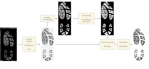
Despite the great care taken in the denoising process, the automated steps can sometimes leave noise present on the binary mask. Regions of the background may also be regarded as foreground in the thresholding process. Therefore we touch-up each image the dataset by manually examination, removing any noise that remained after filtering. Our semi-automated method was efficient enough that manual touch-ups were only required for less than 5% of the dataset. Finally, the dataset was padded to a uniform 13750×5500 size and registration was performed to align all of the prints. A block diagram outlining these steps is shown in Figure 2.5. The parameters we discovered to best fit this methodology with our dataset are given in Table 2.2.

Figure 2.5:A block diagram outlining the processing steps in the proposed method.

2.4 Evaluations

A subjective assessment of the post-processed dataset determined it to be sufficiently adequate for our purposes. The proposed denoising method identified the noisy pixels and altered it to be near inconspicuous—leaving the outsole regions that show wear-and-tear untouched.

To perform an objective evaluation, we compared our method against the baselines of median filtering and adaptive Wiener filtering, using the metric ofStructural Similarity Index(ssim) [84], defined in (2.1).

SSIM(f,g) =l(f,g)c(f,g)s(f,g), (2.1)

(33)

where











l(f,g) = _μ^2μ2^f^μ^g^+C¹ f+μ²_g+C1, c(f,g) = _σ^2σ2^f^σ^g⁺^C²

f+σ²_g+C2, s(f,g) = _σ^σ^fg^+C³

fσg+C3,

whereinl,c, andsdenote the luminance, contrast, and structure comparison functions respectively. The termfdenotes the noisy image andgthe denoised image.μandσdenote mean and standard deviation of image luminance and contrast, respectively.σfgis the covariance betweenfandg.

C₁,C₂, andC₃are positive constants employed to avoid a null denominator.

The ssim index is a positive value∈ [0,1]where 0 denotes no correlation and 1 denotesf = g.

From the results obtained after processing all figures in our dataset, we ascertain that our denoising method can improve on the ssim score of median filtering by up to 0.0465. The results are given in Table 2.3.

Table 2.3:Mean and standard deviation of SSIM scores computed over all 52 images.

Proposed Method Median Filtering Wiener Filtering

Mean 0.9143 0.8678 0.8868

STD 0.0281 0.0219 0.0250

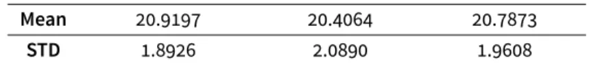
PSNR(f,g) =10 log₁₀(255²/MSE(f,g)) (2.2) Additionally, we comparedPeak Signal-to-Noise Ratio(psnr, defined in (2.2)) scores against the same baselines. Once again,fandgdenote the noisy and denoised figures, respectively, and mse is the mean squared error—i.e. mse betweenfandg. Results are given in Table 2.4.

Table 2.4:Mean and standard deviation of PSNR scores computed over all 52 images.

Proposed Method Median Filtering Wiener Filtering

Mean 20.9197 20.4064 20.7873

STD 1.8926 2.0890 1.9608

psnr scores obtained using our method see an average improvement of 0.1324 over the baseline methods. Furthermore, a subjective examination of the processed figures using the proposed method compared against the baseline filters shows that our method is much more efficient at maintaining the finer details we desire.

(34)

∗ ∗ ∗

Having surveyed the related literature and found little suited to the task of denoising a footwear impression while maintaining low-level characteristics, we designed a denoising method to fit the unique requirements of our dataset of shoeprints. This dataset captures the evolution of wear characteristics and can be used for their study. In the next chapter, we discuss the method we use to model wear, our cnn architecture, and the results of our experiments.

(35)

All models are wrong, but some are useful.

George Box

Modelling Wear Patterns 3

How does the outsole of a pair of shoes change over time? The forensic examiner’s interpretation of the shoeprint and its admissability as evidence is built through their years of experience in studying shoeprints and the individualising characteristics that contribute to the wear pattern. Such knowledge is notoriously hard to quantify. Deep learning models have made large strides in developing computational representations of domains with these traits—including in the field of forensics—

where they have been successfully applied to diverse problems like the recognition of finger vein patterns [85], orientation in iris images [86], and touchless palmprint recognition [87].

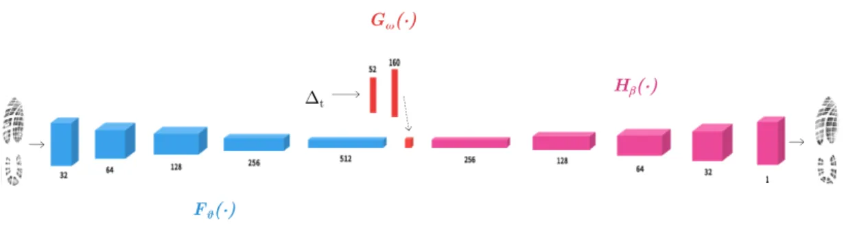
In this chapter we present a cnn architecture that performs a pixel-wise prediction of footwear outsole appearance. Our core contributions presented here are as follows—(i) we apply a cnn model to learn and predict the wear formation on our dataset of shoeprints, and (ii) an alternate model that is able to reconstruct the outsole back to its original state on a given week within a timeframe of one year.

In the following sections we first survey the related literature in the domains of deep learning and forensics & shoeprints. We proceed to detail our methodology for modelling, describe the experiments done with our models, and finally, we analyse the results of our experiments.

(36)

3.1 Related work

Using our dataset of 52 shoeprints, described in Chapter 2, we wish to learn a model of the wear pattern captured within. Once trained, this model should be capable of extrapolating the wear pattern when given a new shoeprint as input. Fundamentally, we approach this as an image-to-image regression task.

The literature contains many successful applications of deep learning to these types of dense prediction tasks; such as image in-painting [88,89], super-resolution [90], denoising [91], and image recovery from compressed representations [92]. Deep neural networks and their convolutional variants have established state-of-the-art performance over nearly all facets of computer vision tasks.

One of the primary advantages of using dnns is their ability to learn end-to-end mappings without the use of image priors, or the explicit engineering of features.

Our dataset shows the life and wear of a pair of shoes through impressions captured at evenly spaced intervals of time. To the best of our knowledge, this is the first time such a dataset has been used in the literature of deep learning. A closely related problem is video frame generation/prediction [93] that involves operations on inputs in the spatial domain, while simultaneously capturing correlations in the temporal domain. Notably, in video frame prediction, one has access to an extensive amount of data by using each frame in the video sequence as a datapoint. Finn et al. [94]

use a combination of convolutional and lstm layers to model pixel motion and optical flow. They introduce a dataset with 1.5 million video frames and a model that predicts video sequences up to 1 second in the future. Our dataset is significantly smaller in size.

3.2 Proposed modelling methodology 3.2.1 Convolutional neural networks

In this section we provide a brief mathematical background to the operation of the convolutional neural network which forms the basis of our modelling method. We start by describing a feedforward neural network (more details can be found in Goodfellow et al. [95], Chapters 6 and 9).

A learning algorithm in machine learning is essentially a mathematical function that learns a mapping between inputsx, and outputsy. Neurons are a machine learning paradigm loosely modelled after the operation of a biological brain. The artificial neuron takes the mathematical form shown in (3.1).

y=f(X

i

w_ix_i+b), (3.1)

(37)

whereinxirepresents a set of inputs that are parameterised by a set of weightswi, and added to a bias offsetb.

This linear combination is fed into what is typically a non-linearactivation function,f(z)—where z =P

iw_ix_i+b. Depending on the task or architecture,f(z)is most commonly either the rectified linear unit (relu,f(z) =max(0,z)), or the sigmoidal function (f(z) =1/1+exp(−z)). The task in ml is to learn the right values for the weightswiand biasesbithat fully approximate a set ofyvalues when given a set of knownx_ivalues.

Stacking neurons into a sequential architecture forms an artificial neural network (ann), which is capable of modelling deeper representations in more complex problem domains. anns consist of sequential layers of neurons where each neuron is independent of each other, with its own set of weights and biases. A neural network is then trained by feeding inputsxinto one end, obtain- ing predictionsyfrom the other end, computing the error of the predictions against the known values (a.k.a.ground-truth) by a pre-defined loss function, and finally propagating the error signal backwards through the network using the backpropagation algorithm [96]. The training process involves finding the optimal set of weights for each neuron so that the network best approximates the ground-truth, and is performed automatically through a convex optimiser like gradient descent.

Computer vision tasks involve inputs that are typically images—matrices that define pixel intensities, and the target outputs are either a class label for tasks such as object detection and image classification; or another image in the case of problems like denoising, in-painting, etc. In the latter, both inputs and outputs are two-dimensional matrices, therefore we define the neuron in theith row andjth column of a layer as:

y_ij =f(X

k

X

l

w_ij,klx_kl+b_ij), (3.2)

wherex_klrepresents pixel intensities of the input image in the nn’s first layer. anns have no lim- itations onwij,kl, allowing weights of a neuron to vary independently of other neurons. For images, this implies the loss of spatial context from one layer to the next.

Convolutional neural networks vary from anns in that neurons are connected locally to the output volume of the previous layer [97], performing discrete convolutions in each layer between the input volume and afilteror kernel matrix, parameterised by the weights. Convolutional layers embed spatial context of images directly into the architecture of the network. Additionally, sharing the filter weights between neurons requires only a small number of them to be stored in memory, greatly simplifying the training process. This weight sharing also exploits the property that weights useful to one section of an image might also be useful to another. Traditional cnn architectures