The views expressed are the opinions of the authors and the School of Accountancy does not necessarily agree with them. In addition, a continuous description raises questions that cannot be asked in a time series description, such as the characteristics of the transaction storm (for example, the frequency and size of transactions may vary by season and business cycle).
Identifiability
The mean is not usually µ, and may not exist
Relevant variables must be omitted
Heteroscedasticity
The model allows Sales to be negative
However, Ronen and Yaari casually mention that the variables were deflated by total power, apparently without realizing that this completely changes the analysis.
The persistence of deflated sales
Both formulas show that the persistence is α1/α2 multiplied by some random bias factor whose median is 1, but whose expected value (mean) is not 1. No doubt Dechow and Schrand (2004) would say that they were actually measuring the persistenceα3 of the asset-to-turnover ratio, assuming the process.
Adding an omitted variable
Transforming the variables
Ratios
Equilibrium growth rates
The solution of this set of equations for the vector ˆy involves the value of λ; must have y1 = 0 (which is a check on the numerical accuracy of the solution), and all other values of y are expressed as the difference from y1. Of course, this does not affect the matrix Z, which gives the logarithm of all ratios; it is defined by the differences of the y values and is not affected by adding any constant to all.
Persistence
Not only does this "cross-inertia" tend to be greater in faster-growing firms, but it tends to be greater when the ratio of variables is greater. If θ and ϕ and γS3−γA3 are all close to zero, the regression slope will be approximately constant eβS−βA and under these strong conditions this can be expected to be the persistence of the relationship.3.
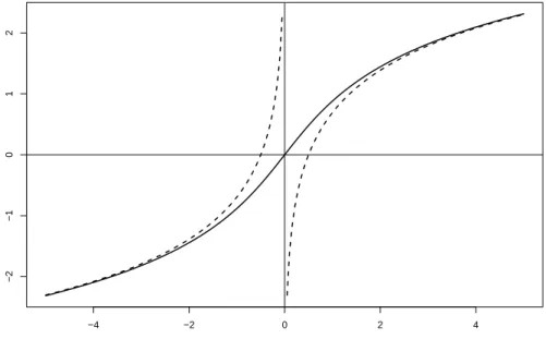
Can the log transform be generalised?
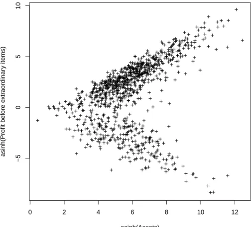
An obvious generalization of the logarithm is the inverse hyperbolic sine function yi = sinh−1(xi/θ) = log. 28) Equations (27) and (28) are written with the same scale factor θ for each variable, but this is not significant: it would be possible for each variable to have its own scale factor. Thus, the sinh−1 function behaves like the logarithm when the argument has large magnitude, and smoothly connects these two logarithmic functions with a nearly straight line through the origin, as shown in Figure 1. Consider the behavior of profit as a function of assets (the data is a random sample of 1,000 firm-years of global manufacturing firms), shown in Figure 2.
The source of the problem is that a firm with $100 million in assets will have profits or losses of several million dollars (say, most likely between -5 million and +5 million). There is a fairly high probability that the winnings will be between $1 million and $5 million, a smaller but still moderate probability that they will be between -$1 million and -$5 million, but almost no probability that they be between $1,000 and $5,000. The density is bimodal, with the peaks moving further as the scale increases, and this is just the first pattern in Figure 2.
Negative values are differences of other values
Although the sinh−1 looks attractive at first glance, it cannot work with an equation such as equation (17). debit balance instead of the usual credit balance). However, if we can operationalize the underlying non-negative variables, then we can estimate their evolution over time using equation (17), and subsequently extract the required differences from the forecast values. In this way, we can construct non-negative accounting values that have meaning and from which the desired values can be retrieved.
We can fit parameters β and Γ in equation (17) using the logarithms of these non-negative variables (for example in a single industry), and estimate the covariances of the residuals. If we know the values of y up to time t−1, we can estimate the vector yt and its covariances, which are assumed to be multivariate normal. If desired, simulation can be applied to equation (17) with the fitted parameters, to show the evolution of the financial statements of a typical firm in the fitted industry.
Predictions
In principle, one could use these ideas to develop formulas for the persistence of relationships such as return on assets, where the numerator does not have to be positive and must therefore be expressed as a difference between two positive variables, or even return on equity, where both numerator and denominator must be expressed as such. These predictions typically concern the magnitude of some number, not just the sign of a ratio. For example, if actual fixed growth rates are around 10% and the theory predicts they should be around 25%, the theory clearly fails even though the prediction has the correct (positive) sign.
But if theory predicts that growth rates should be around 11%, this can be taken as strong support that it reflects an important feature of economic reality, even if a large-sample hypothesis test could show that 10%. If these predictions seem substantially consistent with the empirical evidence, then the resulting model should be significantly more robust than previously used models, such as those of Ronen and Yaari (9.1).
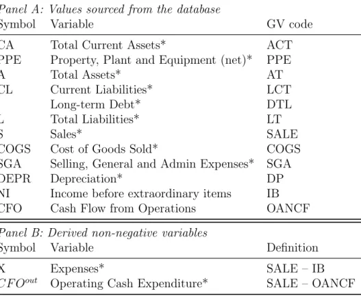
Data
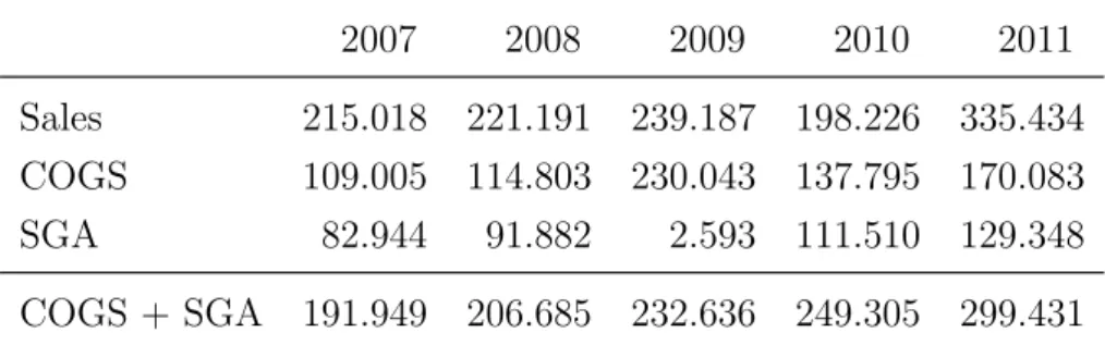
The result is that any model that reasonably predicts SG&A to be around 100 in 2009 will be wrong by a factor of 40, about 9 standard deviations. I examined some cases where the residuals from the model were extreme outliers (at least eight times the standard deviation and therefore with a probability of less than 1 in 1015). There are two kinds of explanations for such outliers: one is that the model is wrong, so that the distribution of errors is not as expected; the other is that the specific data points are in error.
After investigating several cases similar to Forbes Co Ltd, it appeared that mergers or splits or defective data were the usual explanations, so the correct treatment is to delete these points from analysis. Accordingly, I present results using all data points and again after removing firm-years where one or more residuals exceeded 4 standard deviations (about 1 chance in 16,000).
Results
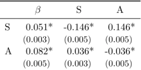
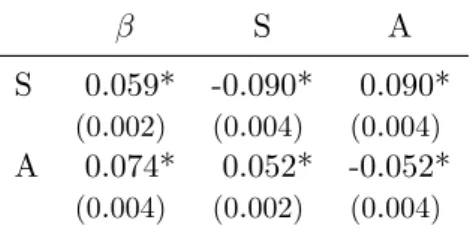
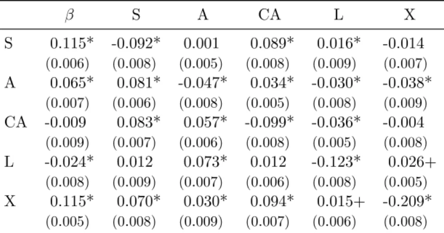
However, Table 3 shows that the picture changes if the estimation efficiency is improved by imposing the constraint that the sum of each row of Γ must be zero. The efficiency gain from the imposition of a constraint appears to be significant, although violations of the constraint are not serious if it is not imposed. However, the moments and correlations of the residuals are not significantly affected by the change in score.
This reduces the moments of the residuals (as it should), but it does not bring much improvement in the closeness of the other statistics to the theoretical expectations. As more variables are added to the accounting vector, the standard deviations of the residuals decrease, but only slightly; higher moments and correlations do not change much. Second, equation (17) can be taken as a definition of the disturbances, and the residuals can be regressed on the hypothesized causal variables.
The Jones model for earnings management
But there is also a serious omitted-variables problem, since α must scale with firm size. It is therefore difficult to justify the interpretation that the remaining part of the event period represents earnings management rather than simply a misspecification of the model. Accrualst=CF Ooutt −Xt (30) with a confidence interval which can be found from the covariances of the residuals εCF Oout and εX.
The lognormal distribution is well known (eg Aitchison and Brown, 1966), but little is known about the distribution of sums of lognormal values and almost nothing about the distribution of the difference. The only paper that appears to examine the distribution of the difference is Lo (2012); Lo cites several earlier papers, but all seem to consider only approximations of the sum. The distribution of the sums and differences must be significantly different because the sum can only have positive values.) Lo gives a closed-form approximation (its equation 2.11) which is a shifted lognormal, along with a series expansion to correct the approximation (2.16) . In practice, the required confidence intervals can be estimated by simulation, since the parameters of the basic model (including the correlations between the logarithms of the non-negative variables) are known.
Residual income valuation of firms
It can be estimated from all firms in the same industry, as the parameters Γ and β are driven by underlying economic, technical and managerial factors that are likely to be the same across an industry. This identity applies regardless of the accounting principles used, as long as they comply with the requirement of net profit. Since the future values of income and equity are unknown, they must be estimated on the basis of the latest available accounts.
Given the current financial vector x0, where x contains at least the variables R, X, A and L, we can repeat equation (17) to find the expected value of x (and hence N I =R−X and Q=A−L) for each year in the future, and the sum in equation (31) can be explicitly calculated. There is no need to use a fixed forecast period, since the result of the iterative equation (17) automatically converges to the appropriate growth rate for a company in this industry. Of course, if better company-specific information is available, it can be used to refine this naïve estimate, but the model already provides strong guidance on which future income and equity trajectories are likely.
Financial distress
168 Dividend imputation in the Context of Globalisation: Extension of the New Zealand Foreign Investor Tax Credit Regime to Non-rezident Direct Investors, by B. 166 An Exploratory Investigation into the Delivery of Services by a Provincial Office of the New Zealand Inland Revenue Department, avtor S. 165 The Practical Roles of Accounting in the New Zealand Hospital System Reforms An Interpretive Theory, avtor K.
141 Accounting Information Systems Course Curriculum: An Empirical Study of the Views of New Zealand Academics and Practitioners, by G. 140 Balance Sheet Structure and the Managerial Discretion Hypothesis: An Exploratory Empirical Study of New Zealand Life Insurance Companies New, by An Analysis3911. i The contemporary movement between cash flow and accrual-based performance numbers: Evidence from New Zealand by J.
126 The Finance Function in Healthcare Organisations: A Preliminary Survey of New Zealand Area Health Boards, af K. 90 Chartered Accountants in the New Zealand Public Sector: Population, Education and Training, and Related Matters, af K.