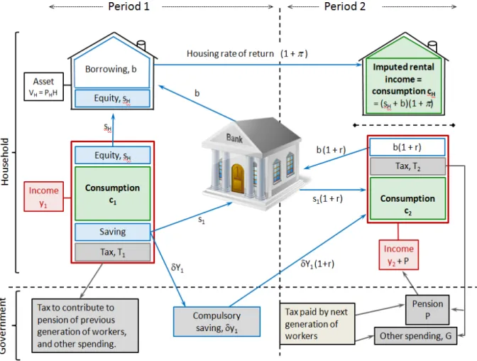
The approach adopted here is based on a two-period model and focuses on the life plans of a representative household.2 The household works and earns income, y1, during the period. While a larger number of periods could be included to capture more detail about household life-cycle events and housing decisions, this level of detail would unnecessarily complicate the analysis without yielding additional insights.3 The household is assumed to maximize utility from consumption composite consumption good in each period, denoted by c1 and c2.
Mortgage Borrowing
A Compulsory SAYG Scheme
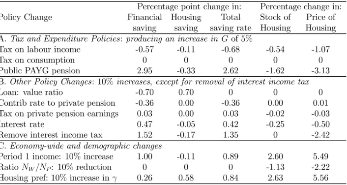
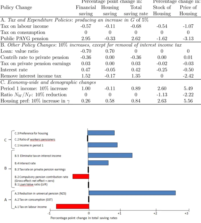
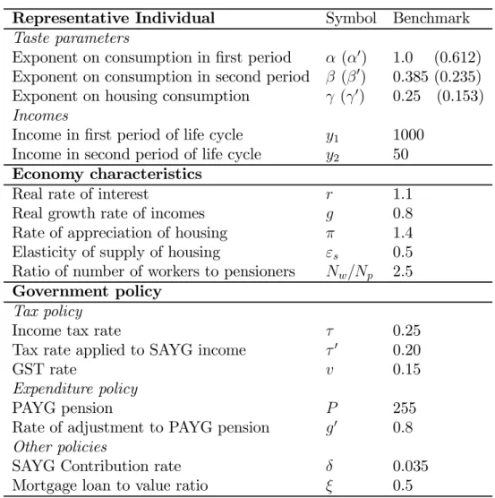
The standard PAYG pension is set at 255, just under a quarter of working-age earnings. The second category consists of 'other policy changes', such as changes in the loan-to-value ratio, ξ, the mandatory SAYG pension contribution rate, δ, and the interest rate, r.
Changes for which G is Constant
These are changes over which the government would not be expected to control, and include changes in the demographic ratio, Nw/Np, the level of income in the first period of life, y1, and the preference for housing, γ. As with the second category, changes in these variables have different consequences for G, but this is just another endogenous variable of interest for comparing changes: there is no reason to force common changes in G for all simulations in this group. Similarly, the effect on savings of a change in inv that produces the same effect on G is given simply by replacing τ in (26) with v.
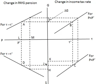
The left-hand side of the diagram illustrates the effects on total saving, S, and spending, G, of changes in the exogenous PAYG pension, P, for a given tax rate, τ =τ∗. The right side of the diagram shows variations in S and G for variations in the tax rate, τ, for a given pension, P =P∗. Therefore, from the right-hand side of the diagram, an increase in iτ, which produces a change of ∆G in public expenditure, with P held constant at P∗, is associated with a reduction in savings measured at length JK.
To achieve an equivalent increase in non-transfer expenditure with a policy of reducing P, holding the tax rate constant at τ∗, one would have to reduce P by LM, resulting in an increase in total savings JH.
Changes in The Price of Housing
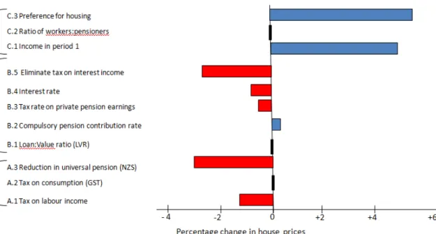
When examining the comparative statics of the model, the assumption regarding the price elasticity of housing supply is εs = dpdH/H. First, omitting the time subscript and differentiating (27) yields the following: 30) Thus, the proportional response of house prices in period 1 to a change in housing expenditure, VH, is positive unless supply is infinitely elastic, and is inversely proportional to the elasticity of the housing supply. This section reports the comparative statistical results for a number of policy changes in the tax and expenditure structure.
These include changes to the rate of income tax, the rate of consumption tax and the level of the PAYG public pension. To make these three tax and expenditure policies comparable, their effects are simulated on the basis of a change which, in each case, results in the same change in non-pension public expenditure, as explained in the previous section. In this way, the government's budget constraint is met and the effect of each of the policy options on any of the endogenous variables is directly comparable.
Suppose it is desired to increase G by 5%: what are the implications of financing this extra non-transfer expenditure by increasing τ or v, or decreasing P.
A Change in the Income Tax Rate
A Change in the Consumption Tax Rate
A Reduction in the PAYG Public Pension
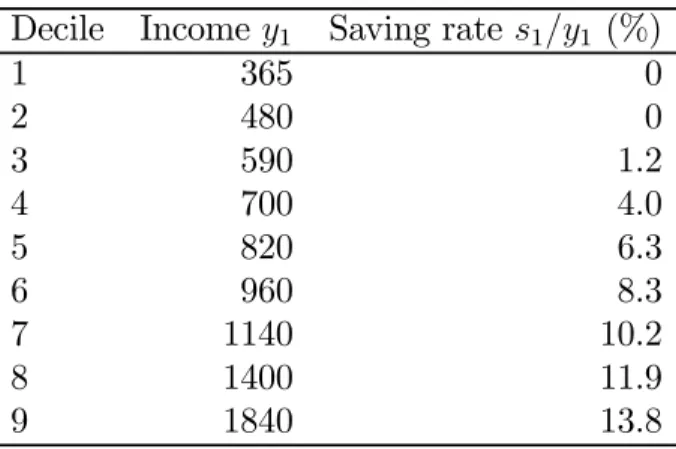
This is in accordance with the current study, which finds, as a result, that a decrease in the universal pension is accompanied by an increase in financial savings. 19. To further explore the implication of the PAYG pension, it is possible to consider the optimal plans for alternative levels of individual income values in the first period, y1, given the standard arithmetic mean value of y¯1 = 1000. Suppose that this mean is related to a lognormal distribution with a logarithm variance of 0.4.20 The results are summarized in Table 2 for the deciles of the distribution.
However, the table shows a zero savings rate at the lowest two decile values of y1: this is due to the limitation that the only form of borrowing is through the mortgage. The finding that incomes in the lowest deciles have no incentive to save in view of government pensions is consistent with the findings of Scobie, Gibson and Le (2004) for New Zealand, and Moore and Mitchell (1997) and Bernheim (1992) for the United States. Similar results are reported for Great Britain by Attanasio and Rohwedder (2003), and for Italy by Attanasio and Brugiavini (2003).
The results are based on a 10% change in the policy variable, and unlike the tax and expenditure changes, the level of public, non-pension expenditure, is not held at a constant level across all policy simulations.
A Change in the Loan-to-Value Ratio
A Change in the Compulsory Saving Rate
The model can be used to investigate whether the existence of a compulsory contribution will result in an increase in the overall level of saving, or simply lead to a corresponding reduction in private financial saving. Households were found to fully offset the effect of a compulsory savings scheme by a proportional reduction in voluntary private savings.22. Instead of simply considering the introduction of a SAYG scheme in this way, suppose a scheme is introduced with a compulsory rate of 6%, but the universal pension is reduced in a way that the total retirement income of PAYG and SAYG schemes preserved (that is, income from private financial savings excluded), while the tax rate is unchanged.
Alternatively, assume that the SAYG scheme is introduced at a mandatory rate of 6% and P is reduced so that G can increase by 5%. In this case, the economic saving falls by 24% and P must be reduced by a third. Finally, suppose that the SAYG scheme is introduced, again with a mandatory rate of 6%, and that total pension income remains unchanged at the original level, while G is increased by 5%.
A Change in the Tax Rate on Interest in the Compulsory Pension
A Change in the Interest Rate
Housing savings increase by 8.2%, partly to offset higher mortgage repayment costs, but at the same time overall housing demand falls by 0.75%. Interest income from mandatory savings also increases, bringing an increase in the private pension by 4.7%. The higher interest rate means higher tax revenue, which, through the government budget constraint, means a small increase in G of 0.86%.
Eliminating Taxation of Interest Income
This is accompanied by an increase in the private pension as the accumulations of the compulsory saving element are strengthened by the now tax-free income for all savings. There is also an increase in financial savings (17%), partially reflecting a shift from housing savings.24 The rate of financial savings increases by 1.5 percentage points, while housing savings decreases by 0.2 percentage points. The net result is an increase in the overall household saving rate of 1.4 percentage points, measured as a percentage of gross income.
For example, if the tax rate were to be lowered from 0.25 to 0.20 instead of eliminated, the savings rate would increase by approximately 0.28 percentage points. The increased savings rate after the abolition of the tax on interest income refers to economic savings during working life (period 1 in the model). In this case, the tax rate on earned income must increase from 0.25 to 0.27, while the total savings rate increases by 1.3 percentage points.
If G is held constant at its base level when the tax on interest income is removed, then the labor tax rate must rise from 0.25 to 0.255, and the overall saving rate rises by 1.8 percentage points.
A Rise in Income
Population Ageing
The benchmark case assumes that P grows at the same rate as labor income (that is, g =g) and thus maintains a constant relationship with average wage growth. The growth rate of P, set at 2% per year in the benchmark case, had to be reduced by one percentage point. In other words, the PAYG pension would grow in real terms at half the growth rate of the average wage.
Therefore, consumption falls slightly in both periods, financial and total savings rise slightly, and housing savings fall slightly. 27. An alternative policy response to population aging is to maintain a constant total pension income from PAYG and mandatory SAYG schemes combined, along with G, without raising taxes. The problem is then to find a mandatory savings rate and a corresponding reduction in P, so that the total pension income from P combined with the private pension remains constant, as does the level of public expenditure per inhabitant, G.
The solution, which can be found through a process of trial and error, is to increase the mandatory contribution, δ, from 3.5% to 6.5% of gross income in period 1 and to increase P by 22% reduce.
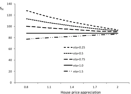
Changes in the Preference for Housing
An increase in the tax rate on labor and interest income reduces savings rates and lowers demand in the housing market. The loss of tax revenue is compensated by a reduction of approx. 1.7% in public non-pension expenditure, while the real value of the universal pension is kept unchanged. Particular attention in the simulations was given to the potential impact on household savings rates of a number of policy changes.
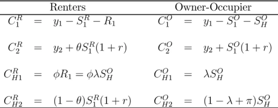
The two-period model of this article assumes that the representative individual does not buy a house in the second (retirement) period of the life cycle. The fundamental choice considered here is to be a tenant (type-R) in period 1 and to buy a property to live in in period 2; or to be the owner in period 1 (type-O) and to live in the house in both periods. Housing consumption in the later period also benefits from the appreciation of the asset at rate π.
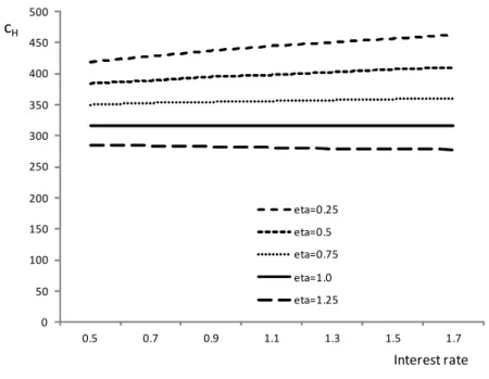
Consider the elasticity of c1 with respect to a change in the interest rate. the elasticity of c2 with respect to is:. Above, it was found that changes in the interest rate had a negligible effect on housing consumption. Consequently, the result in the paper does not derive from the choice of η, but from the operation of the government budget constraint.