The recruitment dynamics of post-settlement juvenile toheroa and the potential applications for aquaculture

(1)

http://researchcommons.waikato.ac.nz/

Research Commons at the University of Waikato

Copyright Statement:

The digital copy of this thesis is protected by the Copyright Act 1994 (New Zealand).

The thesis may be consulted by you, provided you comply with the provisions of the Act and the following conditions of use:

 Any use you make of these documents or images must be for research or private study purposes only, and you may not make them available to any other person.

 Authors control the copyright of their thesis. You will recognise the author’s right to be identified as the author of the thesis, and due acknowledgement will be made to the author where appropriate.

 You will obtain the author’s permission before publishing any material from the thesis.

(2)

i

The recruitment dynamics of post-settlement juvenile toheroa and the potential applications for aquaculture.

A thesis

submitted in partial fulfilment of the requirements for the degree

of

Master of Science (Research) in Ecology and Biodiversity at

The University of Waikato by

Marieka van der Lee

2022

(3)

i

Abstract

Managing the recovery of threatened species due to anthropogenic disturbance is one of the most challenging problems in ecological monitoring. Researching species ecology is vital to help us improve ecosystem health and subsequently develop better management strategies in the environment. Humanity is entirely reliant on ecosystem services for food security. With the world population expected to reach ten billion by 2050, there is a growing need for more sustainable food sources. With the exploitation of many environmental resources worldwide, aquaculture has been championed as a sustainable option for future seafood production. In New Zealand, the toheroa (Paphies ventricosa) has been identified as a potentially valuable asset to the aquaculture industry and for possible conservation strategies via the implementation of reseeding populations with hatchery-reared spat.

Toheroa faced inadequate resource management and exploitation in the 1900s which ultimately led to the closure of an important recreational, cultural and commercial fishery. However, toheroa populations have failed to recover despite over 40 years of protection. It has been proposed that the continued decline of toheroa populations is not due to a lack of juvenile recruitment. Very little is known about juvenile toheroa recruitment, and there is no available information that could facilitate restoration management or determine the appropriate action to take for monitoring juvenile populations. From both a conservation and an aquaculture perspective, understanding the underlying ecology will be pivotal for future endeavours.

My thesis aimed to investigate the distribution dynamics of post-settlement juvenile toheroa on Ripiro Beach and the potential applications for aquaculture. Population surveys were conducted on Ripiro Beach in February and May to establish a sampling methodology that accurately captures the juvenile population both spatially and temporally. Surveys on vertical substrate stratification significantly affected both density and shell size with increasing sediment depth. Additionally, in contrast to the hypothesis formed on the basis of traditional knowledge that

(4)

ii

juvenile distribution is limited to the dunes and upper intertidal, spat appeared to have far more varied littoral distributions than previously theorised. The data from these surveys were used to make estimates of the total juvenile population on Ripiro Beach with attention to changes spatially (habitat type), temporally (seasonally), and by size cohorts (mm). My results indicated that toheroa populations are not recruit-limited. Estimates for the total February population ranged between 580 (±190) million and 650 (±200) million. By May, large abundance losses (> 90%) dropped the estimated population to between 30 (±15) million and 37 (±17) million, indicating significant bottleneck mortality during the early growth stages. However, the high abundances of small spat (< 5 mm) indicate that toheroa aquaculture is potentially viable. In aid of future aquaculture applications, I investigated how handling, harvesting, and different transportation methods could impact toheroa health, survival, or performance. This experiment aimed to mimic real-world applications wherein juvenile spat would be harvested and ongrown in hatcheries.

To do this, I utilised the burrowing behaviour of juvenile toheroa as a quantitative indicator of stress. I found that if appropriate storage methods were implemented, initial handling and harvesting had a greater impact than actual transportation.

The research in this thesis demonstrated that populations do not appear to be recruit- limited. Furthermore, the findings indicate that aquaculture built on the foundation of wild-harvested juveniles is potentially viable. However, further research is required in order to quantify potential annual recruitment variation both spatially and temporally. Additionally, in order to establish a conservation approach, we must first define the niche requirements of toheroa to determine the obstacle (or obstacles) inhibiting recovery.

(5)

iii

Acknowledgements

To begin with, I would like to express gratitude for the experience of gaining such an educational experience. There are many people I would like to thank for their guidance and help that made this thesis possible. Firstly, to my supervisors Dr Phil Ross, Dr Hazel Needham. Hazel, thank you for your input, encouragement, and positivity. Phil, thank you for the amazing opportunity to be a part of something as special as the iconic toheroa, their charisma made the long drive up north well worth it. Thank you for your wisdom and guidance during this process, it couldn’t have been done without you.

Thank you to all of Team Toheroa. I would like to thank those who spent hours on the beach with me helping to collect my data during surveying, one of the many parts of being an ecologist requires being hunched over a sieve. Thank you, Ethan and Martyn for being of great assistance and putting in the hours on the beach with me.

To my family, Mum and Dad, thank you for all the love and support you’ve given me over the years. To my brothers, Jacob and Luke, thank you for always making me laugh when I need it. I would like to thank my lovely Oma, morning coffees with you always leave me feeling brighter. To my friends, Helena, Brittnee, Charlotte, Nicole, Caleb, Kelsey, and Dylan, thank you for rallying me through this thesis.

This research could not have been completed without the aid of a University of Waikato Research & Enterprise Study Award.

(6)

iv

List of Figures

Figure 1: The distribution of toheroa in New Zealand, major populations are underlined. Figure reproduced from: Ross et al. (2018a). ... 4 Figure 2: Left – Juvenile toheroa and tuatua that show shell morphological differences. Right – Adult toheroa with foot (or tongue) extended.

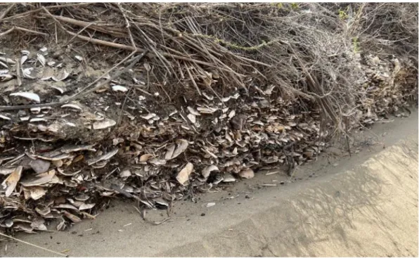
Animals found on Ripiro Beach in February 2022. ... 5 Figure 3: The internal anatomy of toheroa (Paphies ventricosa), with the left valve and mantle removed. Figure reproduced from Rapson (1952). ... 6 Figure 4: Archaeological shell middens found on Ripiro Beach in February 2022.

... 7 Figure 5: Sandstone cliffs and stream outlet on Ripiro Beach in February 2022.

(Drone photo by E. Russell). ... 16 Figure 6: Map displaying the section of Ripiro Beach where pilot surveys were conducted. Image retrieved from Google Earth ... 17 Figure 7: Fieldwork conducted on Ripiro Beach in February. ... 18 Figure 8: Photos taken of toheroa collected on Ripiro Beach that were later analysed in Fiji ImageJ. ... 19 Figure 9: Left - Mean density of toheroa per 0.25 m² quadrats at three different depths. Right - Mean toheroa shell size per 0.25 m² quadrats at three different depths. Error bars represent standard deviation (n=321). .... 21 Figure 10: Example quadrat from the three different sediment depth stratifications on Baylys Beach. ... 23 Figure 11: Line graph representing significant difference (p < 0.01) in the density of toheroa per 0.25 m² at different sediment depths along the transect.

The density of toheroa is higher in the top 0-2 cm (n=1,326). ... 24 Figure 12: Box plot representing significant (p < 0.05) difference in the median shell length of toheroa per quadrat (0.25 m²) at different sediment depths (n=1,326). ... 25 Figure 13: Schematic plots showing previously theorised distribution patterns compared to observations made on Ripiro Beach in 2022. ... 27 Figure 14: Example of twin siphon holes found on Ripiro Beach. ... 31 Figure 15: Map displaying the section of Ripiro Beach where the survey was conducted. Red dots represent sampling locations, arrow shows the length of the beach the sampling covered (14.7 km). Coordinate system:

WGS 1984 Web Mercator (auxiliary sphere). Spatial data obtained from ArcGIS pro: World Topographic Map. ... 32 Figure 16: Topography of the different sites sampled in this study. Image retrieved from Google Earth. ... 34 Figure 17: Drone photos from fieldwork in February on Ripiro Beach. (Photo from E. Russell). ... 36

(10)

viii

Figure 18: Heat map displaying density distributions on Baylys Beach in February.

Numbered labels with circle icons represent plots, with 1 on the low tide zone moving toward the high tide zone. Coordinate System: WGS 1984 ... 39 Figure 19: Heat map displaying density distributions on Maramoenui in February.

Numbered labels with circle icon represent plots, with 1 on the low tide zone moving toward the high tide zone. Coordinate System: WGS 1984. ... 40 Figure 20: Heat map displaying density distributions on Maramoenui in May.

Numbered labels with circle icon represent plots, with 1 on the low tide zone moving toward the high tide zone. Coordinate System: WGS 1984. ... 40 Figure 21: Heat map displaying density distributions on the non-bed site in February. Numbered labels with circle icon represent plots, with 1 on the low tide zone moving toward the high tide zone. Coordinate System:

WGS 1984. ... 41 Figure 22: Heat map displaying density distributions on the non-bed site in May.

Numbered labels with circle icon represent plots, with 1 on the low tide zone moving toward the high tide zone. Coordinate System: WGS 1984. ... 42 Figure 23: Heat map displaying density distributions on Mahuta Gap in May.

Numbered labels with circle icon represent plots, with 1 on the low tide zone moving toward the high tide zone. Coordinate System: WGS 1984. ... 43 Figure 24: Heat map displaying density distributions on the Island site in May.

Numbered labels with circle icon represent plots, with 1 on the low tide zone moving toward the high tide zone. Coordinate System: WGS 1984. ... 43 Figure 25: Shell size frequency distributions at Baylys beach in February for 0-5 cm sediment depth. 0 m = low tide. ... 45 Figure 26: Shell size frequency distributions at Maramoenui, sediment depth 0-5 cm. 0 m = low tide. ... 46 Figure 27: Shell size frequency distributions at Mahuta gap and The Island in May, sediment depth 0-5 cm. 0 m = low tide. ... 48 Figure 28: Shell size frequency distributions for the transect on the non-bed habitat,

sediment depth 0-5 cm. 0 m= low tide. ... 49 Figure 29: Mean shell size (mm) frequency distributions on the adult bed excavation in May. Two depth stratifications of 0-5 cm, and 5-10 cm sediment depth. Error bars represent standard deviation. ... 50 Figure 30: Adult toheroa sampled in May on Ripiro Beach. ... 51 Figure 31: Schematic plots showing previously theorised distribution patterns compared to observations made on Ripiro beach in 2022. ... 55

(11)

ix

Figure 32: Map of the study location. Red dots represent the 29 streams, and yellow outline represents the beach area that was disregarded for estimation due to different environmental conditions. Map generated in Google Earth and ArcGIS pro, Coordinate system: WGS 1984 Web Mercator (auxiliary sphere). Spatial data obtained from ArcGIS pro: World Topographic Map. ... 63 Figure 33: Schematic example of beach profile broken down into habitats; yellow represents streams, and red represents non-streams. Image retrieved from Google Earth. ... 64 Figure 34: Pie chart for scenario 1 portraying the percentage (%) of the population inhabiting the different habitat types, streams (blue), and non-streams (yellow). ... 67 Figure 35: Scenario 1, bar chart portraying the distribution in percentages (%) of cohorts within each habitat from February to May (streams Vs non- streams). ... 69 Figure 36: Pie chart for scenario 2 portraying the percentage (%) of the population inhabiting the different habitat types, streams (blue), and non-stream (yellow). ... 71 Figure 37: Scenario 2, bar chart portraying the distribution in percentages (%) of cohorts within each habitat from February to May (streams Vs non- streams). ... 73 Figure 38: Burnouts and car tracks on Ripiro Beach in February. Drone photo by E. Russel. ... 82 Figure 39: Map displaying the section of Ripiro beach where toheroa were collected from. Image retrieved from Google Earth. ... 87 Figure 40: Flow chart describing the experimental design used for analysing burrowing behaviour as a quantitative measure of handling stress. ... 88 Figure 41: Example of experimental setup for burrowing analysis. ... 89 Figure 42: The nine different replicate trials for the three different treatment types (water level is uneven as it was post-trial). ... 90 Figure 43: Experimental design during transportation simulation. From left to right - water treatment, damp cloth treatment, sand treatment. ... 91 Figure 44: Temperature inside of the portable fridges that the trials were kept in during transportation. ... 91 Figure 45: Box plot depicting not-significant difference (H = 0.24, p = >0.05) in median burrowing times (s) for pre-transport. ... 94 Figure 46: Box plot depicting significant difference (p = <0.05) in median burrowing times (s) for post-transport. ... 94 Figure 47: Bar charts showing successional steps of the burrowing process for the different treatment types for pre-transport. Foot initiation = time taken to initiate foot after being placed into trial. Shell erection = time taken till shell erection. Burrowed = time taken to fully burrow. Error bars represent standard deviation. ... 98

(12)

x

Figure 48: Bar charts showing successional steps of the burrowing process for the different treatment types for post-transport. Foot initiation = time taken to initiate foot after being placed into tray. Shell erection = time taken till shell erection. Burrowed = time taken to fully burrow. Error bars represent standard deviation. ... 99 Figure 49: In water treatments, toheroa were often observed with their foot and siphons extended. ... 101 Figure 50: Example of the six successional burrowing steps for toheroa as described by Kondo and Stace (1995). ... 104 Figure 51: Schematic example of survey design for Ripiro Beach. ... 113 Figure 52: Pros and Cons table for implementing toheroa into the aquaculture industry. ... 115

(13)

xi

List of Tables

Table 1: Summary of mean density (0.25 m²) and mean shell size (mm) data from the three depth stratifications on Baylys Beach in February (n = 321).

... 22 Table 2: Summary of ANOVA and Tukey HSD comparisons for the three depth stratifications on Baylys Beach in February (n = 321). ... 22 Table 3: Summary of mean density (0.25m²) data obtained from depth stratifications on the transect on Baylys Beach in February (n=1,326).

... 25 Table 4: Data summary of mean shell (mm) size from the depth stratifications on Baylys Beach in February (n=1,326). ... 25 Table 5: Transect dimensions on Ripiro Beach in 2022. ... 35 Table 6: Summary of mean density data from all transects in February and May.

Sampling depth 0-5 cm. ... 37 Table 7: Statistical summary of the mean size of toheroa from the different sampling habitats in February and May. Sampling depth 0-5 cm. ... 38 Table 8: Summary of mean density statistics of toheroa on Ripiro Beach. ... 64 Table 9: Summary of habitat area parameters for scenarios 1 and 2. ... 65 Table 10: Scenario 1 population estimate of juvenile toheroa on Ripiro Beach in 2022. ... 67 Table 11: Scenario 1 estimation of the juvenile population on Ripiro Beach in 2022 broken down into size cohorts. ... 70 Table 12: Scenario 2 estimated population of juvenile toheroa on Ripiro Beach in 2022. ... 72 Table 13: Estimates of the juvenile population on Ripiro Beach in 2022 broken down into size cohorts, beach width based on adult bed sizes of 100m.

... 74 Table 14: Summary of burrowing time statistics. Incomplete burrowing denoted by ' - '. ... 95 Table 15: Summary of the change in mean burrowing time (seconds) from pre- transport to post-transport for the different treatments. Incomplete burrowing denoted by ' - '. ... 96 Table 16: Summary of mean time taken between successive burrowing steps. Foot-

Shell = time taken from foot initiation to shell erection, Shell-Burrow = time taken from shell erection to fully burrowed, Foot-Burrow = time taken from foot initiation to fully burrowed. Incomplete burrowing denoted by ‘-‘. ... 97 Table 17: Size cohort (mm) distribution of juvenile toheroa spat in February on the Baylys Beach transect. ... 130 Table 18: Size cohort (mm) distribution of juvenile toheroa spat in February on Maramoenui transect. ... 131

(14)

xii

Table 19: Size cohort (mm) distribution of juvenile toheroa spat in May on Maramoenui transect. ... 132 Table 20: Size cohort (mm) distribution of juvenile toheroa spat in February on non-stream habitat in February transect. ... 133 Table 21: Size cohort (mm) distribution of juvenile toheroa spat in May on non-

stream habitat in May transect. ... 134 Table 22: Size cohort (mm) distribution of juvenile toheroa spat in May on the Island transect. ... 135 Table 23: Size cohort (mm) distribution of juvenile toheroa spat in May on Mahuta Gap transect. ... 136 Table 24: Size cohort distribution of all sampled toheroa from the five plots on the adult bed excavation. (n=109) ... 137

(15)

1

1 Chapter 1 – General introduction

1.1 Introduction

One of the defining ecological problems of our time is the management of deteriorated ecosystems instigated by anthropogenic activity (Ellis, 2015).

Preserving threatened and endangered species has moved to the forefront of modern ecology (McCay et al., 2003). Understanding the importance of ecological processes is key to successful management, conservation, and restoration practices in the environment (Ellis, 2015; Jackson et al., 2001). Large-scale connectivity links habitats both spatially and temporally, cumulative stressors such as exploitation, habitat modification, eutrophication, and urbanisation have altered environments to extremes (Thompson et al., 2017; Sheaves, 2009). Researching species ecology helps us to improve ecosystem health through better management and subsequently preserving and supporting important ecosystem services (Daily

& Matson, 2008).

Food security is one of the key ecosystem services provided by the environment (Porter et al., 2009). Over the past decades, we have seen an increased urgency to understand how to successfully feed a growing population without depleting environmental resources (Lytle, 2009). Sufficient resource management must be delicately balanced with sustainability to ensure quality of life for current and future generations. Increasing seafood production has been identified as a key strategy for sustaining the world’s increasing human population. However, failure in natural resource management has resulted in reduced biodiversity and depletion of wild populations to alarming levels, particularly in the marine environment (Berchez et al., 2016; Jennings, 2004). In many cases, fishing has collapsed populations of species that play fundamental roles in ocean ecosystems, causing trophic cascades that alter the food web (Baum & Worm, 2009). By 2050, the world population will have grown to almost ten billion people, and with it comes the demand for food sources to increase production by 50% compared to its present (Smaal et al., 2019).

With these forecasted production requirements and declining natural stocks, aquaculture has been championed as a sustainable option for future seafood production.

(16)

2 1.2 Aquaculture worldwide

Aquaculture is the controlled cultivation of aquatic organisms such as fish, molluscs, crustaceans, algae, and aquatic plants (Calixto et al., 2020; Frankic &

Hershner, 2003). At present, half of the fish consumed around the world is produced by aquaculture, surpassing global fisheries capture for commercial seafood revenues (Calixto et al., 2020; Froehlich et al., 2017). In 2018, farmed seafood production reached 82.1 million tonnes globally, with Asia at the forefront of production contributions (Rocha et al., 2022). The industry's rapid growth rate has been attributed to declining catches from traditional fisheries coupled with the increasing world population (Frankic & Hershner, 2003; Tal et al., 2009). Globally, people recognise the valuable asset that the environment provides as life-support services for our current and future populations. However, the sustainability challenge remains a point of contention (Daily & Matson, 2008). In the absence of sufficient management strategies and quotas, there has been a decreasing trend in the catch rates of marine shellfish, which has in some cases led to stock collapse (Caddy et al., 2003; Lotze, 2004). In order to utilise ecosystem services with an expanding human population, there is an ever-growing need for sustainable aquaculture. Bivalve aquaculture is increasing globally, often utilising wild-caught juvenile recruitment from oysters, clams, scallops, and mussels (Gallardi, 2014).

The majority of the world's juvenile spat used in marine aquaculture is sourced from the wild (South et al., 2020a). Additionally, the threatened state of many marine bivalve species has adapted aquaculture techniques to progress restoration methods into facilitating hatchery-reared animals (Konisky et al., 2011). For example, North America restoration programmes have focused on seeding and on-growing clam spat (Mercenaria mercenaria) in industrialised nurseries (Manzi et al., 1986).

Similar techniques have been implemented in the Great Bay Estuary (USA);

conservation measures for the eastern oyster (Crassostrea virginica) included releasing hatchery-grown spat onto restored substrates (Konisky et al., 2011).

1.2.1 Aquaculture in Aotearoa New Zealand

Aquaculture has become a significant primary industry in Aotearoa New Zealand (hereafter ‘NZ’) over the past 40 years (South et al., 2020a). Collectively, Greenshell^TM mussels (GSM) (Perna canaliculus) and Chinook (king) salmon

(17)

3

(Oncorhynchus tshawytscha) produce over NZD $400 million in revenue (Symonds et al., 2019). In NZ, the green-lipped mussel (Perna canaliculus) contributes >70%

of export product annually, and the juvenile mussel spat is primarily harvested from the wild on the shore of Te Oneroa a Tohe (Ninety Mile Beach; Alfaro et al., 2010).

There are aspirations to increase the production and value of the aquaculture industry in NZ (to a $3 billion industry by 2035), and for this to happen there is a need to develop new aquaculture species. One species which has long been considered to be a potentially valuable aquaculture target is the toheroa (Paphies ventricosa) (Newcombe et al., 2015; Ross et al., 2018a).

1.3 Toheroa

1.3.1 Toheroa biology and ecology

Toheroa are large intertidal surf calms that were once considered a rich and inexhaustible kaimoana (seafood) (Murton, 2006). They were a staple food source for Māori and are an iconic and taonga (treasured) species in NZ (Futter, 2011).

Toheroa feature large in mātauranga Māori (traditional Māori knowledge) and have been known by many names, including moeone, tohemanga, taiwhatiwhati roroa, tupehokura, and roroa (Hamilton, 1908; Murton, 2006; Ross et al., 2018a). They were revered by Māori, who often made long journeys purely to gather toheroa (Williams, 2004). They were typically shucked, then dried or smoked (Stace, 1991).

Many Māori consider toheroa to be a part of their whakapapa (genealogy), valued like a member of the family, eliciting strong kaitiakitanga (guardianship) (Smith, 2013). Extensive populations of toheroa were once present on exposed west-facing surf beaches of Taitokerau (Northland), the Kāpiti-Horowhenua coast, and on the south coast of Murihiku (Ross et al., 2018b; Williams et al., 2013a) (Figure 1). The largest North Island populations have historically been Te Oneroa a Tohe (Ninety Mile Beach), Ripiro (Baylys or North Kaipara Beach), Muriwai, and the Kapiti- Horowhenua Beaches (Akroyd et al., 2002). In the South Island, significant populations were found at Oreti Beach and Bluecliffs in Te Waewae Bay (Redfearn, 1974).

(18)

4

Figure 1: The distribution of toheroa in New Zealand, major populations are underlined. Figure reproduced from: Ross et al. (2018a).

Toheroa are bivalve molluscs endemic to NZ from the Mesodesmatidae family of the order Venerida (Redfearn, 1974). They are the largest clam species in NZ. Other species of the Paphies genus include; pipi (Paphies australis), tuatua (Paphies subtriangulata), and the southern deep water tuatua (Paphies donacina) (Ross et al., 2018a). Of the four species, the pipi is the easiest to differentiate morphologically, with a pronounced elliptical shell shape (Sidwell, 2002). In comparison, toheroa and tuatua have similar morphology and are often misidentified. Tuatua shells are angular, whereas toheroa are ovately wedge-shaped

(19)

5

with pronounced curvature along both the dorsal (either side of the hinge) and the ventral margin (Figure 2) (Redfearn, 1974; Sidwell, 2002).

Figure 2: Left – Juvenile toheroa and tuatua that show shell morphological differences. Right – Adult toheroa with foot (or tongue) extended. Animals found on Ripiro Beach in February 2022. Photo by author.

Toheroa have valves that do not completely close, the gaps between valves are covered by mantle folds which can appear pink in some individuals (Rapson, 1954;

Redfearn, 1974). They are generalist suspension feeders, consuming organic debris and phytoplankton from the water column (Cassie, 1955). They have two independent siphons which are long compared to the other members of the Paphies genus (Rapson, 1952). The siphons are extendable, highly contractable, and either extend slightly above the surface or sit flush with the stratum during feeding (Gadomski, 2017) (Figure 3). The outer aperture of the larger inhalant siphon is encircled by complex tentacles which serve as a filter to inhibit the passage of larger undesirable particulate matter (Gadomski, 2017). Water and food particles are drawn into the mantle cavity for sorting (Rapson, 1952). The role of the smaller exhalent siphon is to discharge deoxygenated water, faeces, and non-digestible or excess food particles bound by mucous (pseudofaeces) (Gadomski, 2017). Toheroa

(20)

6

have a large muscular and triangular foot (or tongue) which enables them to burrow rapidly into the sand (Redfearn, 1974). Adult individuals can burrow to depths greater than 20 cm below the surface (Kondo & Stace, 1995).

Figure 3: The internal anatomy of toheroa (Paphies ventricosa), with the left valve and mantle removed. Figure reproduced from Rapson (1952).

In the past, northern toheroa were known to grow to sizes of up to 180 mm (Cook, 2010) but rarely exceed 100 mm in the present day (Williams et al., 2013a).

Southern toheroa have smaller populations but have been known to reach lengths of up to 100-150 mm (Ross et al., 2018a). Other members of the Paphies genus, like P. donacina can grow to 110 mm, P. subtriangulata to 80 mm, and P.

australis to 100 mm (Cook, 2010). Subfossil archaeological evidence found at many northern beaches left by early Māori present large and well-preserved shell middens, bearing testimony to the popularity of toheroa (Figure 4) (Hayward &

Records, 1975; Morrison & Parkinson, 2008). Some middens and pre-human shell deposits contain very large shells (commonly exceeding 150 mm), which are heavier and bulkier than any live animals recorded recently in the same locations (Morrison & Parkinson, 2008; Ross et al., 2018a). Some believe these may be an extinct sub-species of toheroa, whereas others believe that modern toheroa no longer reach these sizes due to environmental changes (Cassie, 1955; Williams et al., 2013a). Like many bivalves, toheroa have patchy distributions that vary

(21)

7

spatially and temporally. They are known to primarily inhabit the intertidal zone (Redfearn, 1974). There has been speculation that subtidal populations exist which may contain larger individuals; however, there is no direct evidence to support this (Morrison & Parkinson, 2008).

Figure 4: Archaeological shell middens found on Ripiro Beach in February 2022.

Photo by author.

1.3.2 Reproduction and recruitment

Toheroa are gonochoristic, they have separate sexes and sex does not change during an individual’s lifetime (Smith, 2003). However, some hermaphrodite individuals have, on rare occasions, been observed (Redfearn, 1974). They have distinct stages of gonad development and sexual maturity varies by age, size, and location (Redfearn, 1974; Ross et al., 2018a). Toheroa reproduction is achieved through broadcast spawning, gametes (both eggs and sperm) are released into the water column for external pelagic fertilisation (Futter, 2011; Redfearn, 1974). Similar to other temperate bivalves, environmental cues such as changes in water temperature and food abundance are thought to be the primary influence for spawning patterns (both onset and duration) (Redfearn, 1974). During a single spawning event, adult females are thought to release 15-20 million eggs (Redfearn, 1982; Ross et al., 2018a). Toheroa larvae are planktonic, exhibiting varying pelagic larval durations across different locations (Ross et al., 2018a). Northern toheroa have a duration of

(22)

8

about 3 weeks, whereas the pelagic period of southern toheroa is thought to be nearer to 6-7 weeks (Gadomski et al., 2015; Redfearn, 1982). Embryonic morphology and larval stages for toheroa have been described in depth by Gadomski et al. (2015) and Redfearn (1982). After the pelagic period, larvae settle out of the water column and onto the swash zone, where they metamorphose into juvenile spat (Redfearn, 1974).

1.3.3 Settlement and distribution

Settlement defines the phase when spat transition from the pelagic zone to the benthos. For toheroa, this typically occurs two months after the spawning period when they have reached 2 mm in length (Redfearn, 1974; Williams et al., 2013a).

During any tidal stage, juvenile spat are collected by wavefronts and carried up the beach by the surf before being deposited onto the shore (Redfearn, 1974). Spat then dig themselves into the substrate using their foot, utilising the period when each wave recedes from the shore (10-20 mm depth) (Redfearn, 1974; Ross et al., 2018a). Initially, they struggle to maintain solid purchase within the sediment, frequently being resuspended from the substrate due to the turbulent surf (Redfearn, 1974). Sometimes toheroa can anchor themselves to benthos by attaching byssus thread (secreted filament bundles) to sand grains (Williams et al., 2013a). It is widely believed that new recruits inhabit the upper littoral near the high tide mark and progressively move further down the beach as they grow in length (Redfearn, 1974).

1.3.4 The decline of toheroa

The discovery of toheroa by Pākehā (New Zealanders of European descent) ultimately caused their demise. In the late 1800s, recreational fishery grew substantially across NZ (Murton, 2006; Ross et al., 2018a). The early 1900s saw the rise of commercial harvesting operations established near the west coast settlement of Te Kopuru (Southern end of Ripiro Beach), and at Ninety Mile beach (Trego-Hall et al., 2020; Williams et al., 2013a; Williams et al., 2013b). Canned toheroa quickly became widely desired and renowned for their taste. Whole tongues and the favoured ‘Toheroa Soup’ was an internationally exported delicacy (Cassie, 1955; Murton, 2006). Māori tribes (iwi) and subtribes (hapū) of the region

(23)

9

expressed concern regarding the wasteful method and depletion of toheroa beds, but they were largely rebuffed (Murton, 2006; Trego-Hall et al., 2020). From 1913, toheroa fisheries regulations were implemented incrementally (Murton, 2006). By the mid-1900s, toheroa populations had reduced and were no longer viable (Stace, 1991). Commercial operations largely ceased by 1969, with the last cannery closed in 1971 (Redfearn, 1974; Williams et al., 2013a). With toheroa populations failing to recover despite these management steps, recreational harvest faced heavy restrictions, and closure soon followed in the period through 1971 to 1980 (Williams et al., 2013a; Williams et al., 2013b). Toheroa management has been under the Customary Fisheries Regulations since 1996, with the collection of toheroa now almost entirely prohibited (Futter, 2011). Harvesting of toheroa is now restricted to customary take by Māori, with Tangata Tiaki (Māori customary fisheries appointees) authorising permits mainly for tangi (funerals) and hui (meetings) (Futter, 2011; Ross et al., 2018a). Despite being protected for more than 40 years, toheroa have failed to return to their former abundance (Williams et al., 2013a; Ross et al., 2018a).

1.3.5 Potential aquaculture applications for toheroa

The failure of toheroa populations to recover, despite provided protections, has prompted discussions of alternative restoration measures, including the potential for hatchery-reared spat to be used for reseeding the toheroa beaches (Newcombe et al., 2015; Ross et al., 2018a). In the North, there has been some evidence that recruitment is not the limiting factor for recovery, but is actually attributed to post- settlement juvenile mortality (Ross et al., 2018a). If so, there is potential for toheroa spat to be harvested from the beach the same way mussel spat is, and then on-grown in hatchery facilities. There has been some interest from iwi and hapū in whether toheroa spat can be implemented into the aquaculture industry (Ross et al., 2018a).

This opportunity has the potential to be culturally, ecologically, and commercially valuable. Propagation of wild-sourced toheroa spat could liberate an available resource, and the research required could fill knowledge gaps of the intricate underlying ecology of toheroa (Yongqiang et al., 2019).

(24)

10 1.4 Research significance

For such an iconic species, there is relatively little known about the ecology of toheroa. The comprehensive research that forms the foundation of known toheroa ecology was conducted around the time that populations were declining in the 1950s - 1970s (Cassie, 1951; Cassie, 1955; Rapson, 1952; Rapson, 1954; Redfearn, 1974; Redfearn, 1982). However, no available literature captures the current recruitment dynamics of post-settlement juvenile toheroa. Typically, toheroa- centric literature includes surveys conducted for stock assessment, with adult toheroa (~75 mm) as the primary target (Williams et al., 2013a). More recent research has emerged that aims to understand the underlying factors inhibiting recovery (Bennion et al., 2022; Cope, 2018; Gadomski, 2017; Gadomski et al., 2015; Vallyon, 2020). The purpose of this research project is to generate new knowledge that will inform discussions about the viability of toheroa aquaculture and build upon existing toheroa ecology in general. Specifically, juvenile recruitment. There is a particular need to better understand the dynamics of toheroa recruitment and post-settlement growth and mortality. This will inform discussions around the viability of wild spat harvest from an aquaculture perspective and the ethics of harvesting spat of a struggling species from both a conservation and a cultural perspective.

1.5 Thesis aims and structure

The aim of this thesis is to investigate the dynamics of post-settlement juvenile toheroa recruitment on Ripiro Beach and the potential applications for aquaculture.

In order to do this, we first need to develop an effective survey methodology that targets juvenile toheroa spat before conducting surveys to quantify distributions spatially and temporally. We want to understand how juveniles are distributed across and along the littoral zone, and within different habitats present on the beach.

From these survey results, we will be able to estimate the number of juvenile toheroa recruiting to the beach and assess rates of natural mortality and aquaculture viability. Lastly, I will look at different methods that could be used to transport juvenile spat from the beach to an aquaculture facility.

(25)

11 1.5.1 Thesis structure

In Chapter 2, I conduct pilot surveys that aim to develop a sampling methodology optimised to target juvenile toheroa. I investigate how density and shell size changes with increasing sediment depth. I also investigate how juveniles are distributed along the littoral zone.

In Chapter 3, I conduct a survey to investigate the spatial and temporal distribution patterns of juvenile toheroa spat on Ripiro Beach. I utilise the methodology developed in Chapter 2 to further investigate how juveniles are distributed along the littoral zone. I also investigate how abundance is affected by different environmental habitats and over the recruitment season.

In Chapter 4, I aim to estimate the population size of juvenile toheroa recruitment on Ripiro Beach. Population estimation was categorised over time scales, habitat types, and size cohorts. Population estimates were used to investigate juvenile mortality rates and asses the viability of wild spat harvest for aquaculture.

In Chapter 5, I investigate different transportation methods for live toheroa by analysing burrowing behaviour as a response to handling stress. The aim is to understand how toheroa react to different treatments and assess the best method for transporting wild harvested toheroa spat from the beach to potential aquaculture facilitates.

In Chapter 6, I discuss the overall findings and conclusions of the research in this thesis. I summarise my thoughts on the viability of wild spat harvest for aquaculture, the potential limitations of my thesis and my recommendations for future research.

1.5.2 Permits

My thesis is a part of a much larger body of research, my supervisor Dr Phil Ross has obtained a special permit (SP706-2) from the Ministry of Primary Industries to gather toheroa for research purposes. Dr Ross has also been working in collaboration with and is supported by the local iwi and kaitiaki (Te Roroa and Te

(26)

12

Uri o Hau) for research on Ripiro Beach regarding toheroa. An animal ethics application was submitted to the University of Waikato Animal Ethics Committee, but no permission was needed for the collection of an invertebrate.

(27)

13

2 Chapter 2 – Pilot surveys

2.1 Introduction

Bivalve molluscs are highly productive marine invertebrates and are distributed anywhere from the high-intertidal to the deep ocean floor (Ripley & Caswell, 2008).

Broadcast spawning bivalves produce an abundance of larvae to prepare the population for unpredictable adverse conditions (Andresen et al., 2014). High spat mortality is often considered symptomatic of juvenile bivalve recruitment (Ripley

& Caswell, 2008). Regarding annual recruitment variation, the quantity of offspring is not always considered proportional with increasing stock size of reproductively fit adults (Andresen et al., 2014). In high-dispersal taxa, such as marine broadcast spawners with a pelagic larvae phase, a high degree of variation in recruitment can be expected from year to year (Luttikhuizen et al., 2003). Researching spawning and recruitment dynamics can help us understand the responses of populations to stochasticity (Ripley & Caswell, 2008), which can lead to the development of effective conservation and species preservation strategies (Asadi et al., 2018).

Juvenile toheroa spat typically settle onto the shore two months after the spawning period when they have reached 2 mm in length (Redfearn, 1974). It is widely believed that new toheroa recruits inhabit the upper shore and progressively move further down the beach as they grow in length (Redfearn, 1974; Williams et al., 2013a). Smith (2003) observed that juvenile high-density clusters (<32 mm shell length) often inhabited comparatively higher shore zones above adult beds.

Additionally, Redfearn (1974) also reported that dense juvenile populations tend to be separated from the adult population forming dense concentrations on the high- tide mark, In contrast, no such spatial relationship has been consistently observed, toheroa from all cohorts have been seen distributed together (Beentjes, 2010b;

Williams et al., 2013a). Māori lore in Taitokerau defines two story’s regarding toheroa reproduction and settlement; spat are born into the endemic dune grass pingao (Ficinia spiralis) (seeds are shaped like toheroa spat) and spinifex (Spinifex sericeus) (Stace, 1991). In another story, on the highest of tides, spat are carried up shore with the surf and deposited on the dunes where the juveniles seek refuge and grow in the nursery habitat of the grasses (Stace, 1991). Then, toheroa are

(28)

14

transported in spring onto juvenile beds. Spat held within the pingao are blown onto the upper-intertidal, and cross-shore winds transport spat held within the tumbleweed-like seed heads of the spinifex across the beach through numerous streams along northern beaches (Ross et al., 2018a; Stace, 1991).

Monitoring the distribution and abundance of toheroa populations has been carried out for more than 70 years. However, no research has been conducted regarding the distribution dynamics of juvenile toheroa. The majority of the available information regarding toheroa surveys indicates the use of littoral stratification with systematic transect design. These surveys allow for good coverage in regard to the distribution of the population along the intertidal zone. Such designs have proved successful on Ripiro Beach (Akroyd et al., 2002; Akroyd et al., 2008; Williams et al., 2013a), Ninety Mile Beach (Morrison & Parkinson, 2008; Williams et al., 2013a), Muriwai (Akroyd et al., 2008), and some southland surveys (Beentjes, 2010a; Beentjes, 2010b). However, no such survey has been conducted that targets juvenile recruits

<30 mm, typical surveys excavate the sediment surface without sieving the contents leaving a significant proportion of the population unrecorded. It is unknown if toheroa populations have continued to decline due lack of juvenile recruitment. In order to approach the subject of aquaculture, we must first understand the underlying ecology of juvenile spat. At present, no literature has quantified how spat are distributed across the littoral region. Limited information is available regarding the burrowing depth of juvenile spat, most observations are made anecdotally when surveying adult populations (Redfearn, 1974; Rapson, 1952).

Conventional knowledge states that spat form dense aggregations near high tide or within the dunes. The first step in quantifying recruitment patterns for aquaculture purposes is to design an effective survey technique that accurately captures the population.

2.1.1 Aims and research purpose

The purpose of this research is to conduct pilot surveys to fill knowledge gaps regarding the spatial distribution dynamics of post-settlement juvenile toheroa. I aim to understand how increasing sediment depth affects abundance and shell size.

I aim to test the hypothesis that juveniles are separated from the adult population,

(29)

15

forming discrete bands adjacent to the dunes. The findings from this research will be used to establish an effective survey technique that aims to have wider implications for restoration and aquaculture purposes.

To do this the following research questions will be investigated:

(1) What are the distribution dynamics of juvenile spat abundance with increasing sediment depth?

(2) What are the distribution dynamics of shell size with increasing sediment depth?

(3) Do juvenile spat form beds along the high tide zone, separate from the adult population?

2.2 Methods

2.3 Study location – Ripiro Beach

Ripiro Beach (Dargaville) has long since been recognised as a toheroa hotspot both historically and present day. It is known to yield some of the highest recorded abundances of toheroa (Akroyd et al., 2008). For this reason, many toheroa-centric studies have been conducted on Ripiro Beach (Akroyd et al., 2002; Akroyd et al., 2008; Cope, 2018; Redfearn, 1974; Vallyon, 2020; Williams et al., 2013a). Ripiro is a recognised state highway, and at 72 kilometres, it is the longest drivable beach in NZ (Redfearn, 1974). Ripiro is situated on the North Island's west coast in the Taitokerau region, stretching from Maunganui Bluff in the north to Kaipara North Head (Poutō peninsular) in the south.

With a fairly flat profile, Ripiro is a dissipative beach with a littoral width varying considerably between 100 – 300 m and is orientated in a North West direction (Williams et al., 2013a). The exposed nature of the coastline to the Tasman Sea creates continuous wave action with prevailing winds and swells from the southwest, resulting in a highly turbulent surf zone (Redfearn, 1974; Williams et al., 2013a). Swells from the Southern Ocean drive longshore drift to the north, but

(30)

16

is also known to sometimes switch to the southeast (Cope, 2018). The sedimentology consists of hard-packed fine sand, and the beach is backed by large sandstone cliffs reaching heights of up to 150 m (Figure 5) (Williams et al., 2013a).

On the Poutō Peninsula in the south, cliff faces give way to ephemeral wetlands in the foredunes (Champion & Reeves, 2008), with a well-established pine forest plantation (Pinus radiata) in the catchment (Farnsworth et al., 1975). Kaitiaki (guardians) from the region have noticed the disappearance of toheroa beds in areas adjacent to commercial forestry operations (Williams et al., 2013b).

Figure 5: Sandstone cliffs and stream outlet on Ripiro Beach in February 2022.

(Drone photo by E. Russell).

Ripiro Beach undergoes erosional periods where heavy wave action results in the movement of sand to offshore bars (Cope, 2018). Gentle undulating contours are created along the coast by intersecting embayments, streams, and small creeks, which are usually laterally adjoined by encroaching ridges from cliff faces (Cassie, 1955; Williams et al., 2013a). Freshwater outflow onto the shore creates lowered depressions on the littoral zone which enables the sand to remain saturated during low-tide, the greatest densities of toheroa are habitually found on these damp patches (Cassie, 1955).

Pilot surveys were conducted on an area of Ripiro known as Baylys Beach (S 35°57.358', E 173°44.622'). Baylys Beach is situated within close proximity to a

(31)

17

small urban settlement that is about 13 km from Dargaville (Figure 6). This site has a consistent stream outlet onto the beach, it is backed by tall cliffs on either side of the gully with houses and pasture extending beyond.

Figure 6: Map displaying the section of Ripiro Beach where pilot surveys were conducted. Image retrieved from Google Earth.

2.3.1 Sampling methodology

Fieldwork was conducted on Baylys Beach in February 2022. Preliminary sampling involved excavating the sediment surface on a known toheroa bed at four different depths, 0-2 cm, 2-5 cm, 5-10 cm, and 10-15 cm. Observations obtained from this informed the vertical zonation juveniles tend to inhabit within the substrate; depth parameters were then optimised for surveying juvenile spat. Quantifying vertical zonation was determined using substrate stratification, consisting of three margins, 0-2 cm, 2-5 cm, and 5-10 cm. Three replicate quadrats of 0.5 m x 0.5 m (0.25 m²) were placed randomly on the centre of the bed. The sand was excavated with flat- end plastic shovels and sieved in water through a 1 mm mesh sieve (Figure 7). Due to the small size of toheroa spat, it was not a suitable choice to attempt to measure and count them on-site, the task would be too time-consuming, and you would lose

(32)

18

the battle with the incoming tide. Instead, the spat were transferred into clear plastic containers with rulers attached underneath. Photos were taken from above the containers for later analysis.

To define littoral zonation, as typical with other toheroa surveys on Ripiro Beach, due to the wide littoral width, a transect was placed perpendicular to the shore to encompass the full tidal range (low tide – high tide). Quadrats were placed systematically along a 150 m stretch with 10 m intervals. Two depth margins were optimised from the depth stratification survey, 0-2 cm and 2-5 cm. Plots were then sieved and analysed following the aforementioned method. All collected toheroa were returned to their sampled location.

Figure 7: Fieldwork conducted on Ripiro Beach in February. Photo by P. Ross.

(33)

19 2.3.2 Statistical Analysis

Toheroa length and abundance were determined post-field work using photo analysis software in Fiji ImageJ (Version 2.1.0/1.53c) (Schindelin et al., 2012). The individual toheroa were counted manually using the ruler attached to the bottom of the containers to set a scale, pixel distance was automictically converted into millimetres (Figure 8). RStudio (Version: 2021.09.0) was used to test the effect that sediment depth had on abundance and shell size. The toheroa mean size (mm) and density (0.25 m²) data for each depth margin were tested for normality using the Shapiro-Wilk normality test, and all assumptions were met. Analysis of variance (ANOVA) were performed; the independent factor was sediment depth with either three levels (0-2 cm, 2-5 cm, 5-10 cm) or two levels (0-2 cm and 2-5 cm). The dependent variables were density and shell size respectively. RStudio (Version:

2021.09.0) was also used for running Tukey HSD contrasts to determine statistically significant relationships between sediment depth, abundance, and size.

The accepted level of significance for all tests was p ≤ 0.05. Descriptive tables and graphical data visualisation were generated in Microsoft Excel and RStudio. Bar charts and box plots were formulated to show the difference in shell size and density with increasing sediment depth and along the littoral zone.

Figure 8: Photos taken of toheroa collected on Ripiro Beach that were later analysed in Fiji ImageJ.

(34)

20 2.4 Results

2.4.1 Depth stratifications

On Baylys Beach, the three plots sampled randomly on the bed yielded significant results. The three depth stratifications (0-2 cm, 2-5 cm, 5-10 cm) proved fundamental for portraying distribution patterns of vertical zonation in the benthos.

Increased depth had a negative effect on toheroa abundance (Figure 9). The mean density of toheroa per 0.25 m² in the top 0-2 cm was 99.67 (± 21.8), at 2-5 cm it was 6.33 (± 4.5), and at 5-10 cm it was 1 (± 0) (n = 321) (Table 1). The 0-2 cm margin contained 93% of the sampled population, the next layer at 2-5 cm contained only 6.3 %, and the 5-10 cm margin held just 0.94 %. ANOVA analysis determined that only the 0-2 cm margin had a significant effect on density (p < 0.01), whereas the 2-5 cm and 5-10 cm margins were not significant (p > 0.05) (Table 2). A Tukey HSD comparison depicted strong relationships between 0-2 cm - 2-5 cm and 0-2 cm - 5-10 cm depths (p < 0.01) (Table 2). However, the interaction between 2-5 cm - 5-10 cm was deemed not significant (p > 0.05).

Conversely, increasing depth had a positive effect on shell size (Figure 9). Mean shell size increased from 4.17 mm (± 0.1) (0-2 cm) to 6.48 mm (± 4.47) (2-5 cm) to 78 mm (± 6.86) (5-10 cm) (Table 1). However, it should be noted that only one individual was found in each 5-10 cm replicate. ANOVA analysis for the mean shell size and depth relationship showed that only the 5-10 cm margin was statistically significant (p < 0.01), whereas 0-2 cm was not (p > 0.05), and 2-5 cm was nearly significant (p = 0.055) (Table 2). A Tukey HSD comparison confirmed this by stating that the interaction between 0-2 cm – 2-5 cm was not statistically significant (p > 0.05). Furthermore, both 0-2 cm – 5-10 cm and 2-5 cm – 5-10 cm interactions were highly significant (p < 0.01). These depth stratifications confirm a strong correlation between lowered density and increasing size with depth (Figure 10).

(35)

21

Figure 9: Left - Mean density of toheroa per 0.25 m² quadrats at three different depths. Right - Mean toheroa shell size per 0.25 m² quadrats at three different depths. Error bars represent standard deviation (n=321).

(36)

22

Table 1: Summary of mean density (0.25 m²) and mean shell size (mm) data from the three depth stratifications on Baylys Beach in February (n = 321).

Mean shell size (mm)

Sediment Depth

0-2 cm 2-5 cm 5-10 cm

Plot 1 4.29 11.61 83.93

Plot 2 4.1 3.44 70.48

Plot 3 4.12 4.39 79.56

Mean 4.17 6.48 78

SD (σ) 0.1 4.47 6.86

SE (±) 0.06 2.58 3.96

Density (0.25 m²)

Sediment Depth

0-2 cm 2-5 cm 5-10 cm

Plot 1 104 6 1

Plot 2 119 11 1

Plot 3 76 2 1

Mean 99.67 6.33 1

SD (σ) 21.8 4.5 0

SE (±) 12.6 2.6 0

Percentage of sampled population (%) 93.15 5.92 0.93

Total Abundance 321

Table 2: Summary of ANOVA and Tukey HSD comparisons for the three depth stratifications on Baylys Beach in February (n = 321).

ANOVA

Depth p-value

Density (0.25 m²)

0-2 cm <0.01**

2-5 cm >0.05

5-10 cm >0.05

Shell Size (mm)

0-2 cm >0.05

2-5 cm 0.055 *

5-10 cm <0.01**

Tukey HSD Density (0.25 m²)

0-2 cm - 2-5 cm <0.01**

0-2 cm - 5-10 cm <0.01**

2-5 cm - 5-10 cm >0.05 Shell Size (mm)

0-2 cm - 2-5 cm >0.05 0-2 cm - 5-10 cm <0.01**

2-5 cm - 5-10 cm <0.01**

* Nearly significant, ** Significant

(37)

23

Figure 10: Example quadrat from the three different sediment depth stratifications on Baylys Beach.

(38)

24 2.4.2 Littoral distributions

The two sediment depth stratifications along the whole transect on Baylys Beach in February portrayed the same distribution patterns. The top 0-2 cm yielded 1,217 toheroa, with only 109 in the 2-5 cm margin (n=1,326) (Table 3). The 0-2 cm margin had a mean density of 76.1 (± 70) per 0.25 m², compared to 6.88 (± 7.79) per 0.25 m² for 2-5 cm margin (Figure 11). The 0-2 cm margin contained 91.78 % of the sampled population, with only 8.2 % in the 2-5 cm margin. ANOVA analysis for density distributions between the two depths was significant (p < 0.01). In contrast to the hypothesis that juveniles are limited to the high tide and dunes, they were distributed along the entire littoral width. There appeared to be a strong bimodal distribution at both depths, with peak densities situated on either side of the transect centre (mid-tide). The highest recorded density was situated just above mid-tide. The mean shell size increased from 3.84 mm (± 2.79) to 5.89 mm (± 6.78) with increasing sediment depth (0-2 cm to 2-5 cm) (Table 4) (Figure 12). ANOVA analysis for mean toheroa shell size between the two depths was significant (p <

0.05).

Figure 11: Line graph representing significant difference (p < 0.01) in the density of toheroa per 0.25 m² at different sediment depths along the transect. The density of toheroa is higher in the top 0-2 cm (n=1,326).

(39)

25

Figure 12: Box plot representing significant (p < 0.05) difference in the median shell length of toheroa per quadrat (0.25 m²) at different sediment depths (n=1,326).

Table 3: Summary of mean density (0.25m²) data obtained from depth stratifications on the transect on Baylys Beach in February (n=1,326).

Depth Count Mean Density

(0.25 m²) SD(σ) SE (±) Max (0.25 m²)

Min (0.25 m²)

Percentage of population (%)

0-2cm 1,217 76.1 70 17.5 232 0 91.78

2-5cm 109 6.88 7.79 1.95 25 0 8.22

Table 4: Data summary of mean shell (mm) size from the depth stratifications on Baylys Beach in February (n=1,326).

Depth Mean Size

(mm) SD(σ) SE (±) Max (mm) Min (mm)

0-2 cm 3.84 2.79 0.08 31.623 1.001

2-5 cm 5.89 6.78 0.65 42.29 1.302

2.5 Discussion

The aim of this chapter was to investigate the distribution of juvenile toheroa in order to establish a new methodology optimised for spat sampling. The pilot surveys proved fundamental for portraying juvenile toheroa distribution dynamics both along the littoral zone and vertically within the substrate. The depth stratifications conducted within the substrate portrayed a strong negative

(40)

26

relationship between increasing depth and decreasing density for juvenile toheroa.

The top 0-2 cm margin contained upwards of 90 % of the sampled population (92

% and 93 % respectively), and the decline in density between the 0-2 cm and 2-5 cm margins was abrupt. For the three-depth margin stratification, only the 0-2 cm margin was found to have a significant effect on density. Furthermore, the relationships between 0-2 cm – 2-5 cm and 0-2 cm – 5-10 cm were significant but 2-5 cm – 5-10 cm was not significant. The density distribution changes for the depth stratification (0-2 cm and 2-5 cm) along the whole transect was significant. This indicates that the density of juvenile toheroa is predominantly held within the top 0-2 cm of the substrate. This coincides with anecdotal comments from Redfearn (1974) and Williams et al. (2013a) for juvenile spat distributions. Additionally, Rapson (1952) observationally stated that juveniles appear to inhabit the top ¾ inches of sediment (1.9 cm). However, this is the first study to quantitively define substrate stratification for juvenile toheroa.

The depth stratifications also presented a strong relationship between sediment depth and shell size. The three-depth pilot survey (0-2 cm, 2-5 cm, and 5-10 cm) indicated that increasing depth is correlated with increasing shell size. However, even though abundance significantly declined with depth, size was less affected between the 0-2 cm and 2-5 cm margins. The 0-2 cm was not significant and the 2- 5 cm was nearly significant. Whereas the population composition changed significantly by 5-10 cm, with only one large adult sampled per replicate. However, the insignificant result likely reflects the large adult shell size increase. For example, on the transect, where there were only two margins, the difference in the mean shell size between 0-2 cm and 2-5 cm was deemed significant. There was a mean difference of about 2 mm between the 0-2 cm and 2-5 cm depths. The high abundance of smaller toheroa likely indicates freshly settled recruits (~ 2 mm) on the surface that are unable to burrow deeper into the sediment. It could also represent bottleneck mortality of earlier spawned cohorts during the 0-5 mm growth period, thereby decreasing the population at 2-5 cm (Philippart et al., 2003; Rapson, 1952; Redfearn, 1974). Bivalve burrowing depth is known to be proportional to shell size, larger adults and individuals with a higher body mass index occupy greater depths (Kranz, 1974). For example, field studies in Chesapeake Bay (USA)

(41)

27

of three different bivalves (Mya arenaria, Macoma balthica, and Macoma mitchelli) found a tendency for larger individuals to be situated deeper in the sediment (Blundon & Kennedy, 1982).

The results from this study did not support the hypothesis that juvenile toheroa are limited to the dunes and high-tide zone. Spat were found along the entire intertidal.

However, they displayed well-defined modes of high density on either side of the mid-tide, with peak density just above the mid-tide. These findings coincide with observations from Cassie (1951), who believed that there has been some evidence to cast doubt on the high-tide zone as the dominant habitat for juvenile toheroa.

Additionally, observations made by Williams et al. (2013a) on Ripiro Beach found midlittoral adult beds containing all sizes of toheroa. However, this is the first study to investigate and quantify whether the traditional knowledge regarding littoral distributions is representative of actual populations. Observed littoral distribution patterns for juvenile toheroa from my research are summarised in Figure 13.

Figure 13: Schematic plots showing previously theorised distribution patterns compared to observations made on Ripiro Beach in 2022.